Political partisanship influences behavioral responses to governors' recommendations for COVID-19 prevention in the United States
←
→
Page content transcription
If your browser does not render page correctly, please read the page content below

Political partisanship influences behavioral responses to
governors’ recommendations for COVID-19 prevention in the
                                          United States

    Guy Grossman∗            Soojong Kim†           Jonah M. Rexer‡           Harsha Thirumurthy §

                                             April 17, 2020

                                                  Abstract
    Voluntary physical distancing is essential for preventing the spread of COVID-19. Political par-
    tisanship may influence individuals’ responsiveness to recommendations from political leaders.
    Daily mobility during March 2020 was measured using location information from a sample of mo-
    bile phones in 3,100 US counties across 49 states. Governors’ Twitter communications were used
    to determine the timing of messaging about COVID-19 prevention. Regression analyses examined
    how political preferences influenced the association between governors’ COVID-19 communica-
    tions and residents’ mobility patterns. Governors’ recommendations for residents to stay at home
    preceded stay-at-home orders, and led to a significant reduction in mobility that was comparable
    to the effect of the orders themselves. Effects were larger in Democratic than Republican-leaning
    counties, a pattern more pronounced under Republican governors. Democratic-leaning counties
    also responded more to recommendations from Republican than Democratic governors. Political
    partisanship influences citizens’ decisions to voluntarily engage in physical distancing in response
    to communications by their governor.

∗ Schoolof Arts and Science, University of Pennsylvania, and EGAP. Email: ggros@sas.upenn.edu
† Annenberg  School of communication, University of Pennsylvania. Email: soojong.kim@asc.upenn.edu
‡ Wharton Business School, University of Pennsylvania. Email: jorexer@wharton.upenn.edu
§ Perelman School of Medicine, University of Pennsylvania. Email: hthirumu@pennmedicine.upenn.edu

                                                     1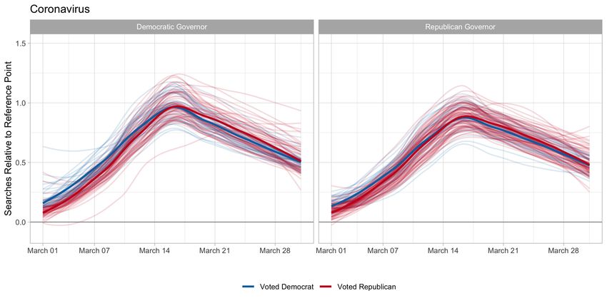
1   Background

    The outbreak of COVID-19 in the USA has prompted unprecedented efforts to prevent disease
spread. In the absence of a vaccine, effective treatments, or widespread testing, individuals’ preven-
tive measures—from hand-washing to physical distancing—are essential for reducing the speed and
extent of the virus’s spread (1). Some measures, such as staying home, are particularly subject to non-
compliance, with possible dire consequences for attempts to “flatten the curve” of new infections.
    Political leaders play an important role in persuading the public to voluntarily comply with costly
preventive measures during pandemics. In addition to issuing orders that serve to reduce contact
between individuals, politicians’ communications about the severity with which individuals should
treat COVID-19 and the preventive measures they should take are likely to be particularly influential
when there is limited information about a novel disease. A better understanding of the link between
politicians’ communications and individuals’ voluntarily adoption of preventive measures is crucial
for ongoing efforts to limit the spread of COVID-19 and for improving public health more generally.
    This study is motivated by three stylized facts that have emerged since the COVID-19 outbreak in
the US. First, both risk perceptions (2; 3; 4) and engagement in preventive behaviors (3; 5) have dif-
fered substantially by individuals’ political party affiliation, with Republicans generally being slower
or less likely to adopt preventive behaviors than Democrats. Second, there have been partisan differ-
ences in the COVID-19 response at the state level, with Democratic governors leading, on average,
more aggressive responses than Republican governors (6). Third, there has been notable within-
party variation in governors’ responses, with some Republican governors taking decisive steps early
on (e.g., in Ohio and Maryland) and other Republican governors being more ambivalent in their
message or reluctant to issue stay-at-home orders. Based on these facts, this Research Note examines
how US governors’ communications influenced individuals’ mobility patterns and engagement in
physical distancing.
    Theoretically, we build on past work that connects public opinion and actions to elites’ cues (7).
Here, constituents use both news outlets and social media to gauge the positions of political elites
whom they trust in order to form their opinions based on these signals (8). Elite cues have been
shown to steer uninformed citizens toward effective policy judgment (9; 10), but they can also cause
citizens to reject valid scientific information (11; 12). While elite cues clearly matter in ‘normal times’
and when the stakes to individuals from following cues is relatively small, it is an open question
of whether and how elite cues might matter during a pandemic in which individuals’ actions can
directly impact their own health.

                                                    2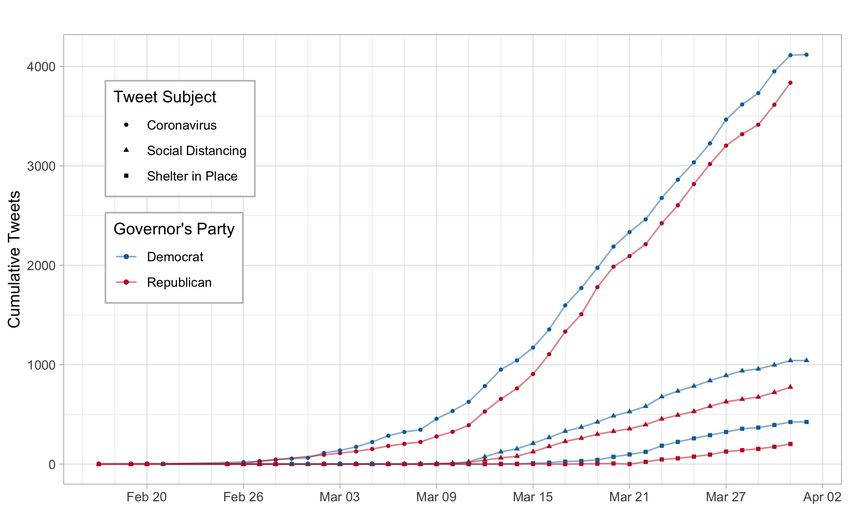
On the one hand, as the US has become increasingly polarized (13), cues from elites who share
citizens’ partisan attachments could have greater effect. On the other hand, research on political
endorsement has shown that elite cues are especially effective when the signal they emit does not
conform with their own party position (14). It is thus possible, for example, that Republican gov-
ernors who communicated the seriousness of COVID-19 in early-March, a period during which the
right-leaning media and US President Donald Trump were skeptical of the risk posted by COVID-19,
would have a stronger effect on Democrats’ behavior than on the behavior of Republicans. Our study
is designed to explore such dynamics.
   Using geocoded county-level data on citizen mobility, past electoral returns that serve as proxy
for partisan preferences, and Twitter-based communications about COVID-19 by governors of all 50
states in the US, this study examines how partisanship mediates the relationship between governors’
COVID-19 communications of governors and residents’ engagement in physical distancing. Specif-
ically, we test the extent to which predominantly Democratic vs. Republican counties respond to
COVID-19 prevention related messaging by their governors. Unlike other recent studies, our focus is
on the effect of governors’ communications encouraging COVID-19 prevention on voluntary behavior
as these often preceded official stay-at-home mandates.
   This paper explores three central questions about the ways in which governors’ messages may
have affected individuals’ engagement in critical COVID-19 prevention behaviors. Rather than focus
on the effect of stay-at-home orders (2; 15), we examine instead the effect of governors’ messages
encouraging physical distancing and limited mobility because these preceded the issuance of orders
by a meaningful number of days or even weeks. We first assess whether governors’ messages affect
individuals’ mobility patterns. Second, we examine whether messages from governors differentially
influence Republican- vs. Democratic-leaning counties. And finally, we assess whether the party
affiliation of governors affects the responsiveness of citizens with differing partisan preferences.
   We find that governors’ messages—as proxied by their Twitter feed—preceded the issuance of
‘stay home’ orders by a meaningful period and had a significant effect on residents’ mobility. These
effects were comparable in magnitude to the effects of ‘stay home’ orders. Second, governors’ com-
munications had, on average, a larger effect on mobility in Democratic counties. Finally, while both
Democratic and Republican counties are equally responsive to Democratic governors, Democratic
counties were more responsive to Republican governors than Republican counties. These results are
consistent with the idea that elites cues that are not aligned with party lines serve as a strong signal
for other-party voters but have more muted effects among own-party voters. Our study contributes
to a better understanding of the nexus of elite cues and citizens’ (voluntary) behavior.

                                                   3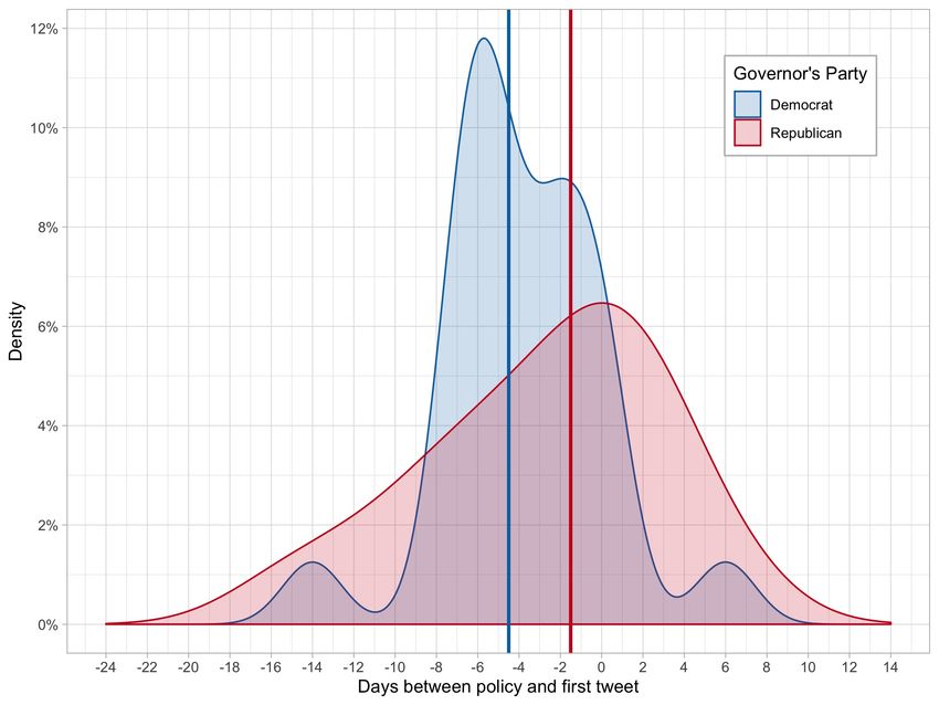
2     Methods and Data

We use the following data to answer the study’s research questions:
     Mobility (physical distancing): Mobility of individuals in US counties is our main outcome of in-
terest. We use publicly released mobility statistics from Safegraph, derived from geolocated devices.1
The Safegraph data comprises a sample of 545 million unique device-days covering 3,140 US counties,
measured continuously throughout the day and reported daily over the period of March 1-March
31, 2020. Using these data, our primary outcome was calculated at the county-day level and defined
as the median time devices from a county spent at home on each day. Using the same data we also
defined secondary outcomes as the share of devices in each county-day pair that stayed at home for
the entire day and the number of miles travelled from home released by Descartes Labs.2 Percent-
age of devices that remained at home during the entire day is a better proxy for physical distancing
than distance travelled, particularly in sparsely populated areas where long-travel distances do not
indicate a lack of physical distancing.
     Risk perceptions: To assess risk perception of individuals, we used data from Google Trends on
searches for the following terms: “Coronavirus,” “social distancing,” “stay at home,” and “shelter in
place.” The higher the search share in a particular location and time period, the higher the perceived
risk among that population (2). Here, we take the daily relative search interest for 202 metro areas for
the period March 1 - March 31 2020. This provides a daily time series for each individual metro area,
yielding 6,262 metro-days. We use these data to show within-metro trends in search interest overtime.
However, these data are not appropriate for cross-sectional comparisons. For cross-sectional compar-
isons, we follow Stephens-Davidowitz and normalize search interest for each of the 202 metro-areas
relative to the metro-day with the greatest search interest over the period of study (16).
     Twitter data: Our main interest lies in explaining health behavior as a function of governors’
messaging (cues) about the necessity of staying home and physical distancing more generally. To
measure such cues, we download all tweets sent from both the personal and official Twitter accounts
of the governors of all 50 US states between February 15th and March 31, 2020.3 We then manually
code each tweet using three binary indicators: (a) whether the tweet is relevant to Coronavirus, and
if so, (b) whether the tweet encourages physical distancing and (c) whether the tweet encourages
staying home (“sheltering-in-place”). Stay home messages necessarily entail physical distancing but
    1 https://www.safegraph.com/dashboard/covid19-commerce-patterns
    2 https://github.com/descarteslabs/DL-COVID-19
   3 For most governors, these tweets are duplicated on their personal and official Facebook page, and the information

the tweets conveyed was repeated in press conferences they held. We thus view governors’ tweets as a proxy for their
messaging efforts more broadly.

                                                          4
not vice-versa (See SI, Section A for additional details). Our key input variable is Post stay-home tweet;
an indicator that has a value of one for all days after the first time a governor explicitly encouraged
staying home. We also check for robustness to using Cumulative stay home tweets, which is the number
of cumulative tweets encouraging staying at home at any given day. Figure 1 shows that, in general,
Democratic governors began encouraging social distancing at earlier date. For example, by March
21, sixteen Democratic governors, but only four Republican governors, have used social media to
encourage state residents to stay home (bottom panel). Figure SI-1 shows that while the median
democratic governor began encouraging staying home 6-7 days before the statutory order, the me-
dian GOP governor began encouraging staying home only a day before the policy came into effect.
Figure SI-2 shows that not merely timing, but also the intensity of Democratic governors’ messaging
about COVID-19 was higher than their Republican counterpart.
Moderators: We test whether the effect of governors’ cues on mobility is moderated by the parti-
san affiliation of governors and counties. GOP governor is an indicator that has the value of one for
Republican governors and zero for Democratic governors. In our main analysis, we measure coun-
ties’ partisanship using Trump vote margin (in units of 10%) in the 2016 presidential elections. In
some analysis, we split the sample by a county’s partisan affiliation. Here, Republican counties are
those in which Trump’s vote margin is larger than zero. We obtain county and state-level electoral
data from the CQ Press Voting and Elections Collection.4
Controls: We control for the number of daily county-level coronavirus positive cases and state-
level deaths using data from the New York Times5 and USAFacts,6 a non-profit civic data clear-
inghouse, and for official physical distancing policies at the state level from Adolph et al. (2020).7
Additional (fixed county-level) control variables are derived from the 5-year American Community
Survey (2014-2018). These include: median household income, median age, population size, educa-
tional attainment by age category, population share over age 65, and the county’s racial composition.
Since the state of Alaska does not report electoral returns at the county-level, we omitted obser-
vations from this state. The analysis sample therefore consisted of 3,100 counties from 49 states and
yielded 94,690 county-day observations. Table 1 report the summary statistics of all variables used in
the empirical analysis.
4 https://library.cqpress.com/elections/
5 https://github.com/nytimes/covid-19-data
6 https://usafacts.org/issues/coronavirus/
7 https://github.com/COVID19StatePolicy/SocialDistancing
5Figure 1: Governors’ tweets by topic
Note: Figure shows the cumulative number of governors tweeting about Coronavirus (top panel), Social
distancing (middle panel), and staying home (bottom panel) by date and governor partisan affiliation. The
governors of Alaska (R), Florida (R), Georgia (R), Iowa (R), South Carolina (R), South Dakota (R) did not
tweet about staying home (shelter-in-place) during this time period.
6Table 1: Summary statistics
Variable Dem counties Republican counties All counties
Outcomes
Median time at home (minutes) 638.41 641.14 640.72
(229.07) (185.42) (192.86)
Log median time at home 6.34 6.38 6.37
(0.64) (0.54) (0.56)
Share of devices home all day 28.40 25.52 25.97
(9.21) (7.91) (8.19)
Log distance traveled 8.87 9.04 9.01
(0.54) (0.61) (0.60)
Independent variables
Tweets about COVID-19 5.05 5.20 5.17
(6.86) (7.85) (7.68)
Tweets about social distancing 1.16 1.15 1.15
(2.27) (2.52) (2.48)
Tweets about staying home 0.45 0.39 0.40
(1.38) (1.42) (1.42)
Post social distancing tweet 0.62 0.61 0.61
(0.49) (0.49) (0.49)
Post stay home tweet 0.30 0.28 0.28
(0.46) (0.45) (0.45)
Trump vote margin -0.19 0.43 0.32
(0.19) (0.19) (0.30)
Covariates
Post-emergency order 0.70 0.68 0.68
(0.46) (0.47) (0.47)
Post-large gatherings ban 0.47 0.41 0.42
(0.50) (0.49) (0.49)
Post-school closure 0.49 0.44 0.45
(0.50) (0.50) (0.50)
Post-restaurant closure 0.44 0.40 0.41
(0.50) (0.49) (0.49)
Post-non-essential business closure 0.17 0.13 0.14
(0.37) (0.34) (0.34)
Post-stay home order 0.19 0.16 0.16
(0.40) (0.36) (0.37)
Confirmed COVID-19 cases 49.48 2.48 11.08
(405.59) (51.52) (180.58)
Median age 38.61 41.90 41.30
(5.28) (5.09) (5.28)
Log household income 10.87 10.80 10.82
(0.35) (0.22) (0.25)
Log population 11.47 10.05 10.31
(1.73) (1.25) (1.46)
Share over 65 0.16 0.19 0.18
(0.04) (0.04) (0.04)
Share black 0.21 0.07 0.09
(0.23) (0.10) (0.15)
Share hispanic 0.15 0.08 0.09
(0.20) (0.11) (0.14)
Share male 0.49 0.50 0.50
(0.02) (0.02) (0.02)
Observations 14708 79982 94690
Counties 484 2616 3100
Table displays means and standard deviations of key variables of interest, as well as the number
of observations and the number of cluster. Sample is 94,690 county-days from March 1-March 31
2020 for which all data are non-missing. GOP counties are those in which Donald Trump’s margin
of victory in the 2016 presidential election was greater than 5%. Democratic counties are all others.
7Estimation Strategy
We use difference-in-differences regressions to estimate the effect of governors’ messaging (as
captured by tweets’ content) on mobility. Our main estimation uses an event study design (be-
fore/after): focusing on the first tweet in which a governor encourages her state residents to stay
home. Our identification assumption is that given parallel trends, once we flexibly control for a
county’s fixed characteristics, and account for both date and county fixed effects, the daily number
of deaths and confirmed COVID-19 cases, the type of state-wide orders issued at any given day,
changes to the number of minutes at home from before to after a governor’s message has a causal
interpretation. See SI Section B for additional details.
3 Results
We present the study’s main results in Table 2. We find that governors’ messages encouraging
residents to stay at home had a positive and significant effect on time spent at home, above and
beyond the effect of state orders encouraging residents to stay home. Averaging across all US counties
(Table 2, Panel A, column 1), a tweet encouraging residents to stay at home increased median time
spent at home by 9.4 minutes per day (or 2.6%) compared to the immediate period before the tweet
was sent. The finding is robust to using minutes at home in levels or in logs, to using alternative
mobility measures (Table SI-4), to using cumulative number of tweets rather than the first tweet
(Table SI-2), and to looking at tweets encouraging physical distancing (Table SI-6).
The effect of governors’ messages on residents’ mobility change were comparable to the effects of
stay-at-home orders (Table 3 and SI Table SI-2). Among all residents, the effects of the tweets were
generally larger than the effects of orders, although the difference between the two effects was not
statistically significant.
We also find suggestive evidence that the effect of governors’ messages encouraging residents to
stay at home were more effective in Democratic-leaning counties than Republican-leaning counties
(Table 2, Panel A, column 2). While the moderating effect of the vote margin for President Trump in
the 2016 general election fell slightly below conventional significance level, the estimates indicate that
a 10% increase in Trump’s vote margin reduced the effect of tweets on mobility by 9 percent. Nonethe-
less, the overall effect of governors’ cues on mobility remained significant in both Democratic- and
Republican-leaning counties (Figure SI-8, left panel).
8Table 2: Governors’ tweets, partisanship, and mobility
Panel A: Full sample
Outcome Median time at home Log time at home
Post stay home tweet 9.382** 12.989** 0.026*** 0.023*
(4.009) (4.950) (0.009) (0.012)
Post stay home tweet × Trump vote margin -1.127 0.001
(0.702) (0.002)
Observations 94690 94690 94690 94690
R2 0.984 0.984 0.998 0.998
County FE Yes Yes Yes Yes
Day FE Yes Yes Yes Yes
Demographics × Day FE Yes Yes Yes Yes
Trump margin × Day FE Yes Yes Yes Yes
COVID controls Yes Yes Yes Yes
Orders Yes Yes Yes Yes
Panel B: By county party
Outcome Median time at home Log time at home
County party Dem GOP Dem GOP
Post stay home tweet 14.768 8.935** 0.035 0.025**
(9.280) (3.780) (0.022) (0.009)
Observations 14708 79982 14708 79982
R2 0.985 0.984 0.997 0.998
County FE Yes Yes Yes Yes
Day FE Yes Yes Yes Yes
Demographics × Day FE Yes Yes Yes Yes
Trump margin × Day FE Yes Yes Yes Yes
COVID controls Yes Yes Yes Yes
Orders Yes Yes Yes Yes
Panel C: Triple interactions
Outcome Median time at home Log time at home
Interaction Cont. vote margin Binary Cont. vote margin Binary
Post stay home tweet 7.421 4.222 0.004 -0.011
(4.732) (7.006) (0.014) (0.027)
Post stay home tweet × GOP governor 12.084 26.960** 0.051** 0.102***
(7.626) (12.779) (0.019) (0.033)
Post stay home tweet × Trump vote margin 0.787 0.006
(1.308) (0.004)
Post stay home tweet × GOP governor × Trump vote margin -3.920** -0.012**
(1.540) (0.005)
Post stay home tweet × GOP county 5.700 0.034
(6.738) (0.027)
Post stay home tweet × GOP governor × GOP county -35.127*** -0.115***
(11.839) (0.034)
GOP county × Day FE No Yes No Yes
Trump margin × Day FE Yes No Yes No
GOP gov × Day FE Yes Yes Yes Yes
GOP county × GOP gov × Day FE No Yes No Yes
Trump margin × GOP gov × Day FE Yes No Yes No
COVID controls Yes Yes Yes Yes
Orders Yes Yes Yes Yes
Observations 94690 94690 94690 94690
R2 0.984 0.984 0.998 0.997
Standard errors in parentheses clustered at the state level. Sample is 96,690 county-days over the period March 1-March 31 2020. Treatment
indicator equals one for all days after the governor of state s issues a tweet encouraging citizens to stay home. “Trump vote margin” is county
i’s vote margin for President Trump in the 2016 election. GOP counties are those in which the Republican vote margin in the 2016 presidential
election was greater than zero. County-level demographic controls are median age, log family income, log population, share of population
over 65, share black, share Hispanic, and share male. COVID controls includes controls for county-level COVID cases and state-level COVID
deaths. “Orders” includes controls for whether the state has issued the following types of orders: emergency declarations, banning large
gatherings, school closures, restaurant/bar closures, non-essential business closures, and stay-at-home orders.
*** p < 0.01, ** p < 0.05, * p < 0.1.
9Table 3: Governors’ tweets and stay at home orders
Outcome Median time at home Log time at home
County party All Dem GOP All Dem GOP
(1) (2) (3) (4) (5) (6)
Post stay home tweet 9.382** 14.768 8.935** 0.026*** 0.035 0.025**
(4.009) (9.280) (3.780) (0.009) (0.022) (0.009)
Post-stay home order 7.895 4.623 8.722* 0.004 -0.011 0.008
(5.215) (10.148) (4.995) (0.012) (0.023) (0.012)
β1 − β2 1.487 10.144 0.213 0.022 0.046 0.017
(6.054) (16.127) (5.521) (0.014) (0.031) (0.014)
Observations 94690 14708 79982 94690 14708 79982
R2 0.984 0.985 0.984 0.998 0.997 0.998
County FE Yes Yes Yes Yes Yes Yes
Day FE Yes Yes Yes Yes Yes Yes
Demographics × Day FE Yes Yes Yes Yes Yes Yes
Trump margin × Day FE Yes Yes Yes Yes Yes Yes
COVID controls Yes Yes Yes Yes Yes Yes
Sample is 94,690 county-days between March 1 and March 31, 2020. Treatment indicator
equals one for all days after the governor of state s issues a tweet about staying home. “Trump
vote margin” is county i’s vote margin for Donald Trump in the 2016 presidential election.
GOP counties are those in which the Republican vote margin in the 2016 presidential elec-
tion was greater than zero. County-level demographic controls are median age, log fam-
ily income, log population, share of population over 65, share black, share Hispanic, and
share male. COVID controls account for county-level COVID confirmed cases and state-level
COVID deaths. “Orders” includes indicators for whether the state has issued the following or-
ders: emergency declaration, banning large gatherings, school closures, restaurants closures,
non-essential business closures, and stay-at-home orders. Standard errors clustered at the
β
state level. β12 is the ratio of tweet to stay at home coefficients.
*** p < 0.01, ** p < 0.05, * p < 0.1.
10Panel B of Table 2 shows that the effect of governors’ first stay-at-home tweet on mobility was
1.6 times larger in counties that voted for Hilary Clinton (15 minutes, or 3.5 percent) than in counties
that voted for President Trump (9 minutes, or 2.5 percent). This finding was further reinforced in the
event-study plot of the estimated daily mobility change before and after the first tweet encouraging
residents to stay at home (Figure 2). While there was always a discernible effect on mobility within
2-3 days after the first message from a governor, the effect was substantively more pronounced in
Democratic-leaning counties (left panel).
Figure 2: Event study: governor tweets “stay home,” by subsamples
100 100
Median time at home (minutes)
Median time at home (minutes)
50 50
0 0
-50 -50
-10 -5 0 5 10 15 -10 -5 0 5 10 15
Day relative to tweet Day relative to tweet
Democratic county Republican county
Note: Figure shows coefficients from a county-level event-study regression of median time at
home on indicators for leads and lags of the treatment (an indicator equaling 1 for all days after
a governor issues her first tweet encouraging citizens to stay at home). Models include county
and date fixed effects. Sample is split by Democratic counties (left panel) and Republican counties
(right panel).
In models that tested whether county residents’ partisan preference and governors’ party affilia-
tion moderated the effect of governors’ messaging on mobility patterns (Table 2, Panel C), we found
that Republican governors in particular have differing effects on Democratic- vs. Republican-leaning
areas. To ease the interpretation of the triple-interaction models in Panel C, we divided the sample
by governors’ party affiliation and estimated the effect of governors’ tweets on mobility conditional
on President Trump’s vote margin (SI Table SI-3).
In states with a Democratic governor, there was no significant difference between the responses
of Democratic and Republican voters: the interaction of tweet and President Trump’s vote margin
is not significant (SI Table SI-3, Panel A, column 2). However, in states with a Republican governor,
Democratic-leaning counties responded more strongly than Republican-leaning counties. In such
states, a higher vote margin for President Trump was significantly associated with a smaller effect of
communications on mobility (SI Table SI-3, Panel B, column 2).
11These dynamics are further explored in Figure 3, which plots the marginal effect of the first tweet
by a governor on mobility reported in SI Table SI-3. Panel A shows that the response to tweets
from Republican governors encouraging residents to stay at home was strongly decreasing in Pres-
ident Trump’s vote margin, while under Democratic governors (Panel B), it was weakly (but not
significantly) increasing. The most responsive counties are Democratic-leaning areas in Republican
states, while the least-responsive are deeply conservative areas in Republican states.8 Since the lat-
ter comprise most of the data in Republican states, this leads to a smaller effect size (7.92 minutes
increase post-tweet) in Republican states when averaging across the political spectrum (Table SI-3,
Panel B, column 1). In contrast, both Democratic- and Republican-leaning counties in Democratic
states respond similarly to their governor’s messaging, yielding a somewhat larger average effect of
10 minutes (Table SI-3, Panel A, column 1).
Finally, with the exception of deeply conservative areas whose response diverges under different
governors, Republican-leaning counties in general respond similarly to messaging from Republican
and Democratic governors. For example, in states with a Democratic governor, the median county
with respect to President Trump vote margin is Trump +29.5%. Using the coefficients of SI Table SI-3,
Panel A, column 2 the first ‘stay home’ tweet increase time at home by 10.84 minutes.9 Similarly,
in states led by a Republican governor, the effects of governor’s tweet in a Trump +29.5% county is
estimated to be 11.28 minutes.10
4 Discussion
Governments play a central role in combating pandemics by financial the development and test-
ing of vaccines and treatments, scaling-up testing and contact tracing, and coordinating the response
of various agencies and institutions. Yet the success of efforts to prevent the spread of infectious
diseases depends crucially on the actions taken by individuals who are asked to voluntarily comply
with costly measures to prevent transmission. This study shows the importance of state governors’
messaging efforts, but also that political party preferences influenced individuals’ responses to com-
munications from governors about the need to engage in social distancing and stay at home during
the outbreak of the novel coronavirus in the US. We report three key findings.
8 In
Republican states, in the median Democratic county (Trump -22%), Democrats responded to a ‘stay home’ tweet by
their GOP governor by increasing time at home by 29.8 minutes. By contrast, in those states, governors’ messages were
associated with 6 minutes increase in time spent at home in the median Republican county (here, President Trump’s vote
margin is +45%).
9 The estimate is 6.197 + 1.576 × 2.95 = 10.84.
10 The estimate is 21.233 − (3.373 × 2.95) = 11.28 using the coefficients of SI Table SI-3, Panel B, column 2.
12Figure 3: Predictive margins: effect of “stay home” tweet by Trump vote share and governor party
(a) Republican governors (b) Democratic governors
Marginal Effect of stay home tweet on time at home
Marginal Effect of stay home tweet on time at home
60
60
40
40
20
20
0
0
-20 -20
-40 -40
-1 -.5 0 .5 1 -1 -.5 0 .5 1
Moderator: Trump margin Moderator: Trump margin
Note: Figure shows predicted values and 95% confidence intervals from a county-level regression
of median time at home on the treatment indicator, its interaction with Donald Trump’s county-
level vote share in the 2016 presidential election, county and day fixed effects, as well as day
fixed effects interacted with control variables and Trump’s 2016 margin, see Table SI-3 Panels
A and B. The treatment is an indicator variable equaling 1 for all days after a governor issues
their first tweet encouraging citizens to stay at home. We estimate the model separately for states
with Democratic (Panel A) and Republican (Panel B) governors. The fitted line shows the linear
marginal effect of the treatment at different levels of Trump vote share for each state type. The
points with 95% confidence intervals show semi-parametric estimates of the marginal effect of the
treatment at five different bins of Trump vote share. Bins are (-1,-0.25), (0.25, 0), (0, 0.25), and (0.25,
0.5). The histogram below the predicted margins displays the density of the county-level Trump
vote margin by treatment status (red is treated, grey is untreated).
13First, Democratic and Republican governors’ messaging on COVID-19, which preceded the day
in which stay-at-home orders were issued, was associated with a significant reduction in mobility in
both Democratic-leaning and Republican-leaning counties.11 This finding is consistent with the idea
that political leaders can strongly influence the behavior of their constituents and achieve higher
compliance with prevention measures during a public health crisis. Importantly, governors’ messag-
ing affected the behavior of citizens with congruent preferences (i.e., same party as the governor), but
also of citizens with incongruent preferences. One reason governors’ messaging can be consequen-
tial is by explaining why individuals are asked to take costly actions. Google Trends searches, which
are an indicator of interest in an issue (2; 16)), show that governors’ cues increased the frequency of
search terms related to social distancing and staying home and these increases occurred days before
stay-at-home orders were issued (Table SI-1).
Second, Republican-leaning counties responded less strongly than Democratic-leaning counties
to messages from governors encouraging residents to stay at home. This finding persisted even after
controlling for state fixed effects and county-level socio-economic characteristics, and it is consistent
with a growing literature that finds both differential levels of social distancing by partisan affilia-
tion (4), as well as differential responses to stay-at-home orders (3; 2; 15).
Third, and most notably, Democratic counties were especially responsive to cues from Republi-
can governors. The reduction in mobility induced by a Republic governor was estimated to be about
25 minutes in counties where President Trump lost by 10% in the 2016 general election (Table SI-3,
Panels B). In contrast, the effect of Democratic governors on mobility in similarly Democratic-leaning
counties was 5 times lower, with only a 5 minute reduction in mobility (Table SI-3, Panels A). This
finding is consistent with the literature on partisanship and the effects of political leaders’ endorse-
ments. Republican governors who sounded the alarm on COVID-19 sent a strong and consequential
signal to citizens aligned with the opposite political party since those governors’ messages were in
contrast to the general views held by Republican leaders about COVID-19. In short, elite cues were
stronger when they did not conform with the party affiliation of the elites. Republican governors
who broke with national party members sent a strong signal to their Democratic constituents. How-
ever, Democratic governors were largely expected to encourage social distancing, blunting the force
of the signal and therefore the overall effects of their messages.
Indeed, the fact the GOP leaders were sending mixed messages about COVID-19 helps explain
why the effect of Republican governors’ messaging on mobility was stronger in Democratic coun-
11 We note that when weighting by population (Figure SI-8), the effect of governors’ messaging on mobility is no different
than zero in deeply conservative Republican counties where Trump’s vote margin is over 40%.
14ties and moderate Republic counties than conservative strongholds. This result is consistent with a
“backlash” effect, whereby conservative Republican areas react to signals from their local Republican
leaders that contradict national-level party messaging with either indifference or outright hostility.
Under Democratic governors, this backlash effect is absent as Democratic governors’ calls for isola-
tion did not conflict with national-level party messaging.
This study has several limitations. Messages from governors’ encouraging social distancing and
staying at home were obtained from their Twitter accounts, which may not have been the primary
mode of communication to constituents. However, these messages were likely to be closely accom-
panied with other forms of communication to constituents, such as radio and television. Another
limitation is the Twitter messages encouraging residents to stay at home may have been correlated
with the voluntary closure of workplaces, which may have been the reason why individuals tended
to spend more time at home. While this can affect the magnitude of the association between mes-
sages and mobility, our analyses do control for the issuance of various orders for schools and other
institutions to close. Moreover this should not have as strong an effect the associations found with
political preferences of county residents.
This study demonstrates how and why political partisanship has influenced citizens’ decisions to
voluntarily engage in social distancing and reduce their mobility in response to communications by
their state governor during the COVID-19 outbreak in the US. The results support several theories
of how elite cues influence public opinion and actions, and they provide valuable insights on how
governors’ communications can influence behavior in the ongoing response to COVID-19.
ACKNOWLEDGEMENT
We wish to thank Balyey Tuch, Emma Carlson, Caroline Riise and Michael Nevett for excellent
research assistance, and Penn’s Development Research Initiative (PDRI) for logistical support.
15References
[1] M. U. Kraemer, et al., Science (2020).
[2] J. M. Barrios, Y. V. Hochberg, Risk perception through the lens of politics in the time of the
covid-19 pandemic (2020). University of Chicago, Becker Friedman Institute for Economics.
[3] H. Allcott, et al., Polarization and public health: Partisan differences in social distancing during
covid-19 (2020). NBER Working Paper No. 26946.
[4] S. Kushner Gadarian, S. W. Goodman, T. B. Pepinsky, Health Behavior, and Policy Attitudes in the
Early Stages of the COVID-19 Pandemic (March 27, 2020) (2020).
[5] S. Engle, J. Stromme, A. Zhou, Staying at Home: Mobility Effects of COVID-19 (2020). Working
paper.
[6] C. Adolph, K. Amano, B. Bang-Jensen, N. Fullman, J. Wilkerson, medRxiv (2020).
[7] J. R. Zaller, et al., The Nature and Origins of Mass Opinion (Cambridge university press, 1992).
[8] G. S. Lenz, Follow the leader?: how voters respond to politicians’ policies and performance (University
of Chicago Press, 2013).
[9] S. L. Popkin, The Reasoning Voter: Communication and Persuasion in Presidential Campaign (Univer-
sity of Chicago Press, 1994).
[10] A. Lupia, M. D. McCubbins, L. Arthur, et al., The democratic dilemma: Can citizens learn what they
need to know? (Cambridge University Press, 1998).
[11] D. Darmofal, Political Research Quarterly 58, 381 (2005).
[12] R. J. Brulle, J. Carmichael, J. C. Jenkins, Climatic change 114, 169 (2012).
[13] S. Iyengar, Y. Lelkes, M. Levendusky, N. Malhotra, S. J. Westwood, Annual Review of Political
Science 22, 129 (2019).
[14] C.-F. Chiang, B. Knight, The Review of Economic Studies 78, 795 (2011).
[15] M. O. Painter, T. Qiu, Political beliefs affect compliance with covid-19 social distancing orders
(2020). Working paper.
[16] S. Stephens-Davidowitz, A. Pabon, Everybody lies: Big data, new data, and what the internet can tell
us about who we really are (HarperCollins New York, 2017).
16SUPPLEMENTARY INFORMATION
— For Online Publication —
A Twitter data
We use governors’ tweets to capture their public messages (cues). In this section we describe how
this measure was devised. First, we identified both the official and the personal Twitter accounts of
all USA governors. We then collected tweets published by these accounts between February 15th
and March 31st . For this purpose, we wrote a simple script to download tweets via Twitter API
(Application Programming Interface) using R (version 3.5.1). We removed quoted tweets (tweets
directly citing other tweets) and retweets from the downloaded dataset. Replying tweets (tweets
directly replying to other tweets) were also excluded, except for the cases where a replying tweet and
an original one were written by the same account (threads).
We downloaded a total of 11,266 tweets from the official and personal accounts of the governors
of 50 USA states and the President. The tweets were aggregated into a single CSV file, and then coded
using research assistants that were trained based on the following codebook:
A.1 Instructions to code governors’ Twitter feed
For each tweet, we follow the following steps:
1. Identify if the tweet is about the COVID-19/Coronavirus crisis. If yes, mark 1 in the column
titled “covid related.” If no, mark 0 and move to the next tweet.
2. If yes, then identify whether the tweet is related to social distancing. If it is, mark 1 in the
social distance column. If not, mark 0.
3. Then identify whether the tweet is related to shelter in place. If it is, mark 1 in the shel-
ter in place column. If not, mark 0.
1. Coronavirus related: This includes all tweets that relate to the current COVID-19 crisis, whether
or not they explicitly mention the words “coronavirus” or “Covid-19.” For example, consider the
following tweet. While it does not explicitly mention the name of the virus, it clearly refers to the
coronavirus crisis.
“Have supplies on hand, but don’t hoard. Contact your healthcare provider about obtaining extra
necessary medications to have on hand.”
SI-12. Social distancing: This includes all tweets that encourage, explain, or otherwise refer to the con-
cepts of social distancing. Some key words and phrases to look out for in these tweets will be “avoid
gatherings / crowded places / large events,” “physical distancing,” “keep 6 feet apart,” and “flatten
the curve”. These key words are simply examples; they are NOT exhaustive. Please note that calls to
“avoid sick people/people with symptoms” are NOT calls to social distancing. There is a distinction
between tweets about avoiding your own infection (e.g., wash your hands, avoid sick people, etc),
and those that focus more on not spreading the disease as a transmission vector. We care about the
latter. For example:
“There are steps every Arizonan can take to prevent the spread: Wash your hands for at least 20
seconds; Avoid touching your eyes, nose and mouth; Avoid close contact with people who are sick;
Cover your cough or sneeze.
Is not about social distancing, since it only mentions how to prevent your own infection. In contrast,
the tweet below is about social distancing, because it mentions “stay away from crowds”
“Don’t fear covid19 virus, just be smart. Wash your hands. Don’t shake hands, stay home if not
feeling well, stay away from crowds. These simple steps will keep most of us away from the
hospitals. It isn’t the end of the world. Just focus on good hygiene and change a few habits.”
3. Shelter in place: This refers to tweets that explicitly call on citizens to stay at home and avoid
going out for non-essential business. Some key words to look out for are “stay home,” “work from
home” “shelter in place,” “safer at home.” These key words are simply examples; they are NOT
exhaustive. For example, the tweet below explicitly calls on people to stay home and should be
coded as 1. However, the tweet below it does not call for staying at home, just social distancing.
“Reminder to our young people: you are not immune to #COVID19 or invincible. You can get
coronavirus and you can spread it to loved ones. Don’t be selfish. Take this seriously. Stay safe,
stay home.”
“Social distancing is a primary protective measure to flatten the curve of this virus. I cannot un-
derscore the seriousness of following these measures to help our neighbors, friends, and families.”
Finally, note that staying home is a form of extreme social distancing. Therefore all stay home tweets
should also be social distancing tweets. However, the reverse is not true. There may be weaker forms
of social distancing that are not fully stay home.
SI-2B Estimation strategy
To estimate the baseline effect of messaging, we estimate a simple differences-in-differences re-
gression using a two-way fixed effects specification for county i in state s day t
0
yist = α + θTWEETst + δt + ξ i + Xist β + eist
Where TWEETst is a treatment indicator that equals one in all periods after the governor of state s
issues a tweet encouraging citizens to stay home and δt are day fixed effects and ξ i are county fixed
effects. Xist is a vector of county and state-level control variables, which are either time-varying or, if
fixed, then interacted with day fixed effects δt . Controls are current and lagged confirmed COVID-19
cases, county-level demographics including median age, log family income, log population, share
over 65, share black, Hispanic, white, and male, as measured in the most recent American Com-
munity Survey (ACS), and dummies for state-days in which various stay home orders are in effect.
We include the following state-level orders: emergency declaration, banning large gatherings, school
closures, closures of non-essential businesses, closure of bars/restaurants, and stay home/shelter in
place orders.
We consider several different specifications, including measuring the independent variable TWEETst
as the cumulative number of “stay home” tweets issued in the past 3 or 5 days, or one-day lagged
number of stay home tweets. We also consider similar specifications where the tweets of interest are
those encouraging social distancing. For these regressions, we cluster our standard errors at the level
of the state, since all counties within a state are perfectly correlated in their treatment exposure. We
estimate this difference-in-differences regression on the entire sample, and on GOP and Democratic
counties separately.
To estimate the dynamic effects of messaging, as well as test pre-trends in the outcome variable
before a tweet was issued, we estimate the following event-study regression using a two-way fixed
effects specification for county i in state s day t
15
yist = α + ∑ 0
θτ TWEETsτ + δt + ξ i + Xist β + eist
τ =−10
Where τ indicates leads and lags of the treatment period, TWEETsτ are dummies for these leads and
lags, and θτ , τ > 0 give the dynamic treatment effects while θτ , τ < 0 test pre-treatment trends. The
omitted reference period is τ = −1. We estimate this event-study regression on the entire sample,
and on GOP and Democratic counties separately.
SI-3To estimate the effect of messaging by county-level political affiliation, we estimate several triple-
difference models using two-way fixed effects for county i in state s day t. In the first set of these
models, we interact the exposure to state-level messaging with county-level variation in political
affiliation.
0
yist = α + ϕ1 TWEETst + ϕ2 TWEETst × MARGI Ni + δt + δt × MARGI Ni + Xist β + ξ i + eist
In this case, MARGI Ni is county i’s Republican vote share – measured as Donald Trump’s 2016
margin of victory. In these specifications, we also cluster standard errors conservatively at the county
level, even though the variation of interest –the interaction term – is at the county-year level.
Finally, to test whether the county-level partisans response to political messaging varies by the
governor’s party, we consider the quadruple-difference estimation strategy:
yist = α + φ1 TWEETst + φ2 TWEETst × MARGI Ni + φ3 TWEETst × GOPGOVs
+ φ4 TWEETst × GOPGOVs × MARGI Ni + δt + δt × MARGI Ni
0
+ δt × GOPGOVs + δt × GOPGOVs × MARGI Ni + ξ i + Xist β + eist
We consider specifications where MARGI Ni is measured as a continuous measure of Trump’s
2016 vote margin, or an indicator variable equaling one if Trump won the county in 2016. In the
binary case, φ1 gives the effect of the governor’s tweet in Democratic states in centrist counties, φ1 +
φ2 is the effect in Trump-supporting counties of Democratic states, φ1 + φ3 is Democratic counties
under Republican governors, and φ1 + φ2 + φ3 + φ4 the effect of the tweet in the Republican counties
of Republican states. The quadruple-difference model is completed by the relevant two- and three-
way interactions with the day fixed effects.
SI-4C Supplementary figures
C.1 Descriptive information on Governors’ tweets
In this section, we present basic descriptive information on the dataset of governors’ tweets de-
scribed in Appendix A.
In Figure SI-1, we calculate the state-level difference between the date of the first stay-at-home
order and the date of the first tweet encouraging citizens to stay home/shelter-in-place. Negative
numbers indicate that the tweet was issued before the policy, and positive numbers indicate the
opposite. We then plot the distribution of these differences separately for Republican and Democratic
governors, with vertical lines to indicate the group-specific median number of days between order
and tweet. While the earliest tweeters appear to be Republican governors, the peak of the Democratic
distribution is well to the left of zero, with a median of -6. In contrast, the Republican distribution
is clustered near zero, with a median of -1.5. On average, Democratic governors tweet about staying
home far before implementing orders, while Republican governors typically only tweet about staying
home in the days leading up to and after an order is issued.
In Figure SI-2, we plot the cumulative number of tweets over time, separately by tweet subject and
governor party. Comparing across tweet subjects, we find that governors tweet substantially more
about COVID-19/coronavirus in general than they do about specific recommendations for either
social distancing or staying at home. Democratic governors tweet more and earlier about all three
topics.
SI-5Figure SI-1: Days between date of stay at home order and date of first tweet
Note: Figure shows the distribution of the difference in days between the governors’ first tweet explicitly
encouraging sheltering-in-place and the state’s first official stay-at-home order. Vertical lines indicate median
difference in days for each party.
Figure SI-2: Intensity of Governors’ COVID-19 tweets over time
Note: Figure shows the cumulative number of governors’ tweets about a topic, by topic, date, and governor
party. Tweet topic is indicated in legend.
SI-6C.2 Google Trends
In this section, we consider trends in Google search interest for various search terms as a proxy
for citizens’ beliefs about coronavirus-related topics. First, we de-normalize the raw Google trends
data such that all metro-day units are normalized relative to a single reference point. In Figure SI-3
we plot search interest over time for “social distancing” in Panel A and “coronavirus” in Panel B,
for each metro area. We split these plots by metro areas under Democratic governors (left panel) vs.
Republican governors, (right panel) and then overlay the mean search interest trend separately for
metro areas that voted Republican vs. Democratic in the 2016 presidential election. All trends are
estimated with a lowess smoother.
In Panel A, we see that mean search interest in social distancing among voters of both parties
begins earlier and is greater under Democratic governors, likely because, as Figure SI-2 makes clear,
Democratic governors are tweeting about social distancing earlier and more frequently than Republi-
cans. In addition, across states of different parties, mean search interest in social distancing is always
greater in Democratic-leaning metro areas. However, these partisan gaps differ depending on the
identity of the governor. The partisan difference in search interest between voters is greater than
among Democratic than Republican governors. Importantly, we see no such partisan differences –
either across or within states – in search interest for “coronavirus.” Therefore, while all citizens, re-
gardless of political beliefs or governor identity, exhibit equal mean search interest for coronavirus,
there are substantial differences in interest for social distancing. These patterns suggest a potentially
interesting interaction between citizen and governor identity in forming beliefs about the merit of
voluntary social distancing interventions.
SI-7Figure SI-3: Google search interest by partisan alignment and governor’s party over time
(a) Social distancing
(b) Coronavirus
Note: Figure shows the daily relative Google search interest for the term “social distancing” in Panel A and
“Coronavirus” for 205 metro-areas in the United States from March 1-March 31. All search numbers are
normalized relative to a reference group. Trends are adjusted using a lowess smoother. Metro-areas are
defined as “Republican” if Donald Trump’s margin of victory in the 2016 presidential election is greater than
5%. Thick lines indicate mean search interest across metros for republican and democratic states.
SI-8C.3 Mobility before and after stay-at-home orders
In this section, we analyze trends in mobility before and after state-level shelter-in-place/stay-at-
home orders are issued for each of the four mobility outcomes. We estimate trends separately before
and after the issuing of stay-at-home orders using a third-order polynomial. Across each outcome
in Figure SI-4, we find that mobility reduces substantially before the stay-home order was issued.
In fact, reductions in mobility are approximately equal in magnitude before and after the order, and
the slope of the trend function does not meaningfully differ. This indicates that the pre-order period
in which behavior change is broadly voluntary is critical for understanding behavioral responses to
coronavirus.
Figure SI-4: Mobility relative to stay at home orders
(a) Median time at home (b) Log time at home
850
6.7
800
Median time at home (minutes)
6.6
Log median time at home
750
6.5
700
6.4
650
6.3
600
-10 -5 0 5 10 -10 -5 0 5 10
Day relative to lockdown Day relative to lockdown
(c) Share home all day (d) Log distance traveled
40 9.1
9
Share of devices home all day
Log distance traveled
35
8.9
8.8
30
8.7
25 8.6
-10 -5 0 5 10 -10 -5 0 5 10
Day relative to lockdown Day relative to lockdown
Note: Figure shows trends in mobility, as measured by median home dwelling time (Panel A), log of median
home time (Panel B), the share of location-enabled devices home all day (Panel C), and the log of median
distance traveled (Panel D) relative to the governors’ issuance of a statewide stay-home order. Points indicate
means in the outcome variable across counties for a given day relative to the stay-home order, with 95%
confidence intervals. Trends are estimated parametrically with a third-order polynomial separately before
and after the stay-home order.
SI-9C.4 Event study plots
In this section, we assess the plausibility of the key assumption of our empirical strategy – that
counties governed by governors that issued stay-home-related Twitter communications exhibit paral-
lel trends in mobility relative to those in states that do not. To provide evidence for this assumption,
we analyze the pre-treatment trends of the key mobility outcomes in treatment relative to control
counties. We estimate pre-trends using the standard event-study regression model described in Ap-
pendix B, in which the outcome is regressed on dummy variables for leads and lags of the treatment,
as well as controls and fixed effects.12 The event-study model also allows us to estimate the dynamic
path of effects in order to determine the “onset” time of the treatment, as well as whether the effects
fade or grow over time.
Figure SI-5 plots the coefficients from the event-study regression for the four major outcomes –
median home time, log median home time, share of devices home all day, and log distance travelled
– in the full sample. In general, we see that parallel trends appear to hold; across all four outcomes,
only one of the pre-period coefficients out of 40 are significantly different from zero at the 5% level.
In contrast, the post-period coefficients are generally positive and significant, with the effects most
pronounced for median time at home (Panel A) and share home all day (Panel C). In general, a
stay-home tweet does not produce an immediate response, but rather takes 2-3 days to generate
change in behavior. This makes sense if the first tweet marks a change in messaging that is followed
by more tweets on the subject. The coefficients then rise monotonically (or fall, in Panel D) before
plateauing 10-11 days after the initial tweet. For median time home – our main outcome of interest –
the maximum daily impact of a tweet on behavior occurs on day 11 and corresponds to 29.4 minute
increase in daily time at home, on average, or a 4.5% increase, as we can see from Panel B.
Figure SI-6 then splits the sample by county-level partisan alignment to test whether the assump-
tion of parallel trends is likely to hold in these subsamples, as well as to compare the dynamic effect
sizes by party. Again the parallel trends assumption seems likely to be satisfied, as pre-period co-
efficients are clustered around zero and are rarely significant. In general, the effect sizes do appear
larger among the sample of Democratic counties. However, due to a much larger sample, the Re-
publican coefficients are more precisely estimated. This provides at least suggestive evidence that
Democrats respond more actively to their governors’ stay home messaging with voluntary behavior
change, though the differences in the event-study coefficients by party are unlikely to be statistically
significant given the wide confidence intervals in the Democratic sample.
12 Recallthat the treatment date is defined as the date when the governor first issued a tweet encouraging individuals to
stay home.
SI-10You can also read