Populations of planets in multiple star systems
←
→
Page content transcription
If your browser does not render page correctly, please read the page content below
Populations of planets in multiple star systems

                                               David V. Martin
arXiv:1802.08693v1 [astro-ph.EP] 23 Feb 2018

                                               Abstract Astronomers have discovered that both planets and binaries are abundant
                                               throughout the Galaxy. In combination, we know of over 100 planets in binary and
                                               higher-order multi-star systems, in both circumbinary and circumstellar configura-
                                               tions. In this chapter we review these findings and some of their implications for the
                                               formation of both stars and planets. Most of the planets found have been circum-
                                               stellar, where there is seemingly a ruinous influence of the second star if sufficiently
                                               close (. 50 AU). Hosts of hot Jupiters have been a particularly popular target for
                                               binary star studies, showing an enhanced rate of stellar multiplicity for moderately
                                               wide binaries (beyond ∼ 100 AU). This was thought to be a sign of Kozai-Lidov
                                               migration, however recent studies have shown this mechanism to be too inefficient
                                               to account for the majority of hot Jupiters. A couple of dozen circumbinary planets
                                               have been proposed around both main sequence and evolved binaries. Around main
                                               sequence binaries there are preliminary indications that the frequency of gas giants
                                               is as high as those around single stars. There is however a conspicuous absence
                                               of circumbinary planets around the tightest main sequence binaries with periods of
                                               just a few days, suggesting a unique, more disruptive formation history of such close
                                               stellar pairs.

                                               Introduction

                                               It is known that roughly half of Sun-like stars exist in multiples and about a third in
                                               binaries (Heintz 1969; Duquennoy & Mayor 1991; Raghavan et al. 2010; Tokovinin
                                               2014). It is also known that extra-solar planets are highly abundant, with most stars
                                               hosting at least one planet (Howard et al. 2010; Mayor et al. 2011; Petigura et al.
                                               2013). The next step is to connect the two concepts and pose the question of planets

                                               David V. Martin
                                               Fellow of the Swiss National Science Foundation at the University of Chicago
                                               e-mail: davidmartin@uchicago.edu

                                                                                                                                     1
2 David V. Martin
in binaries. Such planets are often thought of as exotic examples of nature’s diver-
sity. However, considering the ubiquity of both planets and binaries throughout the
Galaxy, the question of their coupled existence is in fact natural.
We first cover a few important aspects of stellar multiplicity and the configu-
rations, stability and dynamics of planets in binaries. The rest of this chapter is
devoted to analysing the observed populations of planets in binaries. Some of the
implications for planet formation are also discussed.
Stellar multiplicity
The seminal work of Raghavan et al. (2010) draws upon binary and higher-order
multi-star systems discovered with a variety of techniques. Two of the most im-
portant results are the multiplicity rate of stars and the separation distribution for
binaries. These two results are shown in Fig. 1. For FGK stars that are typically
considered for exoplanet surveys ∼40-50% of stars have additional companions.
The multiplicity is higher for more massive stars and lower for less massive. For
binary stars the distribution of separations can be reasonably fitted by a log-normal
function with a mean of 293 years. In terms of semi-major axis, this corresponds to
roughly 50 AU for a mass sum MA + MB = 1.5M . This distribution of separations
is calculated using primaries of all masses. When split into different primary spec-
tral types, the semi-major axis distribution grows wider as a function of increasing
primary mass.
log (binary semi-major axis) (AU)
-2 -1 0 1 2 3 4 5
100 50
Percentage of stars with companions
80 40
Number of binaries
60 30
40 20
20 10
0 0
O B A F G K M L T -2 0 2 4 6 8 10
Spectral type log (binary period) (days)
Fig. 1: Left: stellar companion percentage as a function of spectral type. Right: pe-
riod distribution of observed binaries, with a semi-major axis distribution calculated
assuming a mass sum of 1.5M , which is the average observed value. The dashed
line is a fitted log-normal distribution with a mean of log Tbin = 5.03 and a standard
deviation of σlog Tbin = 2.28. Both figures are adapted from Raghavan et al. (2010),
with the data taken from sources listed in that paper.Populations of planets in multiple star systems 3
Orbital configurations
There are two types of orbits in which planets have been discovered in binary star
systems. First, the planet may have a wider orbit than the binary (ap > abin ) and
orbit around the barycentre of the inner binary. This is known as a circumbinary or
“p-type” planet. Alternatively, the planet may have a smaller orbit than the binary
(ap < abin ) and only orbit around one component. This is known generally as a
circumstellar or “s-type” planet, or as a circumprimary or circumsecondary planet
as a function of which star is being orbited1 . These configurations are illustrated in
Fig. 2. Other, more exotic orbits in binaries have been considered, such as trojan
planets near L4 and L5 (Dvorak 1986; Schwarz et al. 2015) and halo orbits near L1,
L2 and L3 (Howell 1983). No such planets have been discovered though.
s-type planets p-type planets
circumprimary
planet
primary secondary
star star
primary
star circumbinary
planet
secondary
star
circumsecondary
planet
Fig. 2: Left: circumstellar “s-type” planets in binaries, individually around both pri-
mary and secondary stars. Right: circumbinary “p-type” orbits in binaries collec-
tively around both stars.
Orbital stability
There is a limit to where a planet may have a stable orbit in a binary star system.
This has a profound effect on the observed populations, by carving away unstable
regions of the parameter space. Much of the work to derive three-body stability lim-
its was undertaken even before planets were discovered in binaries (Ziglin 1975;
Black 1982; Dvorak 1986; Eggleton & Kisseleva 1995; Holman & Wiegert 1999;
Mardling & Aarseth 2001; Pilat-Lohinger et al. 2003; Mudryk & Wu 2006; Doolin
& Blundell 2011). The classic method has been to run numerical N-body simula-
1 These terms were first coined in Dvorak (1986) and stand for “planet-type” and “satellite-type”.4 David V. Martin
tions over a parameter space and determine regular and chaotic domains. The often-
quoted work of Holman & Wiegert (1999) used this method to derive empirical
stability limits for both circumbinary and circumstellar planets.
Circumbinary planets have stable orbits beyond acrit ,
acrit
= 1.60 + 5.10ebin − 2.22e2bin + 4.12µbin − 4.27ebin − 5.09µbin
2
+ 4.61e2bin µbin
2
,
abin
(1)
where abin is the semi-major axis of the binary, ebin is the eccentricity of the bi-
nary and µbin = MB /(MA + MB ) is the reduced mass of the binary. This does not
account for eccentric or misaligned planets or resonances, which can create islands
of both stability and instability (Doolin & Blundell 2011). For circumstellar orbits
the widest planet orbit acrit is
acrit
= 0.464 − 3.80µbin − 0.631ebin + 0.586ebin µbin + 0.150e2bin − 0.198µbin e2bin .
abin
(2)
For details, including error bars on the coefficients of Eqs. 1 and 2 see Holman
& Wiegert (1999).
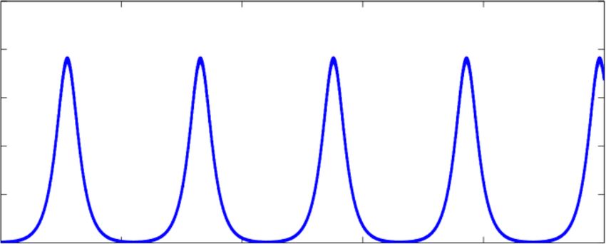
Kozai-Lidov cycles
For circumstellar planets in binaries one must consider the Kozai-Lidov effect,
which is named after the pioneering work of Lidov (1961, 1962); Kozai (1962). If
the planet and binary orbits are misaligned between 39◦ and 141◦ then there is a sec-
ular oscillation of both the planet’s eccentricity, ep , and its inclination with respect
to the binary, Ip . An example is shown in Fig. 3. An initially circular circumstellar
planet obtains a maximum eccentricity of
r
5
ep,max = 1 − cos2 Ip,0 , (3)
3
where Ip,0 corresponds to the planet’s inclination at ep = 0. This is derived to
quadrupole order, under the assumption that the outer orbit (here the binary) car-
ries the vast majority of the angular momentum. The outer eccentricity and incli-
nation do not change. More general equations that can be applied to any inner and
outer angular momenta were derived in Lidov & Ziglin (1976); Naoz et al. (2013);
Liu et al. (2015). For circumbinary planets, where the outer angular momentum is
typically negligible, the Kozai-Lidov effect practically disappears (Migaszewski &
Goździewski 2011; Martin & Triaud 2016).60
60
Mutual Incl. [deg]
inclination (deg)
40
50
Planet
20
40
Populations of planets in multiple star systems 5
0
30
1.0 0 1 2 3 4 5 60
inclination (deg)
Time [Thousand Years]
eccentricity
0.8
40
Planet
Planet
0.6
0.4
20
0.2
0.0 0
0 1 2 3 4 5 0 1 2 3 4 5
Time (thousand years) Time (thousand years)
Fig. 3: Example of Kozai-Lidov cycles for a 0.5 AU circumprimary planet in a 5
AU binary, showing the variation of ep (left) and Ip (right). The planet is initially
inclined by 60◦ with respect to the binary’s orbital plane.
Discoveries and analysis
1000
Planet semi-major axis (AU)
y
100 circumbinary
b ilit circumstellar
planets y sta planets
in ar y
10
mb b ilit
rcu sta
ci lla
r
1 te
ms
cu
cir
0.1
0.01
0.01 0.1 1 10 100 1000 10000
Binary semi-major axis (AU)
RV eclipse timing pulsar timing
transit imaging microlensing
RV + transit
Fig. 4: Planets in multi-star systems. Circumbinary planets are denoted by diamonds
and circumstellar planets by squares. The different colours indicate the discov-
ery technique for the planet, not the binary. The circumbinary and circumstellar
stability limits are calculated using Eqs. 1 and 2, respectively, with MA = 1M ,
MB = 0.5M . For circumbinaries ebin = 0.15 (mean for transiting discoveries) and
for circumstellar planets ebin = 0.5 (representative of wider binaries, Tokovinin &
Kiyaeva 2016).6 David V. Martin
Despite thousands of exoplanet discoveries to date, only a small fraction are
known to exist in multi-star systems. This may seem surprising given the frequency
of binary stars, but there have however been historical biases and strategies against
finding planets in such systems (Eggenberger & Udry 2007; Wright et al. 2012).
A catalog of planets in binaries and multi-star systems is maintained by Richard
Schwarz (Schwarz et al. 2016, http://www.univie.ac.at/adg/schwarz/
multiple.html). As of May 2017 it lists 113 planets in 80 binaries and an addi-
tional 33 planets in 24 triple and higher order stellar systems. A comparison between
binary and higher-order stellar systems is beyond the scope of this chapter, although
we note that the first planet found in a multi-star system was found in a triple (16
Cyg, Cochran et al. 1997). The closest exoplanet known also exists in a triple (Prox-
ima Cen, Anglada-Escudé et al. 2016). We only know of two planets which exist in
a circumbinary configuration but also have outer stellar companions, and hence pos-
sess both p-type and s-type orbits (PH-1/Kepler-64, Schwamb et al. 2013; Kostov et
al. 2013 and HW Virginis, Lee et al. 2009).
In Fig. 4 is a plot of the planet and binary semi-major axes for all systems in the
Schwarz catalog with these values recorded. For planets in multi-star systems abin is
the separation to the closest stellar companion to the host star. In triple and higher-
order systems the closest stellar companion may itself be a binary. HW Virginis and
PH-1/Kepler-64 are plotted as circumbinary systems.
This figure demonstrates that the circumbinary and circumstellar planets are nat-
urally separated by the two stability limits, with roughly eight of each type near the
respective stability boundary. According to the plot, two circumstellar planets are
seemingly outside of the stable parameter space: OGLE-2008-BLG-092L (black
square, Poleski 2014) and HD 131399 (purple square, Wagner 2016). However, in
both cases the orbit may be stable for binary eccentricities less than the value of 0.5
used to demarcate the stability limit in Fig. 4. Furthermore, Nielsen et al. (2017)
present evidence that the planet in HD 131399 may in fact be a false-positive back-
ground star.
The circumstellar discoveries are more numerous than the circumbinaries so far,
at a ratio of roughly 5:1. However since circumbinary discoveries are in their infancy
this ratio is not meaningful. Because the two populations are seemingly distinct, we
treat them in their own separate sections.
Circumbinary planets
There have been many attempts with different techniques to find circumbinary plan-
ets. A general review of circumbinary detection methods is provided in the chapter
by Doyle & Deeg. In Fig. 4 we see that two techniques have dominated the cir-
cumbinary landscape: transits and eclipse timing variations (ETVs). Welsh & Orosz
review the Kepler mission’s search for transiting systems. The chapter by Marsh
covers the proposed discoveries of planets around post-common envelope binaries
uncovered by ETVs, although this technique is also applicable to main sequencePopulations of planets in multiple star systems 7
binaries (Schwarz et al. 2011). The few remaining circumbinary discoveries have
some from pulsar timing, microlensing and imaging. Three of the imaging circumbi-
nary planets - SR 12 AB c, Ross 458 c and ROXs 42b are not displayed in Fig. 4
because they lack a value for abin in the Schwarz catalog (see Kraus et al. 2014;
Bowler et al. 2014 for more details on their characterisation).
The method of radial velocities (RVs), which has been highly productive for plan-
ets around single stars, is yet to yield a bonafide circumbinary planet. This is despite
concerted efforts over the years (e.g. TATOOINE, Konacki et al. 2005, 2010). A po-
tential circumbinary planet in HD 202206 was proposed by Correia et al. (2005),
but later astrometry characterised it as a circumbinary brown dwarf (Fritz Benedict
& Harrison 2017). Astrometry with GAIA has the potential to find massive new cir-
cumbinary planets at moderate separations (a few AU) and also confirm or deny
some of the ETV candidates (Sahlmann et al. 2015).
Planet radius (Earth radii)
20
10
5
2
1 Kepler
CBPs
0.5
SS
1 10 100 1000
Planet period (days)
Fig. 5: Period (in days) vs radius (in Earth radii) for the Kepler objects of interest
around all stars (green circles), transiting circumbinary planets (CBPs, blue squares)
and the five innermost Solar System planets (SS, red diamonds).
Observed trends
When analysing the trends of circumbinary planets we largely stick to results of
the Kepler transit survey. This is because it is the only sample that is both large
enough for preliminary population studies and contains reliable discoveries, unlike
the many caveats of the proposed ETV planets. Also by limiting ourselves to a single
observing technique only a single observing bias needs to be accounted for.
The smallest circumbinary planet discovered to date is 3R⊕ ; the rest are all larger
than Neptune. They also have periods between 49 and 1108 days, which span those
in the inner Solar System and are considered long for transit surveys. This is evident
in Fig. 5 where the circumbinary planets populate the top right of the parameter8 David V. Martin
space. Finding circumbinary planets at long periods is aided by a transit probability
which, compared with that around single stars, is both higher and has a shallower
dependence on orbital period (Schneider & Chevreton 1990; Schneider 1994; Mar-
tin & Triaud 2015; Li et al. 2016; Martin 2017).
There are evidently two stark holes in the circumbinary population: small plan-
ets and short-period planets. The shallow depth of small planets lowers the detec-
tion efficiency, however Fig. 5 demonstrates that discoveries of them around single
stars have been plentiful. Furthermore, studies of single stars such as Petigura et
al. (2013) have demonstrated that small super-Earth and Earth-sized exoplanets are
much more frequent than larger planets. The discovery of small circumbinary plan-
ets must however overcome an additional challenge: a unique transit timing signa-
ture.
For planets around single stars one may phase-fold the data on a certain pe-
riod to stack transits and build statistical significance. For circumbinary planets, the
barycentric motion of the binary and variation of the planetary orbit result in transit
timing variations on the order of (Tp Tbin2 )1/3 /(2π) (Agol et al. 2005; Armstrong et
al. 2013). This may be on the order of days, and hence significantly longer than the
transit duration. This inhibits the effectiveness of phase-folding for circumbinaries.
All of the discoveries to date were made by eye, which is only effective when each
individual transit is highly significant as in the case of giant planet transits.
200
EB median
CBP hosts
Eclipsing binary count
150
100
50
0
0.1 1 10 100 1000
Binary period (days)
Fig. 6: Histogram of the 2862 Kepler eclipsing binaries in black (http://
keplerebs.villanova.edu/ and first outlined in Prša et al. 2011). The me-
dian at 2.8 days is denoted by a vertical blue solid line. The periods of binaries
known to host transiting circumbinary planets are shown as vertical red dashed lines.
For the lack of < 50 day planets, there are two components. First, the stability
limit (Eq. 1) prevents planets from orbiting with ap . 2.5abin , and hence Tp . 4Tbin .
Second, there is an apparent paucity of circumbinary planets orbiting the tightest
eclipsing binaries (Tbin < 7 days). This is shown in Fig. 6, where the histogram of
the Kepler eclipsing binaries has a median of 2.8 days. If planets were distributedPopulations of planets in multiple star systems 9
irrespective of binary period, at least twice as many should have been discovered
(Martin & Triaud 2014; Armstrong et al. 2014). Such tight binaries are not be-
lieved to form in situ, but rather at wider separations followed by a process of high-
eccentricity Kozai-Lidov under the influence of a misaligned third star, followed
by tidal friction (Harrington 1968; Mazeh & Shaham 1979; Eggleton & Kiseleva-
Eggleton 2001; Tokovinin et al. 2006; Fabrycky & Tremaine 2007; Naoz & Fab-
rycky 2014; Moe & Kratter 2018). This formation pathway for very tight binaries
has been used to explain the dearth of observed planets around them (Mũnoz &
Lai 2015; Martin et al. 2015; Hamers et al. 2016; Xu & Lai 2016). Most planets
sandwiched in this evolving, misaligned triple system either fail to form, or become
unstable during the shrinking process, or actually inhibit the binary shrinkage. Fur-
thermore, the rare remaining planets are expected to have small mass and orbits that
are long-period and misaligned, and hence harder to discover.
3.0
Planet periapse distance (AU)
Planet periapse distance (AU)
1.0 47c
34
1647
0.8 453
16
2.0 47d
64
0.6 35
38
0.4 413
1.0
47b
0.2
0.0 0.0
0.0 0.5 1.0 0.0 0.5 1.0
Critical distance (AU) Critical distance (AU)
Fig. 7: Circumbinary periapse distance, ap (1 − ep ), as a function of the critical dis-
tance (acrit in Eq. 1) for the Kepler transiting circumbinary planets. Planetary orbits
in the red zone are unstable. The multi-planet Kepler-47 system is drawn with grey
circles, and the blue squares correspond to the other, single planet systems. The right
plot is zoomed near the stability limit, which excludes Kepler-1647. Kepler numbers
are labelled.
With respect to the stability limit imposed by the dynamical influence of the
binary, the circumbinary planets have generally been found as close as possible. This
is demonstrated in Fig. 7. The planet periapse distance is plotted as an ad hoc means
of including the planet eccentricity, which Eq. 1 does not account for, although most
of the known circumbinary planets have small eccentricities ep < 0.1. See Mardling
& Aarseth (2001) for further details on the effect of the outer eccentricity. Kepler-47
is the only multi-planet system, with the innermost planet right next to the stability
limit, following the trend. It would be impossible for the outer two planets in Kepler-
47 to also be close to the stability limit.10 David V. Martin
Welsh et al. (2014) attributed this observed pile-up to either a true preference for
circumbinary planets to exist as close as possible to the stability limit, or an observ-
ing bias. Martin & Triaud (2014) simulated the Kepler circumbinary population and
could not reproduce the observed pile-up of planets with observing biases alone. The
most recent Bayesian analysis of Li et al. (2016), including the recently-discovered
Kepler-1647 (top blue square in Fig. 7 left), showed that there was evidence for a
pile-up if this very long-period planet was an outlier of the planet period distribution.
If it was instead drawn from the same distribution as all of the others then the statisti-
cal significance of the pile-up was reduced. We note that the single planet discovered
by microlensing (OGLE-2007-BLG-349L, Bennett et al. 2016) has ap /abin ∼ 40, far
from the stability limit. The borderline RV discovery of HD 202206 (Correia et al.
2005; Fritz Benedict & Harrison 2017) however has ap /abin ∼ 2.3, near the stability
limit and the 5:1 resonance. Overall, more discoveries are needed, using different
observing techniques with different biases.
It is seemingly difficult to form circumbinary planets in situ so close to the binary,
owing to a hostile disc environment (Paardekooper 2012; Lines et al. 2014). The
favoured theory is an inwards migration of the planets followed by a parking near
the stability limit (Pierens & Nelson 2013; Kley & Haghighipour 2014), where the
disc is expected to have been truncated (Artymowicz & Lubow 1994).
The occurrence rate of circumbinary planets
35 100
Circumbinary frequency %
Circumbinary frequency %
50% confidence
30
95% confidence 80
25
20 60
15 40
10
20 50% confidence
5 95% confidence
0 0
4-6 6-8 8-6 10+ 0 5 10 20 40 Isotropic
Planet radius range (Earth radii) 1σ Gaussian mutual inclination spread (deg)
Fig. 8: Occurrence rate of circumbinary planets orbiting within 10.2 times the binary
orbital period. Left: planets drawn from a Gaussian distribution of mutual inclina-
tions with a 5◦ standard deviation, as a function of the planet radius. Right: planets
between 4 and 10 R⊕ as a function of the standard deviation of the Gaussian mutual
inclination distribution. In all cases the Gaussian distribution is convolved with an
isotropic distribution (i.e. uniform in cos Ip ). See Armstrong et al. (2014). for more
details.
The first estimate for the circumbinary occurrence rate was made in the discovery
paper of Kepler-34 and -35 by Welsh et al. (2012). They used a simple geometricPopulations of planets in multiple star systems 11
approach with static orbits to calculate that for the one Kepler-16, -34 and -35 that
was observed transiting an eclipsing binary, another 5, 9 and 7 similar planets should
exist that did not transit. Based on 750 eclipsing binaries being analysed, they esti-
mated the circumbinary frequency as (5 + 9 + 7)/750 = 2.8%. This was expected
to be an underestimate given that the search was not exhaustive at that point.
The studies of Martin & Triaud (2014) and Armstrong et al. (2014) calculated
the frequency of circumbinary planets as a function of the underlying distribution of
the alignment between binary and planetary orbits. All of the systems discovered so
far are flat to within ∼ 4◦ . This is similar to the Solar System and multi-exoplanet
systems around single stars (Fabrycky et al. 2014). However, the the detection effi-
ciency of misaligned circumbinary planets is reduced; whilst they may still pass the
binary orbit, they will often miss transits, creating a sparse transit signature which
is hard to identify.
Martin & Triaud (2014); Armstrong et al. (2014) noted that any abundance de-
duced based on the coplanar sample would therefore only be a minimum abundance,
as a highly misaligned sample of planets could not be ruled out. Martin & Triaud
(2014) simulated the Kepler detection yield for a suite of hypothetical circumbinary
distributions, which was then compared with the actual Kepler findings. The tested
distribution which best matched the Kepler discoveries had a 10% minimum fre-
quency of gas giants. The more comprehensive study by Armstrong et al. (2014)
used an automated algorithm was made to search the Kepler eclipsing binary light
curves for transit signals of circumbinary planets. Its sensitivity was limited to gas
giants (& 4R⊕ ). The algorithm was tested on all detached Kepler eclipsing binary
light curves, searching for both real planets and injected fake transit signals. By
quantifying the detectability of planets in each eclipsing binary light curve, Arm-
strong et al. (2014) derived a minimum occurrence rate that matched the ∼ 10%
calculation by Martin & Triaud (2014). Both studies are higher than the initial ∼ 3%
calculation by Welsh et al. (2012), but the present sample size is too small to rule
out this lower value.
In Fig. 8 (left) the Armstrong et al. (2014) occurrence rate the frequency is bro-
ken down into different radius intervals. There is a decreased frequency for larger
planets, in line with what is known for single stars. Note that Kepler-1647 had not
been confirmed at the time of their analysis, and is 11.9 Earth radii. Figure 8 (right)
demonstrates how the true frequency of circumbinary planets is a function of the un-
derlying distributions of the alignment between the binary and planet orbital planes.
A giant circumbinary planet frequency of 10% would be compatible with what is
seen around single stars at similar periods (Howard et al. 2010; Mayor et al. 2011;
Petigura et al. 2013). This hints that the formation of gas giants might be similar
around one and two stars. Furthermore, the existence of a highly misaligned pop-
ulation of circumbinary planets would be indicative of an even higher abundance
when compared with single stars, posing curious questions to planet formation the-
ories.
Most recently, Li et al. (2016) suggested that the existing discoveries can actu-
ally be used to deduce a true mutual inclination distribution of just a few degrees.
However transit discovery methods that are sensitive to highly misaligned planets12 David V. Martin (e.g. & 20◦ ) are yet to be demonstrated. Overall, more circumbinary discoveries are required to draw any firm conclusions. Klagyivik et al. (2017) searched for circumbinary planets using data from the CoRoT mission, which preceded Kepler. The shorter CoRoT observing timespans between 30 and 180 days limited the search sensitivity to Pp < 50 days and Pbin < 10 days. No discoveries were made, but within this period range the Jupiter- and Saturn- sized circumbinary frequency was constrained to < 0.25% and 0.56%, respectively. This is much smaller than seen for comparable planets around single stars, but fitting with the dearth of circumbinary planets around tight binaries found in the Kepler mission. Efforts have also been made to quantify the circumbinary frequency at wider separations. The SPOTS survey conducts direct imaging on young spectroscopic binaries to search for outer companions (Thalmann et al. 2014). The initial sample of 26 binaries has a wide spread of periods ranging from 1 day up to 40 years. The latest work in Bonavita et al. (2016) has been to combine observations taken in SPOTS with those already existing in the literature. No confirmed detections were made, but the frequency of planets between 2 and 15 MJup between 10 and 1000 AU was confined to < 9% with 95% confidence. For comparison, Bowler (2016) analysed single stars and made a much more precise occurrence rate calculation of 0.8+1.0 −0.6 % for 5 − 13MJup planets in wide 10 − 1000 AU orbits. Surveys of massive, long-period circumbinary planets are therefore comparatively in their infancy. The imaging surveys have focused on young systems and the Kepler results have been for main sequence binaries. Contrastingly, the method of ETVs has typically focused on evolved, post-common envelope binaries with Pbin < 1 day. Zorotovic & Schreiber (2013) find that roughly 90% of such binaries have observed ETVs, which could be interpreted as planets. This is roughly 10 times larger than seen in Kepler or the SPOTS survey. This indicates that ETVs observed are unlikely to all be of planetary origin, and likely include false positives such as the Applegate mechanism (Applegate 1992). Alternatively, there would need to be a highly effective means of second generation planet formation after the evolution of the inner binary (Perets 2010; Bear & Soker 2014). Circumprimary and circumsecondary planets Methodologically, there are two approaches to finding circumstellar planets in bi- naries. First, a binary may already be known and then a search is made for interior planets, for example the Eggenberger et al. (2006); Toyota et al. (2009) surveys. Alternately, a planet may already been known and then there is a search for outer stellar companions. The latter approach is favoured in the literature, because finding an additional star is simply an easier task than finding an additional planet. In Fig. 4 we see that most of the circumstellar planets in binaries have been discovered by transits and RVs. The binaries themselves are generally discovered with RVs, imaging and astrometry, sometimes in combination. In this figure only
Populations of planets in multiple star systems                                      13

part of the stable parameter space is well-populated. There is a lack of wide-orbit
planets (ap & 10 AU). This can be explained by the difficulty in finding planets so
far from their host star, particularly with the RV and transit techniques. This may
change in the near future as direct imaging continues to improve.
   There is also a reduced number of planets around binaries with abin < 50 AU
(mean of the log-normal binary separation distribution, Raghavan et al. 2010). We
know of 17 circumstellar planets in tighter binaries, compared to 101 planets in
wider systems. The tightest binary known to host a circumstellar planet is 5.3 AU
(KOI-1257, Santerne et al. 2014), although continued RV follow-up is on going
to better characterise the outer orbit. There also exist some borderline binary cases
with brown dwarf secondary “stars” in even tighter orbits (WASP-53 and WASP-81,
Triaud et al. 2017, but not included in Fig. 4). Tight binaries may not be resolvable
by imaging surveys, but they are the easiest to find by the RV technique. Addi-
tionally, Kepler survey has provided almost 3,000 eclipsing binaries, with periods
ranging from less than a day to several hundred (Fig. 6), but none are known to host
circumstellar planets.
   We first review the multiplicity of planet-hosting stars, particularly as a func-
tion of binary separation, for example like the aforementioned dearth of planets in
abin < 50 AU binaries. Comparisons are also made with the multiplicity of stars
in general. The special class of hot Jupiters is then treated separately, before finally
summarising some of the difficulties and caveats in the studies of circumstellar plan-
ets in binaries.

The stellar multiplicity of planet hosts

There have been two main sources of planet-hosting stars around which stellar com-
panions were searched. Earlier studies used planets discovered by RVs. More recent
work has used Kepler Objects of Interest (KOIs), i.e. transiting planet candidates.
The two samples typically have vastly different planet properties, sample biases and
observational sensitivities to outer companions. Consistency in the stellar multiplic-
ity rates is therefore not necessarily expected. However, some of the same trends
have been seen in both samples.
   One of the first large studies was conducted by Eggenberger et al. (2007). A
sample was constructed of 130 RV target stars, half of which were known to host a
gas giant planet and the other half used as a control sample. Direct imaging was used
to uncover outer stars. The control sample multiplicity was 18%, almost double that
of the planet-host sample which had a multiplciity rate of 10%. Eggenberger et al.
(2011) showed that whilst the planet hosts have a lower rate of stellar companions
than field stars within 100 AU, there was no discernible difference for companions
between 100 and 200 AU. The independent Desidera & Barbieri (2007) imaging
survey also recovers the detrimental impact of binaries tighter than 100 AU. Ginski
et al. (2012, 2016) surveyed 125 RV planet hosts and calculated an overall smaller
multiplicity of 5.6% based on confirmed stellar companions, but this percentage
raises to 9 − 10% if unconfirmed companions were included.
14                                                                        David V. Martin

                                 15

        Planet frequency ratio
         single star/multiple
                                 10

                                  5

                                  0
                                      1   10       100       1000       10000
                                          Binary separation (AU)
Fig. 9: Ratio of the planet frequency in single star systems to that in multi-star
systems as a function of the separation to the stellar companion, taken from Wang
et al. (2014b) based on imaging of KOIs. Error bars come from Poisson statistics,
but are not calculated for the first three data points due to a lack of detected stellar
companions. Error bars for the last three data points are invisibly small. The dashed
line is a ratio of 1.

    Ngo et al. (2017) compared the distribution of mass, period and eccentricity of
RV planets around stars within and without stellar companions within 6 arcsecs.
They found no discernable difference. The complementary survey of Moutou et al.
(2017) observed multi-stellar systems with wider separations. It was found that that
eccentric RV planets are more likely to exist in a binary than circular RV planets,
potentially as a consequence of dynamical perturbations (see simulations by Kaib et
al. 2013).
    Wang et al. (2014a) combined imaging and spectroscopic measurements of KOIs
in the search for stellar companions. They demonstrated a paucity of planets in
tight binaries (. 20 AU), for which the multiplicity of planet hosts was roughly
three times less than for field stars. The follow-up study of Wang et al. (2014b) was
extended to to wider binary separations. They found a small depletion of planets in
binaries as wide as 1500 AU, but only at 1-2σ significance. In Fig. 9 we plot their
calculated ratio of the planet frequency in single star systems to that in multi-star
systems. This matched the later work of Kraus et al. (2016) to also directly image
KOIs calculated the suppression of planets in tight binaries (< 50+49 −23 AU) by a factor
of 3 compared to the frequency around single stars or wider binaries. Accounting for
both the paucity and the rate of stellar multiplicity in field stars, it was deduced that
one fifth of all solar-type stars are unable to host exoplanets, owing to a detrimental
effect of a binary companion.
    The study of Horch et al. (2014) similarly targeted KOIs with direct imaging, but
at a lower spatial resolution. Consequently, they were typically sensitive to wider
binaries than the previously-mentioned KOI surveys. They calculated a multiplicity
rate of (37% ± 7%) and (47% ± 19%), based on the work done using the WIYN
3.5 m and Gemini North 8.1 m telescopes, respectively. These numbers are similar
Populations of planets in multiple star systems 15
to the multiplicity of field stars (∼ 50%, Duquennoy & Mayor 1991; Raghavan et
al. 2010). The Horch et al. (2014) results are consistent with those from Wang et al.
(2014a,b); Kraus et al. (2016) for wide binaries, i.e. there is minimal or no impact
of wide stellar companions (& 100 AU) on planet occurrence.
A follow-up imaging survey of Wang et al. (2015b) focused on solely giant planet
KOIs, and hence may be more easily compared with RV-discovered planets. They
discerned that the multiplicity of planet hosts was depleted to 0+5 −0 % for binaries
within 20 AU when compared to 18 ± 2% for field stars. Contrastingly, Wang et al.
(2015b) discovered a surprising increase in the multiplicity of planet hosts to 34 ±
8% for binaries between 20 and 200 AU, which is significantly higher than the field
star multiplicity of 12 ± 2%. This is a result not seen in studies of RV planet hosts
and warrants further investigation, particularly given the potential consequences on
planet formation. For binaries wider than ∼ 200 AU the multiplicity rate of field
stars and planet hosts was comparable, as found by other authors.
Detected companion percentage
50
Giant planets
40 Small planets
30
20
10
0
1 3 10 30 100
Planet period (days)
Fig. 10: Binary percentage of giant planets (> 3.9R⊕ ) and small planets based on
imaging of Kepler candidates by Ziegler et al. (2017a). Error bars are 1σ .
Since 2012 the Robo-AO survey has conducted adaptive optics follow-up of hosts
of Kepler planet candidates, with a sensitivity out to 400 . This work has been pub-
lished in a series of four papers (Law et al. 2014; Baranec et al. 2016; Ziegler et
al. 2017a,b). In Fig. 10 we show their comparative stellar binary rates for hosts of
giant (> 3.9R⊕ ) and smaller planets. At short periods less than ∼ 10 days there is a
marginal increase in stellar multiplicity for giant planets. No statistically significant
differences are seen at longer planet periods.
The presence of a close binary companion has strong implications for planet for-
mation theories. It is predicted that the protoplanetary disc will be truncated (Arty-
mowicz & Lubow 1994) and that its conditions will be less favourable for planet
formation by both gravitational collapse and core accretion (Nelson 2000; Mayer
et al. 2005). There may also be an ejection of formed planets (Zuckerman 2014).16 David V. Martin
Observations of protoplanetary discs also show evidence for decreased lifetimes in
< 100 AU binaries (Kraus et al. 2012; Daemgen et al. 2013, 2015; Cheetham et al.
2015).
Hot Jupiters in stellar binaries
The existence and properties of “hot Jupiters” - giant planets on orbits of just a
few days - have confounded us ever since the first discovery of 51 Peg (Mayor &
Queloz 1995) (see chapter by Santerne). The environment at such close proximity
of the stars has classically thought to be a hinderance to planet formation (Pollack
et al. 1996; Rafikov 2006, but see also Boley et al. 2016; Batygin 2016). Alter-
natively, the giant planet forms farther out in the disc before migrating inwards.
Several different migration mechanisms have been proposed, such as disc migra-
tion (Goldreich & Tremaine 1979; Lin & Papaloizou 1979; Ward 1997; Masset &
Papaloizou 2003), planet-planet scattering (Weidenschilling & Marzari 1996; Rasio
& Ford 1996; Chatterjee et al. 2008; Beaugé & Nesvorny 2012) and Kozai-Lidov
cycles plus tidal friction (Innanen et al. 1997; Wu & Murray 2003; Fabrycky &
Tremaine 2007; Naoz et al. 2012).
It has been observed that ∼ 30% of hot Jupiters exist on orbits that are mis-
aligned or even retrograde with respect to the spin of the host star (Hébrard et al.
2008; Winn et al. 2009; Triaud et al. 2010 and the chapter by Triaud). This may be
a fingerprint of Kozai-Lidov cycles acting on the inner orbit. Alternatively, the mis-
alignment distribution may be a reflection of the tilting of the protoplanetary disc
(Lai 2014; Spalding & Batygin 2014, 2015; Matsakos & Königl 2017) or planetary
engulfment (Matsakos & Königl 2015). A massive outer body is often implicated
in these theories, and hence stellar binaries have been targeted as an explanation for
hot Jupiters.
The “friends of hot Jupiters” survey has searched for outer companions to hot
Jupiters drawn predominantly from the WASP and HAT photometric surveys. The
results have been presented in a series of papers (Knutson et al. 2014; Ngo et al.
2015; Piskorz et al. 2015; Ngo et al. 2016). Radial velocities are used to search for
close companions (abin < 50 AU), whereas direct imaging probes farther bodies.
Two contrasting results were discovered, as shown in Fig. 11. For abin between 1 to
+4.5
50 AU the multiplicity of hot Jupiter hosts is 3.9−2.0 %, which is roughly four times
less than what is seen for field stars. The presence of a close stellar companion
is seemingly detrimental to the existence of a hot Jupiter. On the other hand, hot
Jupiters are seen to have wider stellar companions (50 - 2000 AU) at a rate of 47 ±
7%, which is three times larger than what is seen for field stars. Note that in Fig. 11
this high multiplicity is split into five separation bins.
The Evans et al. (2016) imaging survey of predominantly WASP and CoRoT hot
Jupiters calculated a multiplicity rate of 38+17−13 %. Since their survey was typically
only sensitive to companions farther than 200 AU, this rate is expectantly slightly
lower than that calculated by the Ngo et al. (2016) survey, whose imaging was sen-
sitive to companions as close as 50 AU. The work of Daemgen et al. (2009); Faedi etPopulations of planets in multiple star systems 17
25
Hot-Jupiter host stars
68% uncertainty
Stellar multiplicity %
20 Raghavan+ 2010 field stars
15
10
5
0
1 < abin18 David V. Martin
It is possible, however, that Kozai-Lidov migration is typically caused not by
stellar companions to hot Jupiters but rather planetary companions. This has been
investigated theoretically (Naoz et al. 2011) and observationally (Bryan et al. 2016),
but is beyond the scope of this review.
Caveats and difficulties
Overall, it is hard to quantitatively compare the derived stellar multiplicity rates be-
tween different surveys. Difficulties arise from inconsistent sample selection, e.g.
planets detected by RVs or transits. Radial velocity exoplanet surveys have histor-
ically avoided binary systems, owing to the threat of spectral contamination. This
is expected to be the main reason why multiplicity rates of RV-discovered planets
are lower than that for transiting planets. Planets found using RVs are also typically
larger and on longer periods, and both properties are seemingly connected to the
influence of stellar companions.
Even for a single detection method such as transits, a difference in precision and
observational timespan (e.g. Kepler verses WASP/HAT) biases the size and period
distribution of the planets and hence potentially the deduced rate of stellar multiples.
An additional effect, which has not been explored here, is the effect of the host star
mass. This has been known to affect both the stellar multiplicity rate and semi-major
axis distribution of binaries (Raghavan et al. 2010), as well as the planet occurrence
rate around single stars (Johnson et al. 2010).
Another difficulty is the presence of the Malmquist bias, which is a preferential
selection of brighter targets within astronomical surveys. Since multi-star systems
have more flux contributions than single stars, they may be overrepresented in some
surveys, skewing statistics. See Kraus et al. (2016) for further discussion on the
Malmquist bias in multiplicity studies, and also Wang et al. (2014b, 2015a); Ginski
et al. (2016) for a more in depth discussion on other challenges.
Summary of observed trends
Listed here are the most compelling observational trends so far.
Circumbinary (p-type) planets:
• Giant circumbinary planets around moderately wide binaries (Pbin ∼ 7 − 41 days)
are found at a similar frequency to similar sized planets around single stars, hint-
ing at a similar formation efficiency around one and two stars.
• There is a dearth of circumbinary planets around tighter binaries, which is seen
as evidence for the existing theory of tight binary formation formation via Kozai-
Lidov cycles under the influence of a third star, plus tidal friction.
• There is an over-abundance of circumbinary planets near the orbital stability
limit. This may be indicative of inwards migration within the protoplanetary discPopulations of planets in multiple star systems 19
before a parking mechanism stops the planets near the inner hole in the disc
which has been carved out by the binary.
Circumstellar (s-type) planets in binaries:
• When marginalized over all planet sizes, tight stellar companions (. 50 AU)
are ∼ 3 times less likely to be found around exoplanet hosts than field stars. This
suggests a ruinous influence of a tight binary on planet formation and/or survival.
• For wider binaries the planet host and field star multiplicity rates are similar, so
additional stars at these separations are seemingly too distant to influence the
planets. This is again for planets of all sizes.
• Hot Jupiters have a ∼ 3 times heightened stellar multiplicity rate compared to
field stars, but only for wide (& 50 AU) binaries. This may be indicative of a
nurturing influence of a wide stellar companion on hot Jupiters.
Cross-References
• Two Suns in the Sky: The Kepler Circumbinary Planets − Welsh, W. & Orosz, J.
• Circumbinary Planets Around Evolved Stars − Marsh, T.
• The Way to Circumbinary Planets − Doyle, L. & Deeg, H.
• The Rossiter/McLaughlin Effect in Exoplanet Research − Triaud, A.
• Hot Jupiter Populations from Transit and RV Surveys − Santerne, A.
• Space Astrometry Missions for Exoplanet Science: Gaia and the Legacy of Hip-
parcos − Sozzetti, A. & Bruijne, J.
• Space Missions for Exoplanet Science: TESS − Ricker, G.
• Space Missions for Exoplanet Science: PLATO − Rauer, H. & Heras, A.
Acknowledgements Thank you to Dave Armstrong, Sebastian Daemgen, Dan Fabrycky, Elliott
Horch, Adam Kraus, Henry Ngo, Richard Schwarz and Amaury Triaud for expert insights on
earlier versions of the manuscript. I also thank section editor Natalie Batalha for her thorough
review, and book editors Hans Deeg and Juan Antonio Belmonte for giving me the opportunity to
write this chapter. Finally, I acknowledge funding and support from the Swiss National Science
Foundation, The University of Chicago and the Unversité de Genève.
References
Adams, E. R., Dupree, A. K., Kulsea, C. & McCarth, D., 2013, AJ, 146, 9
Agol, E., Steffen, J., Sari, R., & Clarkson, W. 2005, MNRAS, 359, 567
Anglada-Escudé, G., Amado, P. J., Barnes, J., et al., 2016, Nature, 536, 7617, 437
Applegate, J. H., 1992, ApJ, 385, 621
Armstrong, D. J., Martin, D. V., Brown, G., et al., 2013, MNRAS, 434, 3047
Armstrong, D. J., Osborn, H., Brown, D., et al., 2014, MNRAS, 444, 1873
Artymowicz, P. & Lubow, S. H., 1994, ApJ, 421, 2
Baranec, C., Ziegler, C., Law, N. M., et al., 2016, AJ, 152, 1820 David V. Martin Batygin, K., Bodenheimer, P. H. & Laughlin, G. P., 2016, 829, 114 Bear, E. & Soker, N., 2014, MNRAS, 444, 1698 Beaugé, C. & Nesvorny, D., 2012, ApJ, 751, 119 Bennett, D. P., Rhie, S. H., Udalski, A., Gould, A., et al., 2016, AJ, 152, 125 Bergfors, C., Brandner, W., Daemgen, S., et al., 2013, MNRAS, 428, 182 Black, D. C., 1982, AJ, 263, 854 Boley, A. C., Granados Contreras, A. P. & Gladman, B., 2016, ApJL, 817, L17 Bonavita, M., Desidera, S., Thalmann, C., et al., 2016, A&A, 593, A38 Bowler, B. P., Liu, M. C., Kraus, A. L. & Mann, A. W., 2014, ApJ, 784, 65 Bowler, B. P., 2016, PASP, 128, 968 Bryan, M. L., Knutson, H. A., Howard, A. W., et al., 2016, ApJ, 821, 89 Carrera, D., Johansen, A. & Davies, M. B., 2015, A&A, 579, A43 Chatterjee, S., Ford, E. B., Matsumura, S., & Rasio, F. A. 2008, ApJ, 686, 580 Cheetham, A. C., Kraus, A. L., Ireland, M. J., et al., 2015, ApJ, 813, 83 Cochran, W. D., Hatzes, A. P., Butler, P. R. & Marcy, G. W. 1997, ApJ, 483, 457 Correia, A. C. M., Udry, S., Mayor, M., et al., 2005, A&A, 440, 751 Daemgen, S., Hormuth, F., Brandner, W., et al., 2009, A&A, 498, 567 Daemgen, S., Petr-Gotzens, M. G. Correia, S., et al., 2013, A&A, 554, A43 Daemgen, S., Elliot Meyer, R., Jayawardhana, R. & Petr-Gotzens, M. G., 2015, A&A, 586, A12 Desidera, S. & Barbieri, M., 2007, A&A, 462, 345 Doolin, S. & Blundell, K. M., 2011, MNRAS, 418, 2656 Duquennoy, A. & Mayor, M., 1991, A&A, 248, 485 Dvorak, R., 1986, A&A, 167, 379 Eggenberger, A., Mayor, M., Naef, D., etal., 2006, A&A, 447, 1159 Eggenberger, A. & Udry, S., 2007, arXiv:0705.3173 Eggenberger, A., Udry, S., Chauvin, G., et al., 2007, A&A, 474, 273 Eggenberger, A., Udry, S., Chauvin, G., et al., 2011, Proc. IAU Symp. 276 Eggleton, P. P. & Kiseleva, L. G., 1995, ApJ, 455, 640 Eggleton, P. P. & Kiseleva-Eggleton, L. G., 2001, ApJ, 562, 1012 Evans, D. F., Southworth, J., Maxted, P. F. L., et al., 2016, A&A, 589, A58 Fabrycky, D. C., & Tremaine, S., 2007, ApJ, 669, 1298 Fabrycky, D. C., Lissauer, J. J., Ragozzine, D., et al., 2014, ApJ, 790, 146 Faedi, F., Staley, T., Gomez Maqueo Chew, Y., et al., 2013, MNRAS, 433, 2097 Fritz Benedict, G. & Harrison, T. E., 2017, AJ, 153, 258 Ginski, C., Mugrauer, M., Seeliger, M. & Eisenbeiss, T., 2012, MNRAS, 421, 2498 Ginski, C., Mugrauer, M., Seeliger, M., et al., 2016, MNRAS, 457, 2173 Goldreich, P. & Tremaine, S., 1979, ApJ, 233, 857 Hamers, A. S., Perets, H. B. & Portegies Zwart, S. F., 2016, MNRAS, 455, 3180 Harrington, R. S., 1968, ApJ, 73, 190 Hébrard, G., Bouchy, F., Pont, F., et al., 2008, A&A, 488, 673 Heintz, W. D., 1969, J. R. Astron. Soc. Canada, 63, 275 Holman, M. J., & Wiegert, P. A. 1999, AJ, 117, 621 Horch, E. P., Howell, S. B., Everett, M. E. & Ciardi, D. R., 2014, ApJ, 795, 60 Howard, A. W., Marcy, G. W., Johnson, J. A., Fischer, D. A., 2010, Science, 330, 653 Howell, K. C., 1983, Celest. Mech., 32, 53 Innanen, K. A., Zheng, J. Q., Mikkola, S. & Valtonen, M. J., 1997, AJ, 113, 5 Johansen, A., Oishi, J. S., Low, M.-M. M., 2007, Nature, 448, 1022 Johnson, J. A., Aller, K. M., Howard, A. W. & Crepp, J. R., 2010, PASP, 122, 905 Kaib, N. A., Raymond, S. N. & Duncan, M., 2013, Nature, 493, 381 Klagyivik, P., Deeg, H. J., Cabrera, J., et al., 2017, A&A, 602, A117 Kley, W. & Haghighipour, N., 2014, A&A, 564, A72 Knutson, H. A., Fulton, B. J., Montet, B. T., Kao, M., et al., 2014, ApJ, 785, 126 Konacki, M., 2005, ApJ, 626, 431 Konacki, M., Muterspaugh, M. W., Kulkarni, S. R. & Helminiak, K. G., 2010, ApJ, 719, 1293
Populations of planets in multiple star systems                                            21

Kostov, V. B., McCullough, P. R., Hinse, T. C., et al. 2013, ApJ, 770, 52
Kostov, V. B., Orosz, J. A., Welsh, W. F., et al. 2016, ApJ, 827, 86
Kozai, Y., 1962 ApJ, 67, 591
Kraus, A. L., Ireland, M. J., Hillenbrand, L. A. & Martinache, F., 2012, ApJ, 745, 19
Kraus, A. L., Ireland, M. J., Cieza, L. A., Hinkley, S., et al., 2014, ApJ, 781, 20
Kraus, A. L., Ireland, M. J. & Huber, D., 2016, AJ, 152, 8
Lai, D., 2014, MNRAS, 440, 3532
Lambrechts, M., Johansen, A. & Morbidelli, A., 2014, A&A, 572, A35
Law, N. M., Morton, T., Baranec, C., et al., 2014, ApJ, 791, 35
Lee, J. W., Kim, S.-L., Kim., C.-H., Koch, R. H., et al., 2009, AJ, 137, 3181
Li, G. , Holman, M. J., Tao, M. , 2016, ApJ, 831, 96
Lidov, M. L., 1961, Iskusst. Sputniki Zemli, 8, 5
Lidov, M. L., 1962, P&SS, 9, 719
Lidov, M. L., 1976, Celest. Mech., 13, 471
Lin, D. N. C. & Papaloizou, J., 1979, MNRAS, 186, 799
Lines, S., Leinhard, Z. M., Paardekooper, S., et al., 2014, ApJL, 782, L11
Liu, B., Mũnoz, D. J. & Lai, D., 2015, MNRAS, 447, 747
Matsakos, T. & Königl, A., 2015, ApJL, 809, L20
Matsakos, T. & Königl, A., 2017, ApJ, 153, 60
Mardling, R. A. & Aarseth, S. J., 2001, MNRAS, 304, 730
Martin, D. V. & Triaud, A. H. M. J., 2014, A&A, 570, A91
Martin, D. V. & Triaud, A. H. M. J., 2015, MNRAS, 449, 781
Martin, D. V. & Triaud, A. H. M. J., 2016, MNRAS, 455, L46
Martin, D. V., 2017, MNRAS, 465, 3235
Martin, D. V., Mazeh, T. & Fabrycky, D. C., 2015, MNRAS, 453, 3354
Masset, F. S. & Papaloizou, J., & 2003, ApJ, 588, 494
Mayer, L., Wadsley, J., Quinn, T. & Stadel, J., 2005, MNRAS, 363, 641
Mayor, M. & Queloz, D., 1995, Nature, 378, 355
Mayor, M., Marmier, M., Lovis, C., Udry, S., et al., 2011, arXiv:1109.2497
Mazeh, T., & Shaham, J., 1979, A&A, 77, 145
Migaszewski, C. & Goździewski, K., 2011, MNRAS, 411, 565
Moe, M. & Kratter, K. M., 2018, ApJ, 854, 44
Moutou, C., Vigan, A., Mesa, S., et al., 2017, A&A, 602, A87
Mudryk, L. R. & Wu, Y., 2006, ApJ, 639, 423
Mũnoz, D. J. & Lai, D., 2015, PNAS, 112, 9264
Naoz, S., Farr, W. M., Lithwick, Y., et al., 2011, Nature, 473, 187
Naoz, S., Farr, W. M. & Rasio, F. A., 2012, ApJL, 754, 2
Naoz, S., Farr, W. M., Lithwick, Y., et al., 2013, MNRAS, 431, 2155
Naoz, S. & Fabrycky, D. C., 2014, ApJ, 793, 137
Nelson, A. F., 2000, ApJ, 537, L65
Ngo, H., Knutson, H. A., Hinkley, S., et al., 2015, ApJ, 800, 138
Ngo, H., Knutson, H. A., Hinkley, S., et al., 2016, ApJ, 827, 8
Ngo, H., Knutson, H. A., Bryan, M. L., et al., 2017, AJ, 153, 242
Nielsen, E. L., De Rosa, R. J., Rameau, J., et al., 2017, AJ, 154, 218
Paardekooper, S. J., Leinhard, Z. M., Thébault, P. & Baruteau, C., 2012, ApJL, 754, L16
Perets, H. P., 2010, arXiv:1001.0581
Petigura, E. A., Howard, A. W. & March, G. W., 2013, PNAS, 110, 19273
Petrovich, C., 2015, ApJ, 799, 27
Pilat-Lohinger, E., Funk, B. & Dvorak, R., 2003, 400, 1085
Pierens, A. & Nelson, R. P., 2013, A&A, 556, A134
Piskorz, D., Knutson, H. A., Ngo, H., et al., 2015, ApJ, 814, 148
Poleski, R., Skowron, J., Udalski, A., et al., 2014, ApJ, 795, 42
Pollack, J. B., Hubickyj, O., Bodenheimer, P., et al., 1996, Icarus, 124, 62
Prša, A., Batalha, N., Slawson, R. W., Doyle, L. R., Welsh, W. F., 2011, AJ, 141, 83
22                                                                             David V. Martin

Rafikov, R. R., 2006, ApJ, 648, 666
Raghavan, D., McAlister, H. A., Henry, T. J., et al. 2010, ApJS, 190, 1
Rasio, F. A. & Ford, E. B., 1996, Science, 274, 954
Sahlmann, J., Triaud, A. H. M. J., Martin, D. V., 2015, MNRAS, 447, 287
Santerne, A., Hebard, G., Deleuil, M., et al., 2014, A&A, 571, A37
Schneider, J. & Chevreton, M., 1990, A&A, 232, 251
Schneider, J., 1994, Planet. Space Sci., 42, 539
Schwamb, M. E., Orosz, J. A., Carter, J. A., et al. 2013, ApJ, 768, 127
Schwarz, R., Haghighipour, N., Eggl, S., et al., 2011, MNRAS, 414, 2763
Schwarz, R., Bazsó, Á, Funk, B. & Zechner, 2015, MNRAS¡ 453, 2308
Schwarz, R., Funk, B., Zechner, R. & Bazsó, Á., 2016, MNRAS, 460, 3598
Silsbee, K. & Rafikov, R. R., 2015, ApJ, 798, 71
Spalding, C. & Batygin, K., 2014, ApJ, 790, 42
Spalding, C. & Batygin, K., 2015, ApJ, 811, 82
Thalmann, C., Desidera, S., Bonavita, M., et al., 2014, A&A, 572, A91
Tokovinin, A., Thomas, S., Sterzik, M. & Udry, S., 2006, A&A, 450, 68
Tokovinin, A., 2014, AJ, 147, 86
Tokovinin, A. & Kiyaeva, O., 2016, MNRAS, 456, 2070
Toyota, E., Itoh, Y., Ishiguma, S., et al., 2009, PASJ, 61, 19
Triaud, A. H. M. J., Collier Cameron, A., Queloz, D., et al. 2010, A&A, 524, A25
Triaud, A. H. M. J., Neveu-VanMalle, M., Lendl, M., et al., 2017, MNRAS, 467, 1714
Wagner, K., Apai, D., Kasper, M., et al., 2016, Science, 353, 673
Wang, J., Xie, J.-W., Barclay, T. & Fischer, D., 2014, ApJ, 783, 4
Wang, J., Fischer, D., Xi, J.-W. & Ciardi, D. R., 2014, ApJ, 791, 111
Wang, J., Fischer, D. A., Horch, E. P. & Huang, X., 2015, ApJ, 799, 229
Wang, J., Fischer, D., Horch, E. & Xi, J.-W., 2015, ApJ, 806, 248
Ward, W. R., 1997, Icarus, 126, 261
Welsh, W. F., Orosz, J. A., Carter, J. A., et al. 2012, Nature, 481, 475
Welsh, W. F., Orosz, J. A., Carter, J. A., Fabrycky, D. C., 2014, Proc. IAU, 293, 125
Welsh, W. F., Orosz, J. A., Short, D. R., Cochran, W. D., et al., 2015, ApJ, 809, 26
Weidenschilling, S. J. & Marzari, F., 1996, Nature, 384, 619
Winn, J. N., Johnson, J. A., Albrecht, S., 2009, ApJL, 703, L99
Wright, J. T., Marcy, G. W., Howard, A. W., et al., 2012, ApJ, 753, 160
Wu, Y. & Murray, N. W., 2003, ApJ, 589, 605
Wu, Y., Murray, N. W. & Michael Ramsahai, J., 2007, ApJ, 670, 820
Xu, W. & Lai, D., 2016, MNRAS, 459, 2925
Ziegler, C., Law, N. M., Morton, T., et al., 2017, AJ, 153, 66
Ziegler, C., Law, N. M., Baranec, C., et al., 2017, arXiv:1712.04454
Ziglin S. L., 1975, Soviet Astronomy Letters, 1, 194
Zorotovic, M. & Schreiber, M. R., 2013, A&A, 549, A95
Zuckerman, B., 2014, ApJ, 791, L27
You can also read