Potential Groundwater Recharge Rates for Two Subsurface-Drained Agricultural Fields, Southeastern Minnesota, 2016-18
←
→
Page content transcription
If your browser does not render page correctly, please read the page content below
Prepared in cooperation with the Legislative-Citizen Commission on Minnesota Resources

Potential Groundwater Recharge Rates for Two
Subsurface-Drained Agricultural Fields, Southeastern
Minnesota, 2016–18

Scientific Investigations Report 2020–5006

U.S. Department of the Interior
U.S. Geological Survey
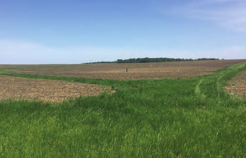
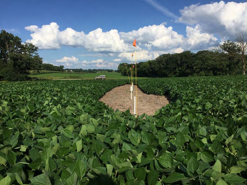
Cover. Photograph showing a piezometer nest, included as part of this study, near Ostrander,
Minnesota. Photograph taken July 2017 by Andrew Berg, U.S. Geological Survey.

Back cover. Photograph showing the south drained site, looking towards the northwest across the
field. Photograph taken June 2017 by Andrew Berg, U.S. Geological Survey.
Potential Groundwater Recharge Rates
for Two Subsurface-Drained Agricultural
Fields, Southeastern Minnesota, 2016–18

By Erik A. Smith and Andrew M. Berg

Prepared in cooperation with the Legislative-Citizen Commission on Minnesota
Resources

Scientific Investigations Report 2020–5006

U.S. Department of the Interior
U.S. Geological Survey
U.S. Department of the Interior DAVID BERNHARDT, Secretary U.S. Geological Survey James F. Reilly II, Director U.S. Geological Survey, Reston, Virginia: 2020 For more information on the USGS—the Federal source for science about the Earth, its natural and living resources, natural hazards, and the environment—visit https://www.usgs.gov or call 1–888–ASK–USGS. For an overview of USGS information products, including maps, imagery, and publications, visit https://store.usgs.gov/. Any use of trade, firm, or product names is for descriptive purposes only and does not imply endorsement by the U.S. Government. Although this information product, for the most part, is in the public domain, it also may contain copyrighted materials as noted in the text. Permission to reproduce copyrighted items must be secured from the copyright owner. Suggested citation: Smith, E.A., and Berg, A.M., 2020, Potential groundwater recharge rates for two subsurface-drained agricultural fields, southeastern Minnesota, 2016–18: U.S. Geological Survey Scientific Investigations Report 2020–5006, 57 p., https://doi.org/10.3133/sir20205006. Associated data for this publication: Smith, E.A., 2020a, DRAINMOD simulations for two agricultural drainage sites in western Fillmore County, southeastern Minnesota: U.S. Geological Survey data release, https://doi.org/10.5066/P987N30U. Smith, E.A., 2020b, Soil-Water Balance model datasets used to estimate recharge for southeastern Minnesota, 2014–2018: U.S. Geological Survey data release, https://doi.org/10.5066/P90N4AWG. Smith, E.A., 2020c, Potential groundwater recharge estimates based on a groundwater rise analysis technique for two agricultural sites in southeastern Minnesota, 2016–2018: U.S. Geological Survey data release, https://doi. org/10.5066/P94LMOPP. U.S. Geological Survey, 2019, USGS groundwater data for Minnesota in USGS water data for the Nation: U.S. Geological Survey National Water Information System database, accessed October 10, 2019, at https://doi. org/10.5066/F7P55KJN. ISSN 2328-0328 (online)

iii

Acknowledgments
Funding for this study was provided by a grant from the Environmental and Natural Resource
Trust Fund of Minnesota (Legislative-Citizen Commission on Minnesota Resources) and from
U.S. Geological Survey Cooperative Matching Funds.

Donald Anderson and James Nelson, both of Ostrander, Minnesota, are greatly acknowledged
for their willingness and cooperation to provide their agricultural fields for this study.

Assistance for securing field-scale monitoring plots included personnel from several State
agencies, including the Minnesota Department of Natural Resources, Minnesota Pollution
Control Agency, and Minnesota Department of Agriculture. Additionally, Beau Kennedy from the
Goodhue Soil and Water Conservation District and Bev Nordby from the Mower Soil and Water
Conservation District were also helpful in early study discussions. Brent Mason, Minnesota
Department of Natural Resources and former U.S. Geological Survey employee, is also
acknowledged for his assistance with installing and removing all piezometers. The authors also
thank Jason Roth of the Natural Resources Conservation Service for a thorough DRAINMOD
model review.

Stephen Kalkhoff and Jared Trost of the U.S. Geological Survey are acknowledged for colleague
reviews of the report. Megan Haserodt and Timothy Cowdery of the U.S. Geological Survey
assisted with model reviews of the Soil-Water-Balance and the RISE Water-Table Fluctuation
models, respectively.
v

Contents
Acknowledgments����������������������������������������������������������������������������������������������������������������������������������������iii
Abstract�����������������������������������������������������������������������������������������������������������������������������������������������������������1
Introduction����������������������������������������������������������������������������������������������������������������������������������������������������2
     Purpose and Scope������������������������������������������������������������������������������������������������������������������������������3
     Previous Studies�����������������������������������������������������������������������������������������������������������������������������������3
     Study Area and Hydrologic Setting���������������������������������������������������������������������������������������������������4
     Climate and Precipitation��������������������������������������������������������������������������������������������������������������������5
     Land Use and Land Cover��������������������������������������������������������������������������������������������������������������������7
Methods����������������������������������������������������������������������������������������������������������������������������������������������������������8
     Site Selection Criteria and Extrapolating Results���������������������������������������������������������������������������8
     Drained and Undrained Monitoring Plots���������������������������������������������������������������������������������������11
     Core Descriptions�������������������������������������������������������������������������������������������������������������������������������11
     Data Sites���������������������������������������������������������������������������������������������������������������������������������������������12
           Soil Volumetric Water Content Sites��������������������������������������������������������������������������������������12
           Groundwater Sites���������������������������������������������������������������������������������������������������������������������13
           Meteorological Sites and Evapotranspiration Calculations�����������������������������������������������14
           Subsurface Drainage Flow Monitoring Sites������������������������������������������������������������������������15
     DRAINMOD Model�����������������������������������������������������������������������������������������������������������������������������16
     Recharge����������������������������������������������������������������������������������������������������������������������������������������������18
           RISE Water-Table Fluctuation Method�����������������������������������������������������������������������������������18
           Soil-Water-Balance Method����������������������������������������������������������������������������������������������������18
Core Descriptions and Unit Interpretations��������������������������������������������������������������������������������������������18
Water-Budget Components—Patterns����������������������������������������������������������������������������������������������������23
     Soil Moisture Conditions�������������������������������������������������������������������������������������������������������������������23
     Evapotranspiration�����������������������������������������������������������������������������������������������������������������������������23
     Water-Table Surface Elevations�������������������������������������������������������������������������������������������������������26
           North Drained Plot���������������������������������������������������������������������������������������������������������������������28
           South Drained Plot���������������������������������������������������������������������������������������������������������������������30
           South Undrained Plot����������������������������������������������������������������������������������������������������������������30
     Subsurface Drainage Flow����������������������������������������������������������������������������������������������������������������30
Potential Groundwater Recharge Rates��������������������������������������������������������������������������������������������������33
     Potential Recharge—RISE Water-Table Fluctuation and Soil-Water-Balance Estimates�����33
     Potential Recharge—DRAINMOD���������������������������������������������������������������������������������������������������39
     Potential Recharge Comparison Across Study Area��������������������������������������������������������������������39
Limitations and Assumptions���������������������������������������������������������������������������������������������������������������������44
Summary�������������������������������������������������������������������������������������������������������������������������������������������������������46
References Cited�����������������������������������������������������������������������������������������������������������������������������������������47
Appendix 1. Instantaneous Subsurface Drainage Flow Rates, Every 15 Minutes, 2017–18��������53
Appendix 2. Daily Total Subsurface Drainage, 2017–18���������������������������������������������������������������������54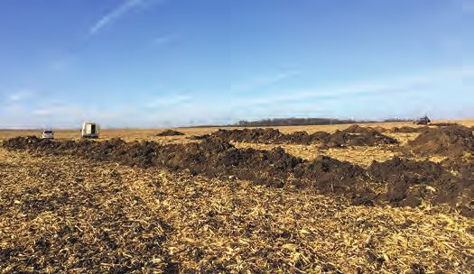
vi
Figures
1. Map showing location of the three field-scale monitoring plots in Fillmore
County, Minnesota������������������������������������������������������������������������������������������������������������������������5
2. Map showing major north drained site locations, including the piezometer
nests, soil moisture probes, meteorological station, and subsurface drainage site��������9
3. Map showing major south drained and undrained plot locations, including the
piezometer nests, soil moisture probes, meteorological station, and subsurface
drainage site��������������������������������������������������������������������������������������������������������������������������������10
4. Map showing land cover in the immediate study area around the two
farmsteads, at a 30-meter resolution, from the 2017 Cropland Data Layers���������������������12
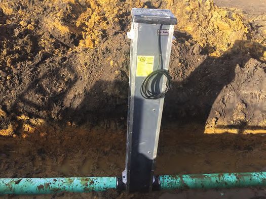
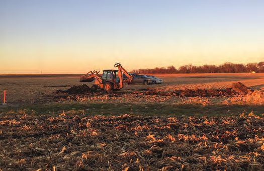
5. Select photographs from the subsurface drain excavation at the south drained
plot, Fillmore County, Minnesota, November 2016............................................................... 13
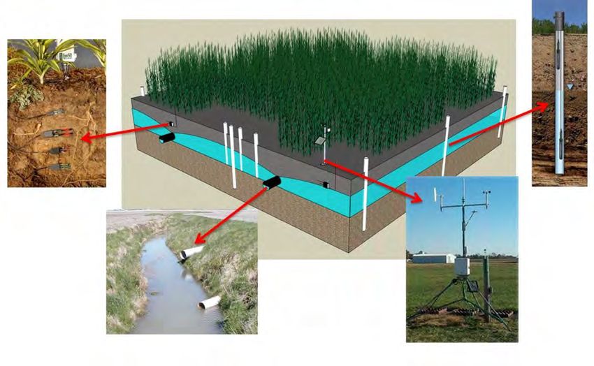
6. A hypothetical configuration of one of the two drained field plots, including
the meteorological station, a piezometer transect for continuous water-level
measurements between two parallel subsurface drains, perimeter piezometers
for background water-level measurements, soil moisture probes, and
subsurface drainage flow���������������������������������������������������������������������������������������������������������14
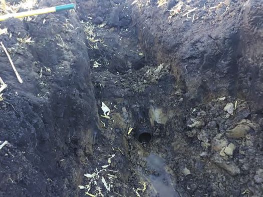
7. Select photographs from the subsurface drain flow monitoring installation at
the north drained plot, Fillmore County, Minnesota, November 2016��������������������������������16
8. Graphs showing volumetric water content for the north drained transects for
October 2016 through September 2018�����������������������������������������������������������������������������������24
9. Graphs showing volumetric water content for the south drained transects and
the south undrained transect from April 2017 through September 2018���������������������������25
10. Graphs showing volumetric water content for the north drained transects, from
June 9 through June 23, 2018���������������������������������������������������������������������������������������������������27
11. Graph showing potential evapotranspiration for both farmsteads, calculated
from the meteorological data at North Site Weather Station and South Site
Weather Station, from June 1 to October 1, 2018������������������������������������������������������������������28
12. Graphs showing water-table surface elevations for the three north drained
transects from December 2016 through September 2018����������������������������������������������������29
13. Graphs showing water-table surface elevations for the two drained transects
and the one undrained transect at the south farmstead from March 2017
through September 2018������������������������������������������������������������������������������������������������������������31
14. Graph showing total subsurface drainage flow, in inches per day, for the North
Site Agri Drain and the South Site Agri Drain from April 1 to July 15, 2018����������������������33
15. Graphs showing simulated and observed water-table surface elevation for
two of the nine DRAINMOD model scenarios from March 1, 2017, to October 1,
2018: STR2–2 and NPR–4�����������������������������������������������������������������������������������������������������������45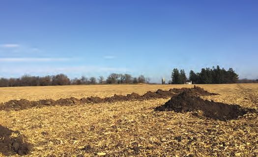
vii

Tables
    1.   Continuous and discrete piezometer network, including piezometer
         identification, transect array, site number, latitude/longitude, land surface
         altitude, screen intervals, and well depths������������������������������������������������������������������������������6
    2.   Non-piezometer data collection across the three monitoring plots, including
         soil moisture, subsurface drainage flow, and meteorological data�������������������������������������8
    3.   Distribution of land cover in the study area, based on the 2017 Cropland
         Data Layers����������������������������������������������������������������������������������������������������������������������������������11
    4.   Grain size distributions for all seven cores across the three monitoring
         plots. Also included is the depth range, textural analysis, U.S. Department of
         Agriculture texture, and the interpreted deposit type����������������������������������������������������������20
    5.   Summary statistics, including minimum, maximum, mean, and median
         volumetric water content for the north drained plot transects, south drained
         plot transects, and the south undrained plot�������������������������������������������������������������������������26
    6.   Total subsurface drainage flow and precipitation, by month, from April 2017
         through October 2018�����������������������������������������������������������������������������������������������������������������32
    7.   Calculated groundwater recharge rates for water year 2017 based on the
         RISE program�������������������������������������������������������������������������������������������������������������������������������34
    8.   Calculated groundwater recharge rates for water year 2018 based on the
         RISE program�������������������������������������������������������������������������������������������������������������������������������36
    9.   Summary statistics, including minimum, maximum, mean, and median potential
         recharge as calculated by the RISE program for water years 2017 and 2018,
         grouped by different categories of piezometer records������������������������������������������������������38
   10.   Model parameters used for the nine DRAINMOD model scenarios discussed in
         this report, summarized by individual DRAINMOD model scenario����������������������������������40
   11.   Potential recharge rate and two calibration statistics for the nine DRAINMOD
         model scenarios completed across the study area��������������������������������������������������������������44
   12.   Annual potential recharge rates based on the DRAINMOD model and RISE
         Water-Table Fluctuation method, grouped by water year���������������������������������������������������46
viii
Conversion Factors
U.S. customary units to International System of Units
Multiply By To obtain
Length
inch (in.) 25.4 millimeter (mm)
foot (ft) 0.3048 meter (m)
mile (mi) 1.609 kilometer (km)
Area
square foot (ft2) 0.09290 square meter (m2)
acre 4,046.86 square meter (m3)
square mile (mi2) 2.590 square kilometer (km2)
Volume
cubic foot (ft3) 0.02832 cubic meter (m3)
Flow rate
foot per second (ft/s) 0.3048 meter per second (m/s)
inch per day (in/day) 2.54 centimeter per day (cm/day)
cubic foot per second (ft3/s) 0.02832 cubic meter per second (m3/s)
Pressure
atmosphere, standard (atm) 101.3 kilopascal (kPa)
Energy
kilowatt hour (kWh) 3,600,000 joule (J)
Hydraulic conductivity
foot per day (ft/d) 0.3048 meter per day (m/d)
Temperature in degrees Celsius (°C) may be converted to degrees Fahrenheit (°F) as follows:
°F = (1.8 × °C) + 32.
Temperature in degrees Fahrenheit (°F) may be converted to degrees Celsius (°C) as follows:
°C = (°F – 32) / 1.8.
Datum
Vertical coordinate information is referenced to the North American Vertical Datum of 1988
(NAVD 88).
Horizontal coordinate information is referenced to the North American Datum of 1983 (NAD 83).
Elevation, as used in this report, refers to distance above the vertical datum.
Supplemental Information
A water year is the 12-month period October 1, for any given year through September 30, of the
following year.ix Abbreviations AV area velocity DEM digital elevation model ET evapotranspiration ET0 potential evapotranspiration MAE mean absolute error MDA Minnesota Department of Agriculture MGS Minnesota Geological Survey NLCD National Land Cover Database NSAD North Site Agri Drain NSI Nash-Sutcliffe index of efficiency NWIS National Water Information System PVC polyvinyl chloride R2 coefficient of determination SSAD South Site Agri Drain SSURGO Soil Survey Geographic SSWS South Site Weather Station SWB Soil-Water-Balance USGS U.S. Geological Survey VWC volumetric water content WTF Water-Table Fluctuation
Potential Groundwater Recharge Rates for Two
Subsurface-Drained Agricultural Fields, Southeastern
Minnesota, 2016–18

By Erik A. Smith and Andrew M. Berg

                                                                   drained monitoring plots had an elevation gradient parallel to
Abstract                                                           the pattern tiles, sloping downward towards the collector drain
                                                                   that aggregated the parallel lines into a single drain. Because
      Subsurface drainage is used to efficiently drain saturated
                                                                   the transects were set at different gradients in the field, some
soils to support productive agriculture in poorly drained ter-
                                                                   of the water-table surface elevation differences were also
rains. Although subsurface drainage alters the water balance
                                                                   attributed to lateral flow towards the lowest parts of the field.
for agricultural fields, its effect on groundwater resources and         Three methods were used to derive potential ground-
groundwater recharge is poorly understood. In Minnesota,           water recharge rates: the RISE WTF method, the USGS
subsurface drainage has begun to increase in southeastern          SWB model, and DRAINMOD-derived deep seepage rates.
Minnesota, even though this part of the State is underlain by      Potential groundwater recharge rates, using the RISE WTF
permeable karstic bedrock aquifers with only a thin layer of       method, across all piezometers were 1.55 and 1.94 inches
glacial sediments separating these aquifers from land surface.     per year, respectively, for water years 2017 and 2018. More
      To gain a better understanding of groundwater recharge       differentiation of potential recharge rates between different
effects from subsurface drainage, the U.S. Geological              piezometer types occurred for water year 2018. Although the
Survey (USGS), in cooperation with the Legislative-Citizen         difference was slightly more than 1 inch between the drained
Commission on Minnesota Resources, led a 2-year hydrologic         and nondrained piezometers for water year 2018, this dif-
study to investigate this connection for two agricultural fields   ference was statistically significant based on a t-test with a
in southeastern Minnesota with subsurface drainage. A total        p-value of 0.036 (α=0.05). When looking at recharge based
of three monitoring plots were used between the two agricul-       on distance from the drain, the subsurface drain did not affect
tural fields: two monitoring plots that included an actively       potential recharge, although other factors such as variability
drained area with peripheral, undrained areas, and a third         in screen depths, well construction, and specific yield vari-
monitoring plot without any subsurface drainage. Multiple          ability cannot be eliminated. The SWB model was also used
piezometer transects were set up across the three monitoring       to estimate potential recharge rates for water years 2017–18,
plots to characterize the unsaturated zone and shallow water-      with rates between 2.44 and 5.92 inches per year for the two
table flow using pressure transducers and soil moisture probes.    drained sites, generally higher than the RISE WTF estimates.
From these piezometers, groundwater recharge rates were            DRAINMOD-derived potential recharge rates were generally
derived using two different methods: the RISE Water-Table          the highest of the three methods, with potential recharge rates
Fluctuation (WTF) method and the DRAINMOD model. In                varying from 2.07 to 9.49 inches per year.
addition to these two methods, the USGS Soil-Water-Balance               Overall, there was a lack of agreement between the three
(SWB) model was used to estimate potential recharge rates for      methods. These results were not remarkable, considering the
three different monitoring plots.                                  fundamental differences in the methodology for each method.
      In addition to deriving groundwater recharge rates, the      However, all methods did show a fundamental difference
hydrologic budget was analyzed to interpret the water-table        between piezometers within the drained area and piezometers
surface elevation and soil volumetric water content time           outside the drained area, including the third undrained moni-
series. At one of the two drained plots, the transects exhibited   toring plot. The drained areas show a lower overall potential
varying water-table surface elevation patterns. Frequent back-     groundwater recharge compared to the nondrained areas for all
flow from the adjacent ditch caused subsurface drainage flow       three estimates. The difference for the 2018 recharge estimates
to slow down or stop drainage through the main collector drain     was slightly higher than 1 inch for the RISE WTF method,
and cause pipe pressurization, so the closest transect appeared    the difference was almost double for the nine sites for the
to be mostly controlled by the drain pressurization, whereas       DRAINMOD model, and the difference between the drain and
the farthest transect was more efficiently drained. Both of the    undrained plots was even more significant for the SWB model.
2 Potential Groundwater Recharge Rates for Two Subsurface-Drained Agricultural Fields, Southeastern Minnesota, 2016–18
Introduction water logging that can impair root proliferation, function, and
metabolism because of saturated soil conditions (Fausey and
In the recently glaciated areas of the upper Midwestern others, 1987; Kanwar and others, 1998). Subsurface drainage
United States (eastern North Dakota, northeastern South also improves soil health by permitting biological processes
Dakota, western and southern Minnesota, and north-central that require the presence of oxygen (Moebius-Clune and
Iowa), the abundant use of artificial surface and subsur- others, 2017). Subsurface drainage also dries out the fields to
face drainage networks has substantially altered the hydro- allow for timely farm operations such as tiling, planting, and
logical conditions from its pre-developed, post-glacial state weed management (Beauchamp, 1987).
(Beauchamp, 1987; Zucker and Brown, 1998). Because the Agricultural drainage has also been connected to sev-
modern landscape of this region is largely a remnant of the eral environmental effects on water quality and water quan-
last glaciation (Wright, 1972), it stands to reason the underly- tity (Blann and others, 2009). The environmental effects on
ing hydrology is also affected by this glaciation and the till surface water quality in particular are well-documented (for
and outwash sediments left behind. Much of this region is example, Dinnes and others, 2002; Kladivko and others, 2004;
low relief, containing many topographic depressions (prai- Richards and others, 2008; Rozemeijer and others, 2010).
rie potholes) underlain by poorly drained soils (Roth and The Gulf of Mexico hypoxia zone, caused mainly by exces-
Capel, 2012). sive nitrogen export through the Mississippi/Atchafalaya
Before this poorly drained landscape could be effectively River Basin, has been connected back to agricultural basins
cultivated for productive agriculture, a land transformation with a high percentage of agricultural drainage (Goolsby and
had to take place that began with the construction of extensive Battaglin, 2001; Randall and Mulla, 2001). Artificial drainage
networks of surface drainage ditches (Wilson, 2016; Capel and networks have also been correlated to watersheds that exhib-
others, 2018). In Minnesota, some of the earliest efforts began ited seasonal and annual water yield increases of greater than
in the Red River Valley of western Minnesota with the forma- 50 percent since 1940 (Schottler and others, 2013).
tion of the Red River Drainage Commission in 1893 (Hanson, The connection of agricultural subsurface drainage to
1987; Smith and others, 2018a). Similar types of drainage dis- changes in groundwater quantity, and the rate of replenishment
tricts sprang up in other parts of Minnesota during this period through groundwater recharge, has not been well-established.
and continued into the early 20th century. Currently (2019), few studies have been carried out to docu-
Along with the construction of surface ditch networks, ment the shifts in the water balance caused by subsurface
drainage practices eventually evolved towards the inclu- drainage (Schuh, 2008). By design, subsurface drainage
sion of artificial subsurface drainage networks (Blann and expedites the movement of water from fields to nearby surface
others, 2009; Capel and others, 2018). Artificial subsurface water bodies.
drainage is the practice of installing networks of perforated In Minnesota, drainage has historically been imple-
conduit below the land surface to drain the upper soil horizons mented in the south-central and western portions of the State,
of excess moisture. Subsurface drainage networks include which are regions underlain primarily by thick impermeable
single field, topographically located drains to patterned drain glacial sediments (Hobbs and Goebel, 1982). Because of the
networks, spanning from a single field to multifield networks. impermeable nature of these glacial sediments, it has often
The subsurface drains typically discharge into an adjacent been assumed that the natural, pre-drained rate of groundwa-
stream or ditch, or connect to a larger publicly maintained ter recharge to aquifers below these glacial sediments was
subsurface drain network that carries the water to the nearest so minimal that the net effect of the installation of subsur-
stream. Early on, subsurface drainage consisted of clay and face drainage networks had a negligible effect on recharge
concrete tile laid out by hand in a narrow, subsequently back- (Schuh, 2008). Recently, though, due to shifts in climatic
filled trench, but eventually the installation practice evolved and economic factors, installation of subsurface drainage
towards the mechanical installation of perforated polyethylene networks has begun to increase in southeastern Minnesota
plastic (Reeve and others, 1981). The installation of subsur- (Smith and others, 2018a). Unlike historically drained regions
face drainage networks continues through present day (2019) of the State, much of southeast Minnesota is underlain by
in Minnesota. thin glacial sediments, often less than 25 feet thick, layered
Subsurface drainage has become an essential component over permeable karstic bedrock aquifers (Runkel and others,
of Minnesota agriculture and other parts of the upper Midwest, 2003). Given consideration of the decreased thickness of the
making row-crop agriculture possible in areas that would glacial sediments covering these bedrock aquifers in southeast
likely suffer from lower yields or would not be economically Minnesota, the prevailing assumption that subsurface drainage
viable (Fausey and others, 1987; Zucker and Brown, 1998). has a minimal effect on groundwater recharge deserves further
More than 25 percent of the croplands of the United States consideration.
require improved drainage (Green and others, 2006). Where Before assumptions can be made about subsurface drain-
agricultural drainage has been installed in Minnesota, its age effects on groundwater recharge, more studies need to be
primary role is to generally lower the water table and effec- carried out. Previously (Fisher and Healy, 2008), water bud-
tively drain ponded surface water. With proper drainage, crop gets of agricultural fields were one possible method for deter-
production can be better managed through the prevention of mining subsurface drainage effects on groundwater recharge.Introduction 3
For a full agricultural field water budget with subsurface Previous Studies
drainage, typical of southeastern Minnesota, all the inputs,
outputs, and rates of change in the area of interest would need Previous hydrogeologic investigations have described the
to be fully examined. In this case, a comprehensive water bud- karst terrain of southeastern Minnesota and the karst aquifers
get would require a full quantification of the changes in water that underlie a high proportion of southeastern Minnesota.
storage for the shallow soils above the restricting layer to the Runkel and others (2003) completed a comprehensive assess-
aquifer below, including evapotranspiration (ET), surface ment of the Paleozoic bedrock hydrogeology for southeastern
runoff, the amount of water drained, and the deeper infiltration Minnesota. Other studies have highlighted the heterogeneity
as groundwater recharge. However, even with accurate mea- of hydraulic properties for these karst aquifers (Tipping and
surements of most of these fluxes, the residual groundwater others, 2006), the complexity of flow patterns from the land
recharge can be difficult to ascertain (Healy and others, 2007; surface to the aquifers (Green and others, 2012), and the sus-
Schuh, 2008; Smith and Westenbroek, 2015). ceptibility of these aquifers to pollution (St. Ores and others,
In an effort to gain a better understanding of ground- 1982). A vast number of other publications have also focused
water recharge effects from agricultural drainage, the on the region (for example, Williams and Vondracek, 2010;
U.S. Geological Survey (USGS), in cooperation with the Groten and Alexander, 2013; Keeler and Polasky, 2014), given
Legislative-Citizen Commission on Minnesota Resources, the distinction that the region’s aquifers bear approximately
led a 2-year hydrologic investigation of two separate field 75 percent of all groundwater in Minnesota (St. Ores and oth-
sites in southeastern Minnesota. The study objective was to ers, 1982).
understand the effect that agricultural subsurface drainage Groundwater recharge in southeastern Minnesota has
might have on water infiltration below the root zone and on been estimated in several studies. Delin (1991) delineated
the overall potential groundwater recharge rates. Through field recharge rates as part of a groundwater-flow study for the
data collection, analysis, and numerical modeling, this study region surrounding Rochester, Minnesota, approximately
considered whether subsurface drainage had an appreciable 30 miles from the study area. Lindgren (2001) also focused
effect on groundwater recharge rates for two agricultural field on groundwater flow and defined recharge rates surrounding
sites. These field sites included two drained plots and one Rochester, Minn. Statewide, several groundwater recharge
undrained plot, with comparisons made between the three estimates have been completed in the past 15 years. Lorenz
different plots. The overall study objective was to measure and Delin (2007) estimated the mean annual recharge from
various water-budget components to isolate groundwater 1971 to 2000, Smith and Westenbroek (2015) estimated the
recharge rates underneath agricultural fields with and without mean annual recharge from 1996 to 2010, and Trost and oth-
subsurface drainage. These groundwater recharge rates would ers (2018) estimated the mean annual recharge from 1980 to
help inform the knowledge gap on how much recharge to the 2011 for the entire glacial aquifer system east of the Rocky
underlying bedrock is affected by agricultural drainage. Mountains.
Potential groundwater recharge studies for southeastern
Minnesota in relation to subsurface drainage do not cur-
Purpose and Scope rently exist. In fact, possible agricultural drainage effects on
groundwater recharge have been rarely studied (Smith and
The purpose of this report is to describe potential ground- others, 2018a). To date, one of the best known studies on this
water recharge rates for two subsurface-drained agricultural topic was carried out in eastern North Dakota to assess the
fields in southeastern Minnesota, 2016–18. This report also potential effects of subsurface drainage on water appropria-
describes the establishment of field-scale monitoring plots tion (Schuh, 2008, 2018). For eastern North Dakota, Schuh
in the two separate agricultural fields with active subsur- (2008) concluded that subsurface drainage might change the
face drains. All monitored plots had various water-budget local groundwater recharge regime, but these cases would be
components continuously monitored for 2 years. Subsurface rare. The study elaborated that subsurface-drained water is
drain flow was continuously monitored with varying success generally removed from an upper zone of active storage that
from the two plots with active subsurface drainage. For both is not considered long-term storage. However, the study also
drained plots, the subsurface drains were all perforated poly- indicated the recharge processes to confined aquifers with
ethylene plastic, often colloquially referred to as tile drains. small hydraulic gradients can be highly sensitive to small
Additionally, each monitoring plot had extensive piezometer water-table changes, such as shifts in water tables caused by
networks to characterize shallow water-table flow and soil subsurface drainage.
moisture probes for unsaturated zone characterization. In total, Rather than direct studies of groundwater recharge,
the two agricultural fields each had a field-scale monitoring partial or complete water budgets in drained systems are
plot with subsurface drains, with a third monitoring plot estab- another source for understanding subsurface drainage effects
lished within an undrained portion of one of the two fields. In on groundwater recharge. Roth and Capel (2012) studied
addition to the continuous monitoring, numerical modeling the water balance of a topographic depression (also termed
was used to quantify potential groundwater recharge rates a “prairie pothole”) and determined that the perched water
across the monitoring plots. table was the groundwater source to the pothole when soils4 Potential Groundwater Recharge Rates for Two Subsurface-Drained Agricultural Fields, Southeastern Minnesota, 2016–18
were saturated, whereas the water in the pothole infiltrated collection sites, including piezometers collecting continu-
to the subsurface drain when soils were drier. DRAINMOD ous water levels, soil moisture probes, a subsurface drainage
was used in the Red River Basin (northwest Minnesota) for flow monitoring station, and a meteorological station (tables 1
several different soil types and it was determined that deep and 2). The total study area for the north drained plot was
seepage to groundwater accounted for a very small percentage, estimated at approximately 6.3 acres, based on the detection of
approximately 1 to 3 percent, of the overall water budget (Jin eight 4-inch diameter parallel drains in the field running east
and others, 2004). Fisher and Healy (2008) determined that to west, with a single 6-inch diameter collector drain running
groundwater recharge was enhanced by subsurface drainage from north to south before heading southwest to the surface
for an Indiana site, as the subsurface drains enhanced recharge ditch. On the western boundary of the north drained plot, the
by reducing surface runoff and inducing water infiltration. flow from the adjacent surface ditch flows under the road
However, agricultural water budgets can be difficult to through a narrow culvert less than 2 meters in width. Because
accurately quantify, largely due to substantial variations in this section of ditch receives extensive drainage from north of
ET rates. Yang and others (2017) determined that subsurface the monitoring plot, in combination with a potentially under-
drainage slightly decreases ET overall on an annual basis, sized culvert, ditch water flow was often slow or completely
with elevated ET during peak growing season on row-cropped stagnant and therefore periodically backed up into the field.
fields, but these fields had lower ET during early spring, fall, Additionally, because this led to the subsurface drains off of
and other fallow periods. However, ET rates for corn and the field to also back up, the field’s drainage capacity was
soybean fields in southeastern North Dakota were determined occasionally exceeded. In these cases, surface runoff would
to be slightly higher in subsurface-drained fields (Rijal and flow directly off of the field towards the ditch or pond in the
others, 2012) for a 2-year period, and Khand and others field.
(2017) found no statistically significant difference in daily The south drained and undrained plots also drained
ET between drained and undrained fields. In all three of these towards Beaver Creek but through a different Beaver Creek
examples, the studies explore the interplay between ET and branch than the north drained plot (fig. 3). Similar to the
subsurface drainage, and do not explore the effects on deep north drained plot, the south drained and undrained plots
seepage or groundwater recharge. contained piezometers collecting continuous water levels
and soil moisture probes, with a subsurface drainage flow
monitoring station and a meteorological station as part of the
Study Area and Hydrologic Setting drained plot (tables 1 and 2). For the south drained plot, all
subsurface drainage was linked to Beaver Creek through an
All three monitoring plots for this study were in Fillmore approximately 600–700-foot section of subsurface drain that
County, Minn., in southeast Minnesota (fig. 1). Two different tied together several properties (not shown on fig. 3). The
farmsteads were used; one of the two drained plots, (the north total study area for the south drained plot was estimated at
drained plot) was located on one farmstead, whereas the other approximately 7.4 acres, based on the detection of three 4-inch
two monitoring plots (the south drained and south undrained diameter parallel drains in the field running approximately
plots) were on the other farmstead. Agreements were secured north to south, with a single 6-inch diameter collector drain
with both landowners to allow for access and the installa- running from northwest to southeast before heading towards
tion of all piezometers, soil moisture probes, meteorological the road culvert. Close to the road culvert, the collector drain
stations, and the subsurface drain sites. These fields were supposedly joined the larger subsurface drain that tied together
selected due to their characteristics typical of the region, such several properties, although this was not physically confirmed.
as shallow depth to bedrock, soil types common for subsurface Surface runoff at the south drained plot tended to move
drainage, low slopes, and established subsurface drainage. towards the lower buffer areas shown in the middle of the
Fillmore County is on the western edge of southeastern south drained plot (fig. 3). For the third monitoring plot, the
Minnesota. Recently, this region of Minnesota has seen an south undrained plot, no actual estimate of the study area was
increase in drainage (Smith and others, 2018a). Unfortunately, necessary because it was not underlain by subsurface drains,
no corroborating documentation of subsurface drainage tiling although for reference the approximate size of the delineated
magnitude has been found for this report aside from these subfield was 2.7 acres.
interviews. Physiographically, both agricultural fields were within an
The north and south farmsteads discharge all subsurface area of southeastern Minnesota that was glaciated (Runkel and
drain flow from the extent of their properties either directly others, 2003). The glacial deposits in general range from less
or indirectly (via a connected surface ditch) to Beaver Creek, than 10 to more than 75 meters in thickness and mainly consist
a tributary to the Upper Iowa River (fig. 1; not shown). As of till with interbedded sand and gravel lens. These deposits
typical for this part of the State, major modifications have overlie bedrock aquifers that consist of Paleozoic sandstone
been made to the natural hydrology of the area. At the north and carbonate aquifers, interstratified by low permeability car-
drained plot (fig. 2), a surface ditch is located adjacent to the bonates and shales (Mossler, 1995; Runkel and others, 2003).
property that drains into Beaver Creek approximately 1 mile These thin till layers are the general location of subsurface
downstream. The north drained plot contained various data drainage in southeastern Minnesota.Introduction 5
92°27' 92°26' 92°25'
EXPLANATION
North drained site
South drained site
South undrained site
43°35'
Bea
ve
r eek
Beaver Cr
FILLMORE COUNTY
Cr
MOWER COUNTY
eek
43°34'
WISCONSIN
ek
re
er C
Beav
MINNESOTA
43°33'
OLMSTED
MOWER FILLMORE
Study
area
IOWA
Base modified from U.S. Geological Survey 0 0.5 1 MILE
and other digital data, various scales
Universal Transverse Mercator Projection, zone 15 North 0 0.5 1 KILOMETER
North American Datum of 1983
Figure 1. Location of the three field-scale monitoring plots (two drained plots, one undrained plot) in Fillmore County, Minnesota.
Beaver Creek and some of the connecting surface ditches are also shown.
To obtain specific information for this study, seven Conservation Service SSURGO data, included Floyd silty clay
complete cores were sent to the Minnesota Geological Survey loam, Clyde silty clay loam, Kasson silt loam, Kenyon silt
(MGS) for full descriptions: four of the sediment cores were loam, and Renova silt loam (Natural Resources Conservation
from the north drained plot, two from the south drained plot, Service, 2019).
and a single core from the south undrained plot. These cores
confirmed that most of these fields were underlain by vari-
ous till complexes, outwash deposits, and loess. The textures Climate and Precipitation
from the cores mostly clustered as loam, clay loam, and
silty clays with a few notable exceptions. More details on The climate of the study area is humid continental, with
the cores are available in the “Core Descriptions and Unit warm, humid summers and cold winters with heavy snow-
Interpretations” section. Soils for the three monitoring plots fall. Climate data from the Rochester International Airport
were developed under long-grass prairies on the glacial till (not shown; National Climatic Data Center, 2019), about
deposits and are highly productive (Cowles and others, 1958). 24–28 miles north of the study area (north drained plot,
Major soils present at the plots, based on Natural Resources 24 miles; south drained/undrained plots, 28 miles), had a long6 Potential Groundwater Recharge Rates for Two Subsurface-Drained Agricultural Fields, Southeastern Minnesota, 2016–18
Table 1. Continuous and discrete piezometer network, including piezometer identification (short name), transect array (if applicable),
site number, latitude/longitude, land surface altitude, screen intervals, and well depths.
[ID, identification; USGS, U.S. Geological Survey; --, nontransect]
Continuous Land
Piezometer USGS site Screened Well
Transect (C) 2 or Latitude3 Longitude3 surface
ID1 ID number interval5 depth5
Discrete (D) altitude4
NTR1–1 NTR1 433527092265501 C 43.59088 −92.44873 1,334.95 1.89–6.36 7.1
NTR1–2 NTR1 433527092265502 C 43.59093 −92.44872 1,335.23 1.90–6.37 7.1
NTR1–3 NTR1 433527092265503 C 43.59098 −92.44871 1,334.99 2.92–7.39 8.1
NTR1–4 NTR1 433527092265504 C 43.59103 −92.44871 1,334.93 1.95–6.42 7.1
NTR1–5 NTR1 433527092265505 C 43.59109 −92.44871 1,334.79 1.89–6.36 7.1
NTR2–1 NTR2 433528092265101 C 43.59112 −92.44750 1,339.27 3.12–7.59 8.3
NTR2–2 NTR2 433528092265102 C 43.59116 −92.44750 1,339.30 3.17–7.64 8.3
NTR2–3A NTR2 433528092265103 C 43.59121 −92.44750 1,339.53 2.69–4.73 5.3
NTR2–3B NTR2 433528092265104 C 43.59121 −92.44749 1,339.59 3.65–10.58 11.3
NTR2–3C NTR2 433528092265105 D 43.59121 −92.44749 1,339.41 15.75–25.22 25.9
NTR2–3D NTR2 433528092265106 C 43.59119 −92.44750 1,339.55 30.14–31.10 31.2
NTR2–4 NTR2 433528092265107 C 43.59126 −92.44749 1,339.52 3.22–7.69 8.4
NTR2–5 NTR2 433528092265108 C 43.59131 −92.44749 1,339.38 3.17–7.64 8.3
NTR3–1 NTR3 433531092265301 C 43.59199 −92.44797 1,339.18 3.72–8.19 8.9
NTR3–2 NTR3 433531092265302 D 43.59204 −92.44797 1,339.20 3.17–7.64 8.3
NTR3–3A NTR3 433531092265303 C 43.59209 −92.44797 1,339.39 3.17–7.64 8.3
NTR3–3B NTR3 433531092265304 C 43.59209 −92.44796 1,339.38 4.40–11.33 12.0
NTR3–4 NTR3 433531092265305 D 43.59214 −92.44796 1,339.43 3.17–7.64 8.3
NTR3–5 NTR3 433531092265306 C 43.59219 −92.44796 1,339.49 3.17–7.64 8.3
NPR–1 -- 433533092264901 C 43.59238 −92.44701 1,342.01 6.69–13.65 14.3
NPR–2 -- 433533092265701 C 43.59256 −92.44906 1,335.38 7.49–14.42 15.1
NPR–3 -- 433530092265701 D 43.59163 −92.44909 1,334.60 5.84–15.30 21.00
NPR–4 -- 433527092265701 C 43.59096 −92.44908 1,334.15 3.36–12.82 15.9
NPR–5 -- 433531092263901 C 43.59196 −92.44405 1,346.80 3.38–15.31 16.00
STR1–1 STR1 433247092260701 C 43.54649 −92.43527 1,293.44 4.98–9.46 10.0
STR1–2 STR1 433247092260702 C 43.54649 −92.43533 1,293.20 4.98–9.46 10.0
STR1–3A STR1 433247092260703 C 43.54649 −92.43541 1,293.14 4.61–9.29 9.9
STR1–3B STR1 433247092260704 C 43.54649 −92.43541 1,293.09 8.43–12.91 13.5
STR1–4 STR1 433247092260705 C 43.54648 −92.43549 1,292.95 4.65–9.13 9.7
STR1–5 STR1 433247092260706 C 43.54648 −92.43555 1,292.82 4.98–9.47 10.0
STR2–1 STR2 433243092260601 C 43.54538 −92.43494 1,284.58 4.92–9.40 10.0
STR2–2 STR2 433243092260602 C 43.54538 −92.43501 1,284.75 4.90–9.38 10.0
STR2–3A STR2 433243092260603 C 43.54538 −92.43509 1,284.97 4.83–9.31 9.9
STR2–3B STR2 433243092260604 D 43.54538 −92.43509 1,284.92 6.54–11.02 11.6
STR2–4 STR2 433243092260605 C 43.54538 −92.43516 1,285.00 4.94–9.42 10.0
STR2–5 STR2 433243092260606 C 43.54538 −92.43523 1,285.06 4.93–9.41 10.0
SUTR1–1 SUTR1 433245092254901 D 43.54591 −92.43024 1,286.88 1.75–3.74 4.3
SUTR1–2 SUTR1 433245092254902 D 43.54591 −92.43031 1,287.23 4.39–8.87 9.4
SUTR1–3 SUTR1 433245092254903 D 43.54592 −92.43039 1,287.62 2.92–7.40 8.0
SUTR1–4 SUTR1 433245092254904 C 43.54592 −92.43046 1,287.98 4.40–8.88 9.3
SUTR1–5 SUTR1 433245092254905 C 43.54593 −92.43053 1,288.49 6.98–11.46 12.0Introduction 7
Table 1. Continuous and discrete piezometer network, including piezometer identification (short name), transect array (if applicable),
site number, latitude/longitude, land surface altitude, screen intervals, and well depths.—Continued
[ID, identification; USGS, U.S. Geological Survey; --, nontransect]
Continuous Land
Piezometer USGS site Screened Well
Transect (C) 2 or Latitude3 Longitude3 surface
ID1 ID number interval5 depth5
Discrete (D) altitude4
SUPR–1 -- 433246092254801 C 43.54625 −92.43015 1,283.53 1.73–6.20 6.9
SUPR–2 -- 433246092255001 C 43.54621 −92.43058 1,286.47 2.44–6.91 7.6
SUPR–3 -- 433244092255001 D 43.54562 −92.43065 1,286.88 3.33–7.80 8.5
SUPR–4 -- 433244092255002 C 43.54562 −92.43066 1,291.92 45.91–50.22 50.9
SUPR–5 -- 433244092254901 D 43.54550 −92.43028 1,290.76 2.17–6.65 7.2
SPR–1A -- 433242092260901 C 43.54502 −92.43606 1,283.49 5.01–9.49 10.1
SPR–1B -- 433242092260902 C 43.54501 −92.43607 1,283.61 35.14–39.45 40.1
SPR–2 -- 433249092260801 C 43.54705 −92.43578 1,296.44 9.12–13.60 14.2
SPR–4 -- 433249092260501 C 43.54707 −92.43488 1,301.36 9.84–14.32 14.9
SPR–5 -- 433240092260601 C 43.54471 −92.43468 1,280.29 2.83–7.31 7.9
1The first segment of the piezometer identification includes the piezometer nest (for example, NTR1–1 belongs to NTR1); otherwise, P-label in first segment
(for example, NPR–1) designates a perimeter piezometer.
2Piezometers identified with continuous water-table surface elevations have partial or full water-level records from October 1, 2016, through
September 30, 2018.
3Latitude/longitude in decimal degrees.
4Altitude in feet above the vertical datum, based on North American Vertical Datum 1988 (NAVD 88).
5Screened interval and well depth in feet below land surface.
continuous period of record (1936 to the present) and was to 2018. Additionally, the number of days with more than
useful for putting short-term climate data collected within the 1 inch of precipitation has increased in 1990–2018 com-
study area into historical perspective. Based on this long- pared to the previous period: 5.7 days from 1933 to 1989, but
term record, the mean January temperature was −4.4 degrees 7.5 days from 1990 to 2018.
Celsius (°C) (24 degrees Fahrenheit [°F]), the mean July
temperature was 27.2 °C (81 °F), and the mean annual
Land Use and Land Cover
temperature was 7.3 °C (45.2 °F) (National Climatic Data
Center, 2019). Land use and land cover for the immediate area surround-
Generally, precipitation increases in early spring after ing the two farmsteads were analyzed to obtain an improved
snowmelt from less than 0.8 inch in February to 4.6 inches perspective of the land-use setting. Of the selected area, more
in June. Rain in spring is considered reliable but decreases than 80 percent of the land area was covered by either corn or
throughout the summer. Occasionally, heavy spring rains delay soybean fields (fig. 4; table 3). The rest of the area was divided
crop planting. Annual precipitation rates can vary dramati- between forest, developed land of all types (including roads),
cally between wet and dry periods, ranging from 15.46 inches and grass/pasture land, with a small amount of land devoted
(1976) to 43.98 inches (1990). However, annual precipitation to alfalfa or other hay and peas. These data were obtained
has increased in the past three decades (1990–2018) compared from the 2017 Cropland Data Layers (National Agricultural
to the previous period going back to 1933 (1933–89). The Statistics Service, 2019). Although the various fields would
mean annual precipitation from 1933 to 1989 at the Rochester alternate between corn and soybeans, and occasionally alfalfa
International Airport was 28.9 inches per year, whereas the or other hay, the relative percentages from year to year were
mean annual sum increased to 34.4 inches per year from 1990 largely the same.8 Potential Groundwater Recharge Rates for Two Subsurface-Drained Agricultural Fields, Southeastern Minnesota, 2016–18
Table 2. Non-piezometer data collection across the three monitoring plots, including soil moisture (volumetric water content),
subsurface drainage flow, and meteorological data.
[ID, identification; USGS, U.S. Geological Survey; NSAD, North Site Agri Drain; --, not applicable; SSAD, South Site Agri Drain; NSWS, North Site Weather
Station; SSWS, South Site Weather Station]
Site ID Transect USGS site ID number Latitude1 Longitude1
Soil moisture (volumetric water content)2
NTR1–3 NTR1 433527092265503 43.59098 −92.44871
NTR1–5 NTR1 433527092265505 43.59109 −92.44871
NTR2–3A NTR2 433528092265103 43.59121 −92.44750
NTR2–5 NTR2 433528092265108 43.59131 −92.44749
NTR3–3A NTR3 433531092265303 43.59209 −92.44797
NTR3–5 NTR3 433531092265306 43.59219 −92.44796
STR1–3A STR1 433247092260703 43.54649 −92.43541
STR1–5 STR1 433247092260706 43.54648 −92.43555
STR1–3A STR2 433243092260603 43.54538 −92.43509
STR1–5 STR2 433243092260606 43.54538 −92.43523
SUTR1–3 SUTR1 433245092254903 43.54592 −92.43039
SUTR1–5 SUTR1 433245092254905 43.54593 −92.43053
Subsurface drain flow
NSAD -- 433527092265601 43.59081 −92.44884
SSAD -- 433240092260501 43.54471 −92.43487
Meteorological3
NSWS -- 433531092263902 43.59196 −92.44405
SSWS -- 433241092254601 43.54495 −92.42948
1Latitude/longitude in decimal degrees.
2Each listed soil moisture station included two depths: 1.33 feet and 2.67 feet.
3The meteorological station included the following parameters: air temperature, relative humidity, rainfall, wind speed and direction, and solar radiation.
Methods elevations, and most importantly, deep seepage rates. The deep
seepage rate approximated the expected groundwater recharge
During this study, a large monitoring network was created to the aquifer below the local restricting layer. The complete
to capture the groundwater-related water-budget components DRAINMOD model archives are available as a USGS data
for three monitoring plots (two drained plots, one undrained release (Smith, 2020a). In addition to deriving potential
plot). Within the monitoring network, continuous water-table groundwater recharge rates from the DRAINMOD model, two
surface monitoring, soil volumetric water content monitor- other methods of estimating potential groundwater recharge
ing of the unsaturated zone, and subsurface drainage flow were used: (1) an updated Minnesota Soil-Water-Balance
monitoring data were collected for 2 water years (2017 and (SWB) potential recharge model, and (2) the RISE Water-
2018), plus continuous meteorological monitoring (includ- Table Fluctuation (WTF) method (Rutledge, 1997). In contrast
to the DRAINMOD model, these two methods approximate
ing precipitation) during the same time period. A water year
the amount of recharge to the water table closest to land sur-
is the 12-month period October 1, for any given year through
face. These additional recharge calculations are also available
September 30, of the following year. From a modeling per-
as USGS data releases: the updated Minnesota SWB model
spective, the study focused on the recharge calculations and
(Smith, 2020b) and RISE WTF calculations (Smith, 2020c).
the overall patterns in water-table surface elevations of the
piezometer network.
Three different methods were used to derive groundwater Site Selection Criteria and Extrapolating Results
recharge. DRAINMOD, a field-scale, process-based, distrib-
uted model often used for agricultural fields with subsurface Fields were selected that had patterned subsurface drain-
drainage (Skaggs, 1980; Skaggs and others, 2012), was used age, as these fields generally have subsurface drainage with
to simulate subsurface drainage flow, water-table surface regular spacing, at uniform depths, and all sloping at an equalYou can also read