PRACTICAL ADAPTATION TO CLIMATE CHANGE IN REGIONAL NATURAL RESOURCE MANAGEMENT
←
→
Page content transcription
If your browser does not render page correctly, please read the page content below
Queensland the Smart State

 PRACTICAL ADAPTATION TO CLIMATE CHANGE
 IN REGIONAL NATURAL RESOURCE
 MANAGEMENT

 Queensland Case Studies – South East Queensland
 Western Catchments Report

Australian Greenhouse Office
Sinclair Knight Merz
Queensland Murray Darling Basin Committee
Desert Channels Queensland
Fitzroy Basin Association
South East Queensland Western Catchments

August 2007
PRACTICAL ADAPTATION TO CLIMATE CHANGE IN REGIONAL
NATURAL RESOURCE MANAGEMENT
Investigator:                               Mr David Cobon
                                            Queensland Climate Change Centre of Excellence
                                            Department of Natural Resources and Water
                                            PO Box 318
                                            TOOWOOMBA Q 4350

Project No:      EP08

Qld Case Studies – Report for SEQWC Case Study – Climate Change Impacts on Water Resources of
South-East Queensland Western Catchments

Authors:

Mr David Cobon, Principal Scientist, Climate Change Centre of Excellence, Toowoomba
Mr Nathan Toombs, Research Scientist, Climate Change Centre of Excellence, Toowoomba

Project Team:

Mr David Cobon, Principal Scientist, Climate Change Centre of Excellence, Toowoomba
Mr Nathan Toombs, Research Scientist, Climate Change Centre of Excellence, Toowoomba
Dr Xike Zhang, Research Scientist, Climate Change Centre of Excellence, Toowoomba
Mr Craig Johansen, Principal Scientist, Department of Natural Resources and Water, Indooroopilly

Project Partner Team:

Funding Co-ordinator               Paul Ryan, Australian Greenhouse Office
Project Leader                     Craig Clifton, Sinclair Knight Merz
State Co-ordinator                 Trica Gowdie, Queensland Murray Darling Basin Committee
Catchment Member                   Michael Bent, Fitzroy Basin Association
Catchment Member                   Steve Wilson, Desert Channels Queensland
Catchment Member                   Dave Manning, South East Queensland Western Catchments
Reference Group Members            Paul Ryan, Craig Clifton, Roger Jones, David Poulter, Mirko
                                   Stauffacher, Geoff Park, John Francis, Trica Gowdie, David Cobon

Commencement Date: 1 July 2005                       Completion Date: 30 June 2007

Cover: Water infrastructure and resources in south-east Queensland. Photos courtesy of staff in the Department
of Natural Resources and Water
Published by: Department of Natural Resources and Water, Queensland Climate Change Centre of Excellence,
Toowoomba, 2007

Australian Greenhouse Office                                                                            Page ii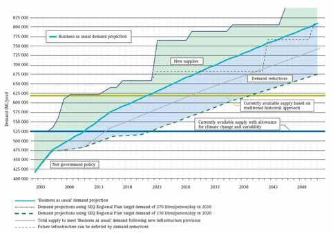
Contents

                                                                                                                                                     Page

Contents................................................................................................................................................ iii

Figures....................................................................................................................................................5

Tables .....................................................................................................................................................7

Executive Summary ...............................................................................................................................8

1      Project overview .............................................................................................................................9

2      Objectives of the case study ...........................................................................................................9

3      South East Queensland Western Catchments ...............................................................................10

4     The climate change scenarios .......................................................................................................12
    4.1 Uncertainity in climate change ................................................................................................12
    4.2 Climate change patterns ..........................................................................................................13
    4.3 Climate change scenarios ........................................................................................................16

5     Model construction and calibration ..............................................................................................17
    5.1 General circulation models......................................................................................................17
    5.2 Perturbing historical data.........................................................................................................17
    5.3 Overview of Sacramento rainfall-runoff model ......................................................................18
    5.4 Model set-up and calibration – Brisbane River system ...........................................................18
    5.5 Application of climate change factors .....................................................................................20

6     Results of impact assessment .......................................................................................................20
    6.1 Annual flow changes ...............................................................................................................20
    6.2 Annual inflows to storages ......................................................................................................21
    6.3 Monthly flow changes .............................................................................................................21
    6.4 Daily flow changes ..................................................................................................................23
    6.5 Low flows................................................................................................................................23
        6.5.1 Duration of low flows..................................................................................................23
        6.5.2 Frequency of low flows ...............................................................................................24
    6.6 High flows ...............................................................................................................................25
        6.6.1 Duration of high flows.................................................................................................25
        6.6.2 Frequency of high flows ..............................................................................................25

Australian Greenhouse Office                                                                                                                       Page iii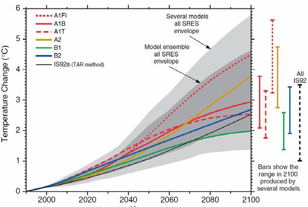
6.7 Environmental flows ...............................................................................................................25

7      Future water demand ....................................................................................................................26

8     Conclusions and recommendations ..............................................................................................28
    8.1 Summary of risk analysis ........................................................................................................28
    8.2 Limitations of the assessment..................................................................................................29
        8.2.1 Greenhouse-related uncertainties.................................................................................29
        8.2.2 Climate model limitations............................................................................................29
        8.2.3 Scenario construction methods ....................................................................................30
        8.2.4 Scenario application.....................................................................................................30
        8.2.5 Climate change and variability ....................................................................................31
        8.2.6 Hydrological uncertainties...........................................................................................31
    8.3 Summary and recommendations .............................................................................................31

9      Acknowledgements ......................................................................................................................32

10 References ....................................................................................................................................32

11 Appendix 1 – Exceedance curve for monthly flows for the Brisbane River downstream of the Mt
Crosby Weir .........................................................................................................................................34

12 Appendix 2 – Average seasonal flows for the Brisbane River downstream of the Mt Crosby Weir
   35

13 Appendix 3 – Frequency plots of low flows for the Brisbane River downstream of the Mt Crosby
Weir......................................................................................................................................................36

14 Appendix 4 – Average annual inflows into major storages..........................................................37

15 Appendix 4 – Maps for wet and dry scenarios for SEQ Western Catchments .............................39
  14.1 Minimum temperature – dry scenario .....................................................................................39
  14.2 Minimum temperature – wet scenario.....................................................................................40
  14.3 Maximum temperature – dry scenario ....................................................................................42
  14.4 Maximum temperature – wet scenario ....................................................................................44
  14.5 Mean temperature – dry scenario ............................................................................................46
  14.6 Mean temperature – wet scenario............................................................................................48
  14.7 Rainfall – dry scenario ............................................................................................................50
  14.8 Rainfall – wet scenario............................................................................................................52
  14.9 Potential evaporation – dry scenario .......................................................................................54
  14.10 Potential evaporation – wet scenario.....................................................................................56

16 Appendix 5 – Simulated flows downstream of Mt Crosby Weir .................................................58

Australian Greenhouse Office                                                                                                                       Page iv
Figures
Page
Figure 1. South East Queensland Western Catchments. ..................................................................... 11
Figure 2. Global mean temperature projections for the six illustrative SRES scenarios using a
simple climate model tuned to a number of complex models with a range of climate
sensitivities. Also for comparison, following the same method, results are shown for
IS92a. The darker shading represents the envelope of the full set of thirty-five SRES
scenarios using the average of the models results. The lighter shading is the envelope
based on all seven model projections (from IPCC, 2001)........................................................... 12
Figure 3. Average monthly percentage change in rainfall and potential evaporation for South
East Queensland Western Catchments (see Table 4 for the 11 locations) per degree of
global warming using the nine climate models and emissions scenarios with medium
sensitivity shown in Table 1 with one standard deviation........................................................... 14
Figure 4. Average monthly percentage change in a) rainfall and b) potential evaporation for
South East Queensland Western Catchments (see Table 4 for the 11 locations) per degree
of global warming for the nine climate models shown in Table 1 at medium (MS) and
high sensitivity (HS).................................................................................................................... 15
Figure 5. Map of Brisbane River system with sub-systems highlighted. The location of the
node used for this analysis (IQQM node 203 – downstream of Mt. Crosby Weir) is also
shown. .................................................................................................................................... 19
Figure 6. Mean annual streamflow of the Brisbane River downstream of Mt Crosby Weir for
the base scenario and the dry and wet climate change scenarios for 2030.................................. 21
Figure 7. Simulated average monthly flow for the Brisbane River downstream of Mt Crosby
Weir for the base, dry and wet scenarios for 2030. ..................................................................... 22
Figure 8. Simulated 12 month moving average flows of the Brisbane River downstream of Mt
Crosby Weir for base conditions and under dry and wet climate change scenarios for
2030. .................................................................................................................................... 22
Figure 9. Daily flow exceedance curves for the base, dry and wet climate change scenarios for
Brisbane River downstream of Mt Crosby Weir in 2030. ........................................................... 23
Figure 10. a) Chance of exceeding duration of low flows (1450 ML/d for the Brisbane River downstream of Mt Crosby Weir for
base scenario and the wet and dry climate change scenarios in 2030. ........................................ 25
Figure 13. Future water demand for industrial and urban use for South East Queensland.
(Source: SEQ Regional Water Supply Strategy - 2nd Interim Report, 2005)............................... 26
Australian Greenhouse Office Page 5Figure 14. Fractions of water supply used by different sectors in South East Queensland
(Source: SEQ Regional Water Supply Strategy - 2nd Interim Report, 2005)............................... 26
Figure 15. Future water demand for industrial and urban use for South East Queensland with
demand reductions and new water supplies. (Source: SEQ Regional Water Supply
Strategy - 2nd Interim Report, 2005) ............................................................................................ 27
Australian Greenhouse Office Page 6Ta b l e s
Page
Table 1. Climate model simulations analysed in this report. The non-CSIRO simulations may
be found at the IPCC Data Distribution Centre (http://ipcc-ddc.cru.uea.ac.uk/). Note that
DARLAM125 and CC50 are regional climate models ............................................................... 13
Table 2. Changes in annual rainfall and point potential evaporation for South East Queensland
Western Catchments, simulated by the models in Table 1, expressed as a percentage
change per degree of global warming.......................................................................................... 14
Table 3. Dry and wet climate change scenarios for 2030 for South East Queensland Western
Catchments .................................................................................................................................. 16
Table 4. Climate stations together with their latitudes and longitudes for which climate
change factors were obtained from OzClim ................................................................................ 17
Table 5. Climate change factors (% change from base scenario) for the dry and wet scenarios
for 2030 over South East Queensland Western Catchments ....................................................... 20
Table 6. Changes in mean annual stream flow of the Brisbane River downstream of Mt
Crosby Weir for the dry and wet climate change scenarios for 2030.......................................... 20
Table 7. Duration of lows flows for the Brisbane River downstream of Mt Crosby Weir for
the base, wet and dry climate change scenarios .......................................................................... 24
Table 8. Periods that existing supplies will meet demand for different levels of domestic
consumption. (Source: SEQ Regional Water Supply Strategy - 2nd Interim Report, 2005)........ 27
Australian Greenhouse Office Page 7Executive Summary
A number of general circulation models (9) and greenhouse gas emission scenarios (3)
were used to provide a range of projected temperature, evaporation and rainfall change to
2030. The wettest and driest climate scenarios for the region were used in hydrological
models to assess changes in water flow for the Brisbane River. Changes in climate, water
flow and water supply were measured against a base period from 1961-1990.
Annual rainfall projections range from slightly wetter, to drier than the historical climate.
Six of the nine models expressed an annual drying trend. Seasonally, changes are uncertain in
DJFM and AMJJ but are dominated by decreases in ASON. Changes in potential evaporation
are much more certain, always increasing and showing a slight inverse relationship with
rainfall.
The dry scenario for 2030 was associated with reduced annual rainfall of 5%, a mean
temperature increase of 1.2oC and higher evaporation of 8%. The wet scenario for 2030
was associated with higher annual rainfall of 2%, a mean temperature increase of 0.8oC
and higher evaporation of 2%.
Based on the set of scenarios, either increases or decreases in stream flow are possible for
the Brisbane River downstream of Mt Crosby Weir depending on which scenario is most
closely associated with observed climate in the future. The change in mean annual flow
ranged from -28% to +14% by 2030. Average annual inflows into Somerset, Wivenhoe and
Mt Crosby storages were 7-10% higher for the wet scenario and 12-20% lower for the dry
scenario.
The dry/wet scenarios were associated with decreased/increased flows for the upper range
(~10-50,000 ML/d) compared to the base scenario. The 60-99 percentile daily flows under the
dry scenario were 20-81% lower than the base scenario. For the wet scenario these flows were
13-67% higher than the base scenario. There was no apparent difference in low and extreme
high daily flows between the base, wet and dry scenarios.
The mean annual frequency of low daily flows (1450 ML/day) at the Brisbane River
downstream of Mt Crosby Weir was lower for the dry scenario, and higher for the wet
scenario, compared to base. The mean numbers of days of high flow per year for the base, wet
and dry scenarios were 36, 41 and 26 days respectively.
The longest simulated duration of low flow (1450 ML/day) was 11 days for the base scenario. There was no difference
(P>0.05) from the base scenario for all scenarios.
The effects of the dry scenario will be magnified by increased water demand from
population and industrial growth in South East Queensland (SEQ). Demand may rise by 35%
by 2030. Water planning processes in SEQ indicate additional urban and industrial supplies
will be needed by 2021. However to account for the risk associated with climate
variability and climate change a 16% reduction in water yield has been allowed for,
reducing the period existing supplies meet demand to 2011. This allowance is likely to be
within the range of reduced water yields reported in this study for the dry scenario. A
Australian Greenhouse Office Page 8wet scenario is likely to extend the period SEQ will need additional urban and industrial
supplies beyond 2021. The capacity to supply sufficient water to SEQ under climate change
conditions requires further investigation.
1 Project overview
The project involved seven regional natural resource management (NRM) organisations -
including the South East Queensland Western Catchments (SEQWC), Queensland Murray-
Darling Basin Committee (QMDC) – and the Queensland Department of Natural Resources
and Water. It was coordinated by Sinclair Knight Merz.
The project has two main objectives, as follows:
1. improve understanding of the implications of climate change for regional NRM
2. develop tools and processes that help regional NRM organisations incorporate
climate change impacts, adaptations and vulnerability into their planning
processes.
The project was divided into three main stages:
Stage A. This stage identified components of participating region’s natural resource
system that were more vulnerable to climate change. The key steps were to develop the
‘conceptual mapping’ workshop process, conduct a literature review to document climate
change projections, impacts and adaptive mechanisms for each participating region and then
to run ‘conceptual mapping’ workshops in each of these regions.
Stage B. This stage completed a series of regional case studies which explored climate
change impacts on one or a small number of components of the natural resource system that
were more vulnerable to climate change. The case studies were designed to provide more
objective information on climate change impacts and vulnerability and will be used to support
analysis of how regional NRM processes can incorporate climate change considerations.
Results of the case study for SEQWC are reported here and will be used by each of the
participating NRM regions to complete Stage C.
Stage C. The final stage, in which lessons from the case study will be used to help
develop tools and processes (e.g. thinking models, numerical models, workshop processes,
modifications to risk assessment processes) that enable regional NRM organisations to
incorporate climate change into their planning, priority setting and implementation. A series
of workshops will be held in each state to receive feedback on the tools and processes
developed or identified through the project.
2 Objectives of the case study
Earlier work in this project (Stage A) completed a review of literature and assessment of
the likely impacts of climate change in South East Queensland (Fry and Willis 2005) and is
available from the SEQWC office in Brisbane or QMDC in Toowoomba. A meeting was held
in Gatton (September 2005) to help the community better understand the drivers, pressures
and impacts of climate change, and to plan the responses that maybe useful to prepare for
climate change (Stage A). During this process a number of key issues were identified related
Australian Greenhouse Office Page 9to climate change (Clifton and Turner 2005). This report provides a scientific assessment
(Stage B) of one key issue in the region, namely; under climate change conditions for 2030
identify changes in:
1. Regional rainfall, temperature and evaporation
2. Surface flow in the upper Brisbane River (Wivenhoe and Somerset Dams) and the
reliability of water supply
3. Future demand of water from agricultural, consumptive and environmental uses.
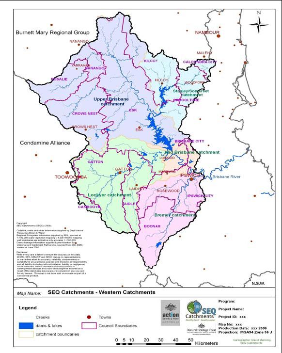
3 South East Queensland Western Catchments
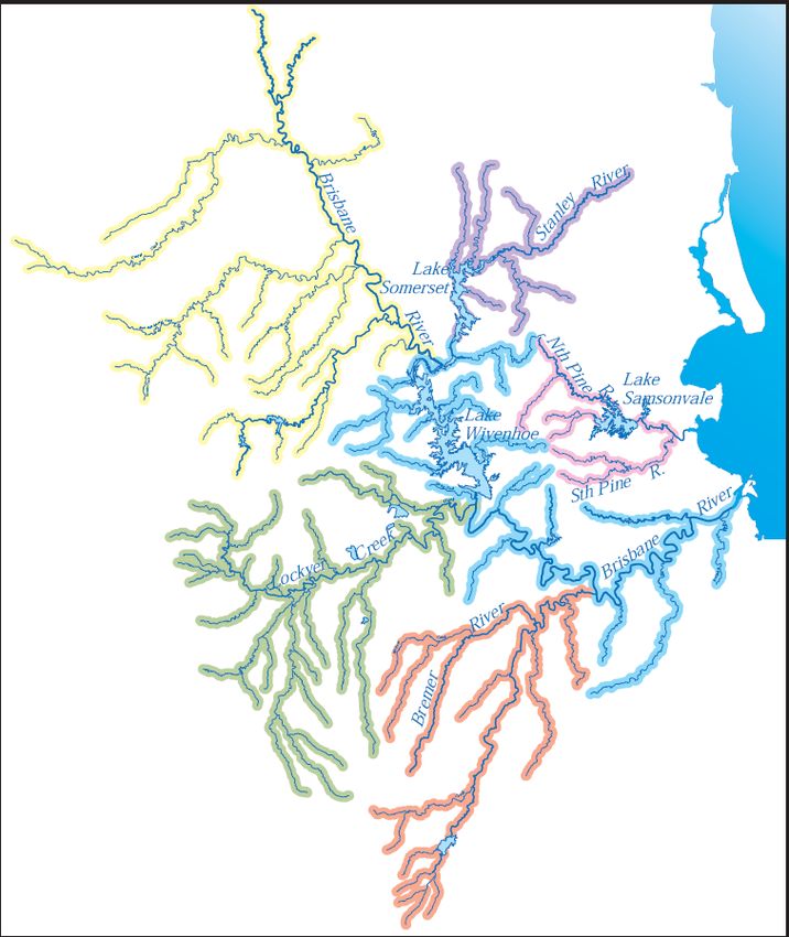
The region’s surface water is a major feature of its landscape. There are a total of thirteen
water bodies in the region, the majority of which are associated with impoundments in
Somerset and Wivenhoe Dams (Figure 1). These dams supply water to well over a million
people in urban centres throughout SEQ, although the majority of people are located outside
the boundaries managed by SEQWC. Likewise, the City of Toowoomba is outside the region,
and is supplied from Perseverance and Cressbrook Dams.
The Brisbane River is bounded by the Great Dividing Range to the west, and the
D’Aguilar Ranges to the east. It rises in the north and flows generally south east to Moreton
Bay.The catchment comprises the upper reaches of five river basins: Somerset-Stanley; Upper
Brisbane – Wivenhoe; Lockyer Valley; Mid-Brisbane Valley; and, the Bremer River. Of
these, the Brisbane River is the main river system.
Land use within the basin is a mixture of state forest, grazing, horticulture, and a large
proportion of urbanised areas. Included in the catchment are the major cities of Brisbane and
Ipswich, and the larger towns of Laidley, Gatton, Esk, Kilcoy, and Woodford.
The predominant land use is the grazing of beef cattle which accounts for approximately
42% of total land area. Grazing also extends into the 36.4% of natural bushland. Managed
forests represent 9.4%, intensive agriculture 4.8% (producing a significant proportion of
Queensland’s vegetable crop), and 1.2% is formally protected conservation area. The
remaining 6.2% accommodates all other activities, including urban development and
industrial areas. Urban water supply is the major use of water within the catchment.
There are two significant supplemented irrigation schemes within the basin, in the
Lockyer and Bremer sub-catchments. These schemes provide water for both irrigation and
urban/industrial uses. Irrigation supplies are generally for horticulture or irrigated pastures.
South-east Queensland is home to one in seven Australians. Regional growth has
accelerated to the point where an additional 50,000 new south-east Queenslanders must be
accommodated each year. The current population of around 2.6 million is expected to
increase to about 3.6 million by 2026. SEQ urban and industrial uses currently account for
about three-quarters of total water use. Projections (under current water use practices with no
restrictions) suggest water demand for these sectors will increase by 35% by 2030 compared
to 2006 (South East Queensland Regional Water Supply Strategy 2005), with most of this
attributed to population growth.
It is likely that urban development will increase slowly in the upper reaches of the
Brisbane River prior to 2030, but these changes will be minor compared to changes in
demand from urban growth on the suburban fringe downstream. As such, the water inflow
changes to the system due to land use change will be relatively less important than changes to
Australian Greenhouse Office Page 10urban demand. Changes in demand from urban growth are expected to be significant and
place more pressure on water for irrigation and environmental flows. Projected urban use of
water was estimated from projections of population growth.
Figure 1. South East Queensland Western Catchments.
Australian Greenhouse Office Page 114 The climate change scenarios
4.1 UNCERTAINITY IN CLIMATE CHANGE
Three major climate-related uncertainties were considered in this study. The first two are
global uncertainties, which include the future emission rates of greenhouse gases and the
sensitivity of the climate system’s response to the radiative balance altered by these gases.
Both uncertainties are shown in Figure 2, which shows the range in global warming to 2100,
based on the Special Report on Emission Scenarios (SRES; Nakiçenovic et al. 2000) and
Intergovernmental Panel on Climate Change (IPCC 2001). The dark grey shading shows
emission-related uncertainties, where all the SRES scenarios have been applied to models at
constant 2.5°C climate sensitivity. The light grey envelope shows the uncertainty due to
climate sensitivity ranging from 1.5–4.5°C (measured as the warming seen in an atmospheric
climate model when pre-industrial CO2 is doubled). These uncertainties contribute about
equally to the range of warming in 2100.
Figure 2. Global mean temperature projections for the six illustrative SRES scenarios using a
simple climate model tuned to a number of complex models with a range of climate sensitivities.
Also for comparison, following the same method, results are shown for IS92a. The darker
shading represents the envelope of the full set of thirty-five SRES scenarios using the average of
the models results. The lighter shading is the envelope based on all seven model projections (from
IPCC, 2001).
The third major uncertainty is regional, described by changes to mean monthly rainfall
and potential evaporation. To capture the ranges of these regional changes, we use projections
from a range of international GCMs, as well as GCMs and Regional Climate Models (RCMs)
developed by CSIRO.
Australian Greenhouse Office Page 12Projections of regional climate change and model performance in simulating
Queensland’s climate have been described by Cai et al. (2003). Here, we have access to a
similar suite of climate model results as summarised in Cai et al. (2003). They investigated
the ability of the models to simulate sea level pressure, temperature and rainfall, discarding
the four poorest-performing models from subsequent analysis. The models used for this study
are summarised in Table 1.
Table 1. Climate model simulations analysed in this report. The non-CSIRO simulations may be
found at the IPCC Data Distribution Centre (http://ipcc-ddc.cru.uea.ac.uk/). Note that
DARLAM125 and CC50 are regional climate models
Centre Model Emissions Scenarios post-1990 Years Horizontal
(historical forcing prior to 1990) resolution
(km)
CSIRIO, Aust CC50 SRES A2 1961-2100 50
CSIRO, Aust Mark2 IS92a 1881–2100 ~400
CSRIO, Aust Mark 3 SRES A2 1961-2100 ~200
CSIRO, Aust DARLAM125 IS92a 1961–2100 125
Canadian CC CCCM1 IS92a 1961–2100 ~400
DKRZ Germany ECHAM4 IS92a 1990–2100 ~300
Hadley Centre, UK HadCM3 IS92a 1861–2099 ~400
NCAR NCAR IS92a 1960-2099 ~500
Hadley Centre, UK HadCM3 SRES A1T 1950–2099 ~400
Note: The HadCM3, ECHAM4 and CC50 Models were run for both medium and high climate
sensitivities, all other models were run with medium climate sensitivity.
In the region surrounding SEQWC, annual rainfall projections range from slightly wetter,
to much drier than the historical climate of the past century. Regional temperature increases
inland at rates slightly greater than the global average, with the high-resolution models
showing the steepest gradient away from the coast. Ranges of change are shown in Cai et al.
(2003). Changes to potential evaporation increases in most cases, with increases greatest
when coinciding with significant rainfall decreases.
4.2 CLIMATE CHANGE PATTERNS
Patterns of climate change calculated as percentage change per degree of global warming
were created for monthly changes in rainfall and point potential evaporation from a range of
models. In OzClim, these are linearly interpolated onto a 0.25° grid (the simplest form of
downscaling). Changes are averaged for a specific area.
Area average changes for SEQWC are shown in Table 2. All the models show increases
in potential point evaporation, however increasing rainfall results in lesser increases in
potential evaporation, an outcome that is physically consistent with having generally cloudier
conditions in a situation where rainfall increases. This will produce a “double jeopardy”
situation if mean rainfall decreases because this will be accompanied by relatively larger
increases in potential evaporation.
Australian Greenhouse Office Page 13Table 2. Changes in annual rainfall and point potential evaporation for South East Queensland
Western Catchments, simulated by the models in Table 1, expressed as a percentage change per
degree of global warming
Model Rainfall Point Potential
Evaporation
CCCM1 -0.87 3.34
DARLAM125 2.47 4.35
NCAR 3.12 3.59
MARK2 -2.67 5.20
ECHAM4 2.86 2.30
HADCM3 - IS92A -5.23 6.04
HADCM3 - A1T -5.18 5.99
CC50 -5.05 8.32
MARK3 -2.20 6.47
Seasonal changes in mean monthly rainfall and potential evaporation per degree of global
warming are uncertain in DJFM and AMJJ but are dominated by decreases in ASON (see
Figure 3 with the upper and lower extremes). Changes in potential evaporation are much more
certain, always increasing and showing a slight inverse relationship with rainfall, with
deviations of only few percent per degree of global warming between models.
12.00
10.00
8.00
Percent Change per Degree C (%)
6.00
4.00
2.00
0.00
-2.00
-4.00
-6.00
-8.00
RAINFALL EVAPORATION
-10.00
-12.00
Jan Feb Mar Apr May Jun Jul Aug Sep Oct Nov Dec
Month
Figure 3. Average monthly percentage change in rainfall and potential evaporation for South
East Queensland Western Catchments (see Table 4 for the 11 locations) per degree of global
warming using the nine climate models and emissions scenarios with medium sensitivity shown in
Table 1 with one standard deviation.
Australian Greenhouse Office Page 14CCCM1 - IS92A DARLAM125 - IS92A NCAR - IS92A MARK2 - IS92A
ECHAM4 - IS92A HADCM3 - IS92A HADCM3 - A1T CC50_SRESA2
MARK3_SRESA2 HADCM3 - A1T (HS) CC50_SRESA2 (HS) ECHAM4 - IS92A (HS)
AVERAGE (ALL MEDIAN CS)
20.00
a) Rainfall
15.00
10.00
Percent Change per Degree C (%)
5.00
0.00
-5.00
-10.00
-15.00
-20.00
-25.00
-30.00
Jan Feb Mar Apr May Jun Jul Aug Sep Oct Nov Dec
Month
CCCM1 - IS92A DARLAM125 - IS92A NCAR - IS92A MARK2 - IS92A
ECHAM4 - IS92A HADCM3 - IS92A HADCM3 - A1T CC50_SRESA2
MARK3_SRESA2 HADCM3 - A1T (HS) CC50_SRESA2 (HS) ECHAM4 - IS92A (HS)
AVERAGE (ALL MEDIAN CS)
20.00
b) Potential evaporation
18.00
16.00
Percent Change per Degree C (%)
14.00
12.00
10.00
8.00
6.00
4.00
2.00
0.00
-2.00
Jan Feb Mar Apr May Jun Jul Aug Sep Oct Nov Dec
Month
Figure 4. Average monthly percentage change in a) rainfall and b) potential evaporation for
South East Queensland Western Catchments (see Table 4 for the 11 locations) per degree of
global warming for the nine climate models shown in Table 1 at medium (MS) and high
sensitivity (HS).
Australian Greenhouse Office Page 154.3 CLIMATE CHANGE SCENARIOS
This report presents the range of possible changes provided by dry and wet scenarios for
South East Queensland Western Catchments in 2030. This range combines the range of global
warming from IPCC (2001) and the climate change patterns in Table 2. These provide an
initial set of estimates for possible hydrological change and set the scene for a risk analysis of
possible changes to water resources in the catchment.
The two scenarios are:
x A dry climate change scenario where global warming follows the SRES A2
greenhouse gas scenario in 2030 forced by high climate sensitivity with regional
rainfall and potential evaporation changes expressed by the CC50 RCM.
x A wet climate change scenario where global warming follows the IS92a
greenhouse gas scenario in 2030 forced by high climate sensitivity, with regional
rainfall and potential evaporation changes expressed by the German ECHAM4
GCM.
These simulations represent most of the possible ranges of change in average climate over
SEQWC by 2030. Note that the dry and wet climate scenarios are both forced by high climate
sensitivity. This is because in locations where either increases or decreases in rainfall are
possible, the more the globe warms, the larger these accompanying regional changes will
become. Therefore, if we wish to look at the extremes of possible changes in catchment
response to climate change, then both the wet and dry scenarios will utilise the higher extreme
of plausible global warming. These scenarios are summarised in Table 3. Note that the SRES
A2 greenhouse gas scenario contributes to the highest warming in 2030.
Table 3. Dry and wet climate change scenarios for 2030 for South East Queensland Western
Catchments
Scenario Dry Wet
Global warming scenario SRES A2 IS92a
GCM CC50 ECHAM4
Global mean warming (°C) 0.92 0.78
Regional minimum temperature change (°C) 1.10 0.80
Regional maximum temperature change (°C) 1.20 0.80
Regional mean temperature change (°C) 1.20 0.80
Change in annual rainfall (%) -4.65 2.21
Change in annual potential evaporation (%) 7.65 1.78
Australian Greenhouse Office Page 165 Model construction and calibration
5.1 GENERAL CIRCULATION MODELS
The overall approach was to perturb historical records of climate variables required to run
various models using a series of climate change scenarios for 2030. The aim of this study was
to represent the range of uncertainty displayed by a number of climate models rather than
attempt to develop precise scenarios from individual models.
The projections of percent changes in regional climate variables were extracted from
CSIRO’s OzClim database and from the CSIRO Consultancy Report on climate change in
Queensland (Cai et al. 2003). The OzClim database includes different emission scenarios and
global circulation models. The projections from a range of international General Circulation
Models (GCM’s), and regional climate models (RCMs) were used (Table 1). This set of nine
models includes some of the models that were used by CSIRO in its recent studies of the
Burnett and Fitzroy region (Durack et al. 2005) and represent a broad range of climate change
scenarios.
The multiple series of climate variables for 2030 climate were run through the Integrated
Quantity Quality Model (IQQM) to produce output that was conditioned on 2030 climate.
5.2 PERTURBING HISTORICAL DATA
The locations of climate stations within SEQWC (Figure 1) close to the Brisbane River
were chosen for the extraction of climate change factors using OzClim. The stations that were
chosen are shown in Table 4.
Table 4. Climate stations together with their latitudes and longitudes for which climate change
factors were obtained from OzClim
Name Latitude Longitude
Yarraman -26.84 151.98
Kilcoy -26.94 152.56
Woodford -26.94 152.76
Esk -27.24 152.42
Crows Nest -27.27 152.06
Gatton -27.54 152.30
Laidley -27.63 152.39
Rosewood -27.64 152.59
Lowood -27.46 152.57
Ipswich -27.61 152.76
Marburg -27.57 152.61
These stations covered a large area of the catchment and represented a range of climate
change factors over the region. OzClim was used to produce maps showing changes in
rainfall and evaporation, for each of the models and scenarios listed in Table 1 and for all
months. Each OzClim map was imported into ArcGIS and the points of the climate stations
were overlayed. The climate change factors for rainfall and evaporation for each location and
month were recorded and imported into a spreadsheet. This process was carried out for all the
models and scenarios listed in Table 1.
Australian Greenhouse Office Page 17The average monthly climate change factors for rainfall and evaporation across SEQWC
were calculated by taking the average across all stations for each month, for each climate
model and scenario. These factors were graphed for each model and scenario (Figure 4) to
help choose the two models for the wet and dry scenarios of climate change. The models for
these scenarios were chosen by graphing the monthly climate change factors for rainfall and
evaporation divided by the change in global warming for each of the models and scenarios
listed in Table 1. The overall factors for summer, the dry season, and the calendar year for
each of the models and scenarios were used to select the wet and dry scenarios.
The wet scenario was represented by the ECHAM4 model with IS92A emissions
warming at high climate sensitivity and the dry scenario by the CC50 model with SRES A2
emissions warming at high climate sensitivity.
5.3 OVERVIEW OF SACRAMENTO RAINFALL-RUNOFF MODEL
System inflows are the total measure of surface runoff and base-flow feeding into
streamflow in the Brisbane River system. This was carried out using the Sacramento rainfall-
runoff model, which is incorporated into the Integrated Quantity Quality Model (IQQM).
The Sacramento rainfall-runoff model has been used in previous climate change studies
where IQQM has been perturbed according to a range of climate scenarios (e.g. O’Neill et al.
2004). The Sacramento model is a physically based lumped parameter rainfall-runoff model
(Burnash et al. 1973). The processes represented in the model include; percolation, soil
moisture storage, drainage and evapotranspiration. The soil mantle is divided into a number of
storages at two levels. Upper-level stores are related to surface runoff and interflow, whereas
baseflow depends on lower-level stores. Streamflows are determined based on the interaction
between the soil moisture quantities in these stores and precipitation. Sixteen parameters
define these stores and the associated flow characteristics, of which ten have the most
significant effect on calibration. The values for all sixteen parameters are derived based on
calibration with observed streamflows. Burnash et al. (1973) describe storage details, their
interactions, procedures and guidelines for initial parameter estimations.
5.4 MODEL SET-UP AND CALIBRATION – BRISBANE RIVER SYSTEM
The IQQM and Sacramento rainfall-runoff models were previously configured and
calibrated for the Brisbane River system by the Queensland Department of Natural Resources
and Water. The model was run using full and constant utiliation of existing entitlements for
all scenarios. The calibration was based on records of historic streamflow, historic rainfall and
Class A pan evaporation. This system contains sub-systems which include the upper Brisbane
River system, the Stanley River system, the central and lower Brisbane River system and the
Lockyer Creek system. A map of the Brisbane River system as well as the location of the
node used for this analysis (IQQM node 203 – closest node downstream of Mt. Crosby Weir)
is shown in Figure 5. Mean annual inflows into Somerset, Wivenhoe and Mt Crosby storages
were simulated for the base and climate change scenarios.
Australian Greenhouse Office Page 18IQQM Node 203 –
closest node
downstream of Mt.
Crosby Weir
Figure 5. Map of Brisbane River system with sub-systems highlighted. The location of the node
used for this analysis (IQQM node 203 – downstream of Mt. Crosby Weir) is also shown.
Australian Greenhouse Office Page 195.5 APPLICATION OF CLIMATE CHANGE FACTORS
Base data is comprised of 30 years of daily data from 1961 to 1990. Percentage changes
were derived from OzClim for precipitation and evaporation for each month of 2030. The
monthly changes for rainfall and potential evaporation in percentage change per degree of
global warming from each of the climate models are shown in Figure 4. The climate change
factors that were used to modify the base data for precipitation and evaporation are shown in
Table 5.
Table 5. Climate change factors (% change from base scenario) for the dry and wet scenarios for
2030 over South East Queensland Western Catchments
Variable Scenario Jan Feb Mar Apr May Jun Jul Aug Sep Oct Nov Dec
Wet 7.64 8.24 2.15 2.06 2.82 -5.02 0.39 7.62 -3.84 -4.14 4.18 4.40
Rainfall
Dry 0.22 -7.84 0.49 -3.77 -5.68 -6.56 -5.23 -10.52 -4.13 -1.46 -4.60 -6.72
Wet 0.40 -0.47 0.52 1.26 2.70 3.59 2.75 1.68 2.21 3.63 2.22 0.87
Evaporation
Dry 4.27 5.51 6.05 4.77 6.40 7.96 9.53 12.05 10.07 6.74 8.58 9.88
6 Results of impact assessment
6.1 ANNUAL FLOW CHANGES
The results show that based on this set of scenarios, either increases or decreases in
streamflow are possible for SEQWC depending on which scenario is most closely associated
with observed climate in the future. The change in mean annual flow of the Brisbane River
downstream of Mt Crosby Weir (DMtCW, IQQM node 203) ranges from -28.3% to
+14.2% by 2030. Table 6 shows the change in mean annual flow for each scenario. Figure 6
shows the mean annual flows at the same location for the base scenario and each of the
climate change scenarios.
Table 6. Changes in mean annual stream flow of the Brisbane River downstream of Mt Crosby
Weir for the dry and wet climate change scenarios for 2030
Scenario Dry Wet
Global warming scenario SRES A2 IS92a
GCM CC50 ECHAM4
Global mean warming (°C) 0.92 0.78
Regional minimum temperature change (°C) 1.10 0.80
Regional maximum temperature change (°C) 1.20 0.80
Regional mean temperature change (°C) 1.20 0.80
Change in annual rainfall (%) -4.65 2.21
Change in annual potential evaporation (%) 7.65 1.78
Change in annual streamflow at Node 203 -28.3 +14.2
(%)
Australian Greenhouse Office Page 20900000
851661
800000
746019
700000
Average Annual Flow (ML)
600000
535027
500000
400000
300000
200000
100000
0
BASE DRY WET
Scenario
Figure 6. Mean annual streamflow of the Brisbane River downstream of Mt Crosby Weir for the
base scenario and the dry and wet climate change scenarios for 2030.
6.2 ANNUAL INFLOWS TO STORAGES
Mean annual simulated inflows into Somerset Dam were 7% higher for the wet climate
change scenario and 12% lower for the dry scenario compared to base conditions (Appendix
4). For Wivenhoe Dam mean annual inflows were 9% higher for the wet climate change
scenario and 16% lower for the dry scenario. For Mt Crosby Weir mean annual inflows
were 10% higher for the wet climate change scenario and 20% lower for the dry scenario.
6.3 MONTHLY FLOW CHANGES
Figure 7 shows the average monthly flows of the Brisbane River downstream of Mt
Crosby Weir (DMtCW). The highest average flows occur for summer, with the wet scenario
having the highest flows and the dry scenario having the lowest flows. Flows decrease during
late winter and early spring. Seasonal flows for the Brisbane River DMtCW are shown in
Appendix 3.
Australian Greenhouse Office Page 21200000
180000
160000
BASE DRY WET
140000
Average Monthly Flow (ML)
120000
100000
80000
60000
40000
20000
0
Jan Feb Mar Apr May Jun Jul Aug Sep Oct Nov Dec
Month
Figure 7. Simulated average monthly flow for the Brisbane River downstream of Mt Crosby
Weir for the base, dry and wet scenarios for 2030.
Figure 8 shows the 12 month moving average flows of the Brisbane River DMtCW. The
wet and base scenarios have the highest average flows followed by the dry scenario.
500000
450000
400000
12 Month Average Flow (ML)
350000
300000
250000
200000
150000
100000
50000
0
Jan-61
Jul-61
Jan-62
Jul-62
Jan-63
Jul-63
Jan-64
Jul-64
Jan-65
Jul-65
Jan-66
Jul-66
Jan-67
Jul-67
Jan-68
Jul-68
Jan-69
Jul-69
Jan-70
Jul-70
Jan-71
Jul-71
Jan-72
Jul-72
Jan-73
Jul-73
Jan-74
Jul-74
Jan-75
Jul-75
Jan-76
Jul-76
Jan-77
Jul-77
Jan-78
Jul-78
Jan-79
Jul-79
Jan-80
Jul-80
Jan-81
Jul-81
Jan-82
Jul-82
Jan-83
Jul-83
Jan-84
Jul-84
Jan-85
Jul-85
Jan-86
Jul-86
Jan-87
Jul-87
Jan-88
Jul-88
Jan-89
Jul-89
Jan-90
Jul-90
Month
Wet Base Dry
Figure 8. Simulated 12 month moving average flows of the Brisbane River downstream of Mt
Crosby Weir for base conditions and under dry and wet climate change scenarios for 2030.
Australian Greenhouse Office Page 226.4 DAILY FLOW CHANGES
Changes in the frequency of daily flow for the Brisbane River DMtCW for each scenario
are shown in Figure 9. The dry/wet scenarios were associated with a decreased/increased
frequency of flows for the upper range (~10-50,000 ML/d) compared to the base scenario.
The upper daily flows (60-99 percentile) under the dry scenario were 20-81% lower than
the base scenario. For the wet scenario these flows were 13-67% higher than the base
scenario.
1000000
100000
BASE DRY WET
10000
Daily Flow (ML)
1000
100
10
1
0.0 0.1 0.2 0.3 0.4 0.5 0.6 0.7 0.8 0.9 1.0
% of Time Exceeded
Figure 9. Daily flow exceedance curves for the base, dry and wet climate change scenarios for
Brisbane River downstream of Mt Crosby Weir in 2030.
There was no apparent difference in the frequency of extreme high or low daily flows
(extreme high >100,000 ML/d, low35
30
Duration of Low Flows (Days)
BASE WET DRY
25
20
15
10
5
0
0.0 0.1 0.2 0.3 0.4 0.5 0.6 0.7 0.8 0.9 1.0
% of Time Exceeded
Figure 10. a) Chance of exceeding duration of low flows (6.6 HIGH FLOWS
6.6.1 Duration of high flows
There was no apparent change in the duration of high flows (>1450 ML/day) due to
climate change (Figure 12a). The longest simulated duration of high flow for the Brisbane
River DMtCW for the base, wet and dry scenarios were 85, 85 and 51 days respectively.
The mean duration of high daily flows (>1450 ML/day) was 11 days for the base
scenario. There was no difference (P>0.05) between the base scenario and both climate
change scenarios. The median duration of high daily flows was 4, 5 and 4 days for the base,
wet and dry scenarios respectively.
6.6.2 Frequency of high flows
The mean annual frequency of high daily flows (>1450 ML/day) at the Brisbane River
DMtCW was lower (P1450 ML/d and b) number of days per
annum of flows >1450 ML/d for the Brisbane River downstream of Mt Crosby Weir for base
scenario and the wet and dry climate change scenarios in 2030.
6.7 ENVIRONMENTAL FLOWS
There were no environmental flow requirements for this node of the Brisbane River (flow
downstream of Mt Crosby Weir - IQQM node 203).
Australian Greenhouse Office Page 257 Future water demand
There have been several models of population growth developed for the South East
Queensland region. The following information was taken from the South East Queensland
Regional Water Supply Strategy, Stage 2 Interim Report (SEQRWSS, Department Natural
Resources and Mines, November 2005). It discusses the water supply for the whole of South
East Queensland and predicts water demand for the future.
Figure 13 shows the projected increase in demand for water for urban and industrial use.
In a scenario where there are no restrictions on water supply in SEQ, water use for urban and
industrial demands could reach 675,000 ML/year by 2030, where our current demand for
water in SEQ in 2007 is about 500,000 ML/year (NRM 2005). This is an average increase of
35% across SEQ.
Figure 13. Future water demand for industrial and urban use for South East Queensland.
(Source: SEQ Regional Water Supply Strategy - 2nd Interim Report, 2005)
Urban and industrial use contributes to about 71% of the water use in SEQ, the other 29%
for power and rural industries (Figure 14). Total water use is approximately 704,200 ML/yr.
If the water demand rises by 35% at 2030 a total supply of about 950,700 ML/Year will be
needed by the population of SEQ (which includes water for all uses).
Figure 14. Fractions of water supply used by different sectors in South East Queensland (Source:
SEQ Regional Water Supply Strategy - 2nd Interim Report, 2005)
Australian Greenhouse Office Page 26Figure 15. Future water demand for industrial and urban use for South East Queensland with
demand reductions and new water supplies. (Source: SEQ Regional Water Supply Strategy - 2nd
Interim Report, 2005)
Recent assessments indicate that the region will need additional urban and industrial
supplies by about 2021 (Figure 15, Table 8). This is based on a comparison of demand
projections and water availability assessed using historical data to determine yield. Some
parts of the region will need to be augmented before 2021. As part of the water resource and
regional water supply planning activities in South East Queensland, the yields of all storages
are being reassessed. The assessment will take account of the environmental flow
requirements and the effects of climate variability and change. If yields are reduced due to
changes in climate the period existing supplies meet demand may be reduced to 2011 (Table
8). Currently the impact of a preliminary 16 per cent reduction in available supplies below
historically determined yields is shown (Figure 15), this being set aside for contingency
purposes. This allowance for a reduction in water yield in the water planning process to
account for the risk associated with climate variability and climate change is likely to be
within the range of reduced water yields reported in this study for the dry scenario. A wet
scenario is likely to extend the period SEQ will need additional urban and industrial supplies
beyond 2021.
Table 8. Periods that existing supplies will meet demand for different levels of domestic
consumption. (Source: SEQ Regional Water Supply Strategy - 2nd Interim Report, 2005)
Australian Greenhouse Office Page 27The domestic consumption targets (see Table 8) could be expected to see the adequacy of
existing supplies extended. Assuming that a consumption target of 270 litres per person per
day is achievable, supplies could be extended for about eight or nine years (beyond 2021)
based on historical supply assessments. An extension of four years (beyond 2011) occurs
when a reduction in storage yield is allowed for to address the risk of climate variability and
change. The achievability or otherwise of the consumption targets and adjustments to water
availability associated with changes in climate are currently being assessed, with the results
being incorporated in the final SEQRWSS Stage 2 Report.
8 Conclusions and recommendations
8.1 SUMMARY OF RISK ANALYSIS
In this study we have assessed the likelihood of changes to mean annual flow by
perturbing input data to the Upper Brisbane River system Integrated Quality Quantity Model
according to quantified ranges of climate change for 2030. These ranges incorporate the range
of global warming according to the IPCC Third Assessment Report (IPCC 2001), regional
changes in rainfall and potential evaporation encompassing the results from nine different
climate models. The methods used are primarily designed to manage uncertainty and its
impact on processes impacting on water supply. Other aspects of uncertainty within the water
cycle, such as land use change, or demand change, have not been addressed.
Annual rainfall projections range from slightly wetter, to drier than the historical climate.
Six of the nine models showed an annual drying trend. Seasonally, changes are uncertain in
DJFM and AMJJ but are dominated by decreases in ASON. Changes in potential evaporation
are much more certain, always increasing and showing a slight inverse relationship with
rainfall.
The dry scenario for 2030 was associated with reduced annual rainfall of 5%, a mean
temperature increase of 1.2oC and higher evaporation of 8%. The wet scenario for 2030 was
associated with higher annual rainfall of 2%, a mean temperature increase of 0.8oC and higher
evaporation of 2%.
Based on the set of scenarios, either increases or decreases in stream flow are possible for
the Brisbane River downstream of Mt Crosby Weir depending on which scenario is most
closely associated with observed climate in the future. The change in mean annual flow
ranged from -28% to +14% by 2030.
The dry/wet scenarios were associated with decreased/increased flows for the upper range
(~10-50,000 ML/d) compared to the base scenario. The 60-99 percentile daily flows under the
dry scenario were 20-81% lower than the base scenario. For the wet scenario these flows were
13-67% higher than the base scenario. There was no apparent difference in low and high daily
flows between the base, wet and dry scenarios.
The mean annual frequency of low daily flows (1450 ML/day) at the Brisbane River
downstream of Mt Crosby Weir was lower for the dry scenario, and higher for the wet
Australian Greenhouse Office Page 28scenario, compared to base. The mean numbers of days of high flow per year for the base, wet
and dry scenarios were 36, 41 and 26 days respectively.
The longest simulated duration of low flow (0.05) from the base scenario for all scenarios.
The mean duration of high daily flows (>1450 ML/day) was 11 days for the base
scenario. There was no difference (P>0.05) from the base scenario for all scenarios.
The effects of the dry scenario will be magnified by increased water demand from
population and industrial growth in south-east Queensland (SEQ). Demand may rise by 35%
by 2030. Water planning processes in SEQ indicate additional urban and industrial supplies
will be needed by 2021. However to account for the risk associated with climate variability
and climate change a 16% reduction in water yield has been allowed for, reducing the period
existing supplies meet demand to 2011. This allowance is likely to be within the range of
reduced water yields reported in this study for the dry scenario. A wet scenario is likely to
extend the period SEQ will need additional urban and industrial supplies beyond 2021. The
capacity to supply sufficient water to SEQ under climate change conditions requires further
investigation.
8.2 LIMITATIONS OF THE ASSESSMENT
There are a number of limitations in this assessment that will affect the interpretation and
application of its results. These limitations concern:
x uncertainty linked to the greenhouse effect;
x the limitations of climate modelling, which affect how subsequent output can be
used,
x the method of scenario construction,
x the application of those scenarios to the impact model,
x the relationship between climate change and ongoing climate variability, and
x hydrological model uncertainties.
8.2.1 Greenhouse-related uncertainties
Climate change uncertainties can be divided into scientific uncertainties and socio-
economic uncertainties. Many scientific and some socio-economic uncertainties can be
reduced by improved knowledge that can be simulated within models. Some uncertainties are
irreducible; for example, the chaotic behaviour of systems or future actions of people
affecting rates of greenhouse gas emissions. Some uncertainties will be reduced through
human agency; for example adaptation to reduce the impacts of climate change or the
mitigation of climate change through greenhouse gas reductions.
In this report, the major greenhouse-related uncertainties we have accounted for are
climate sensitivity (model sensitivity to atmospheric radiative forcing), regional climate
change (managed by using a suite of climate models providing a range of regional changes,
checked for their ability to simulate the current Queensland climate).
8.2.2 Climate model limitations
The main limitations of climate models, apart from incomplete knowledge, which is
addressed above, relates to scale. Much of the variability within the real climate is emergent
Australian Greenhouse Office Page 29You can also read