Predicting Driver Fatigue in Automated Driving with Explainability
←
→
Page content transcription
If your browser does not render page correctly, please read the page content below
Predicting Driver Fatigue in Automated Driving with Explainability

                                                                             Feng Zhou
                                                 Department of Industrial and Manufacturing Systems Engineering,
                                                          The University of Michigan, Dearborn, MI, USA
                                                                     email: fezhou@umich.edu

                                                                            Areen Alsaid
                                                         Department of Industrial and Systems Engineering,
arXiv:2103.02162v1 [cs.LG] 3 Mar 2021

                                                          The University of Wisconsin, Madison, WI, USA
                                                                      email: alsaid@wisc.edu

                                          Mike Blommer, Reates Curry, Radhakrishnan Swaminathan, Dev Kochhar, Walter
                                                                   Talamonti, and Louis Tijerina
                                           Ford Motor Company Research and Advanced Engineering, Dearborn, MI, USA
                                            email: {mblommer, rcurry4, sradhak1, dkochhar, wtalamo1, ltijeri1}@ford.com

                                        Manuscript type: Research Article
                                        Running head: Fatigue Prediction with Explainability
                                        Word count: 5117
                                        Acknowledgment: This work was supported by Ford Summer Sabbatical Program
                                        Corresponding author: Feng Zhou, 4901 Evergreen Road, Dearborn, MI 48128,
                                        Email: fezhou@umich.edu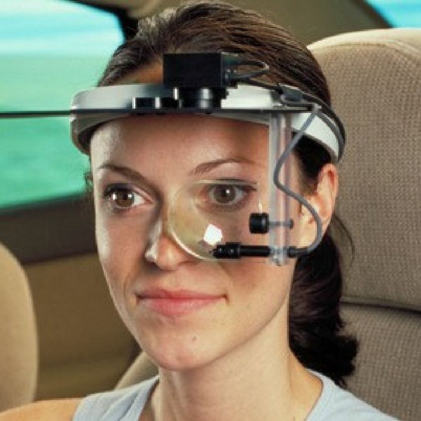
2

                                       Abstract

     Research indicates that monotonous automated driving increases the incidence of
fatigued driving. Although many prediction models based on advanced machine learning
techniques were proposed to monitor driver fatigue, especially in manual driving, little
is known about how these black-box machine learning models work. In this paper, we
proposed a combination of eXtreme Gradient Boosting (XGBoost) and SHAP (SHapley
Additive exPlanations) to predict driver fatigue with explanations due to their efficiency
and accuracy. First, in order to obtain the ground truth of driver fatigue, PERCLOS
(percentage of eyelid closure over the pupil over time) between 0 and 100 was used as
the response variable. Second, we built a driver fatigue regression model using both
physiological and behavioral measures with XGBoost and it outperformed other
selected machine learning models with 3.847 root-mean-squared error (RMSE), 1.768
mean absolute error (MAE) and 0.996 adjusted R2 . Third, we employed SHAP to
identify the most important predictor variables and uncovered the black-box XGBoost
model by showing the main effects of most important predictor variables globally and
explaining individual predictions locally. Such an explainable driver fatigue prediction
model offered insights into how to intervene in automated driving when necessary, such
as during the takeover transition period from automated driving to manual driving.
     Keywords: Driver fatigue prediction, explainability, automated driving,
physiological measures
3

                                     Introduction

     A driver may become fatigued or drowsy because of sleep deprivation, boredom, or
monotony, time-on-driving tasks, medication side-effects, or a combination of such
factors. Research indicates that the incidence of driver fatigue can be increased by
monotonous automated driving (Vogelpohl, Kühn, Hummel, & Vollrath, 2019). This
can be dangerous in SAE Level 2 - Level 4 (SAE, 2018) automated vehicles after the
driver is out of the control loop for prolonged periods (Hadi, Li, Wang, Yuan, & Cheng,
2020). Depending on the automation level of the vehicle, drivers need a high level of
situation awareness in SAE Level 2 (partial automation) automated vehicles and good
capabilities to respond to emerging hazards for takeover requests in SAE Level 3
(conditional automation) and Level 4 (high automation) automated vehicles (Collet &
Musicant, 2019). For example, takeover requests will be issued in conditional
automated driving, when the vehicle hits the operational limit, such as adverse weather
conditions and construction zones (Ayoub, Zhou, Bao, & Yang, 2019; Du, Zhou, et al.,
2020a, 2020b), which require the driver to safely take over control from automated
driving. Therefore, it is important to make sure that the driver is available and ready in
certain situations in automated driving (Du, Yang, & Zhou, 2020; Du, Zhou, et al.,
2020c; Zhou, Yang, & Zhang, 2019).
     Although driver fatigue has been widely studied in manual driving (e.g., see
(Dong, Hu, Uchimura, & Murayama, 2010; Sikander & Anwar, 2018)), the probe into
the fatigue prediction in automated driving seems limited. In automated driving, many
researchers instead focus on the influence of performing non-driving related tasks (e.g.,
cognitive workload, engagement, and distraction) on takeover performance (Clark,
McLaughlin, Williams, & Feng, 2017; Du, Zhou, et al., 2020a). On the other hand, if
drivers are not involved in non-driving related tasks, they would quickly show signs of
fatigue (Vogelpohl et al., 2019), which could potentially influence their takeover
performance, too. For example, Gonçalves, Happee, and Bengler (2016) found that
participants felt subjectively fatigued even after as short as 15 minutes of a monitoring
task in automated driving and Feldhütter, Gold, Schneider, and Bengler (2017)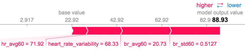
4

identified fatigue indicators among 31 participants in a 20-minute automated driving
scenario using eye-tracking data. Furthermore, in conditional automated driving, Hadi
et al. (2020) found that the higher the degree of fatigue was, the worse the takeover
performance. Hence, it is critical to detect and predict driver fatigue in monotonous
automated driving between SAE Level 2 and Level 4.
     Another phenomenon witnessed is that increasingly more researchers applied
advanced machine learning models in driver fatigue detection and prediction in order to
improve the performance of the models (see (Sikander & Anwar, 2018)) due to their
great successes in learning hidden patterns and making predictions of unobserved data,
such as deep learning models based on convolutional neural networks (CNNs) and long
short-term memory (LSTM). For example, Dwivedi, Biswaranjan, and Sethi (2014) used
CNNs to explicitly capture various latent facial features to detect driver drowsiness.
Nagabushanam, George, and Radha (2019) proposed a two-layer LSTM and four-layer
improved neural network deep learning algorithm for driver fatigue prediction and their
method outperformed other machine learning models.
     However, the trust and acceptance of such models can be compromised without
revealing the domain knowledge, i.e., explainability or interpretations, contained in the
data (Doshi-Velez & Kim, 2017). Unlike other domains, the importance of explainable
machine learning models in decision making with high risks is even greater, such as
medicine (Lundberg, Nair, et al., 2018) and transportation (Zhou et al., 2020). This is
also advocated by Mannering, Bhat, Shankar, and Abdel-Aty (2020) in safety analysis
to consider both predictability and causality using advanced machine learning model.
Furthermore, the domain knowledge captured by the machine learning models can be
further used as guidelines to address the issues at hand. For example, Caruana et al.
(2015) built a generalized additive model with pairwise interactions to predict
pneumonia risks and found that those with asthma were less likely to die from
pneumonia, which was counter-intuitive. However, by examining the data and the
model, the researchers found that those with asthma were intensively cared, which was
effective at reducing the likelihood of dying from pneumonia compared to the general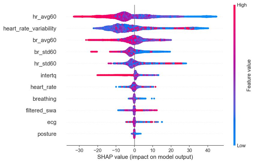
5

population. Such knowledge explained the model behavior. Thus, similar knowledge can
be potentially identified and used in driver fatigue prediction using explainable models
in manual and automated driving to help provide effective intervention measures.
     Towards this end, we proposed an explainable machine learning model to predict
driver fatigue using XGBoost (eXtreme Gradient Boosting) (Chen & Guestrin, 2016)
and SHAP (SHapley Additive exPlanations) (Lundberg et al., 2020; Lundberg, Nair, et
al., 2018) in automated driving. First, XGBoost is a highly effective and efficient
algorithm based on tree boosting and it is one of the most successful machine learning
algorithms in various areas, including driver fatigue prediction (Kumar, Kalia, &
Sharma, 2017). In order to understand the hidden patterns captured by the XGBoost
model, SHAP (Lundberg et al., 2020; Lundberg, Nair, et al., 2018) was used to explain
the XGBoost model by examining the main effects of the most important measures
globally and explaining individual prediction instances locally. SHAP uses the Shapley
value from cooperative game theory (Shapley, Kuhn, & Tucker, 1953) to calculate
individual contributions of the features in the prediction model and satisfies many
desirable properties in explaining machine learning models, including local accuracy,
missingness, and consistency (Lundberg et al., 2020). However, it is challenging to
compute the exact Shapley values for features of machine learning models, especially
deep learning models. Lundberg, Erion, and Lee (2018) proposed the SHAP algorithm
to reduce the complexity of calculating Shapley value in algorithms based on tree
ensembles from O(T L2M ) to O(T LD2 ), where T is the number of trees, L is the largest
number of leaves in the trees, M is the number of the features, and D is the maximum
depth of the trees. Hence, XGBoost and SHAP were used in this paper to predict driver
fatigue and uncover the hidden patterns in the machine learning model.

                                 RELATED WORK

Driver Fatigue Detection and Prediction

     Manual Driving. Driver fatigue has been studied widely in manual driving and
previous studies examined driver fatigue from two main types of measures, including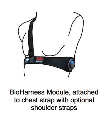
6

driving behavioral measures and physiological measures. Driving behavior measures
mainly include steering motion and lane deviation (Koesdwiady, Soua, Karray, &
Kamel, 2016). For example, Feng, Zhang, and Cheng (2009) found that driver fatigue
was negatively correlated with steering micro-corrections. Sayed and Eskandarian
(2001) proposed a fatigue prediction model with drivers’ steering angles based on an
artificial neural network that classified fatigued drivers and non-fatigued driver with
88% and 90% accuracy among 12 drivers. Using a sleep deprivation study (n = 12),
Krajewski, Sommer, Trutschel, Edwards, and Golz (2009) extracted features from slow
drifting and fast corrective counter steering to predict driver fatigue and their best
prediction accuracy was 86.1% in terms of classifying slight fatigue from strong fatigue.
Li, Chen, Peng, and Wu (2017) detected driver fatigue (n = 10) by calculating
approximate entropy features of steering wheel angles and yaw angles within a short
sliding window with 88.02% accuracy. McDonald, Lee, Schwarz, and Brown (2014)
applied a random forest steering algorithm to detect drowsiness indicated by lane
departure among 72 participants and it performed better than other algorithms (e.g.,
neural networks, SVMs, boosted trees). Though driving behavioral measures are easier
to collect, it is still challenging to obtain high prediction accuracy (McDonald et al.,
2014).
     Many studies investigated driver fatigue using physiological measures, which have
proven to be highly correlated with driver fatigue (Dong et al., 2010; Sikander &
Anwar, 2018). First, many researchers used head- and eye-related physiological data to
detect fatigue (Ji, Zhu, & Lan, 2004; Watta, Lakshmanan, & Hou, 2007). For instance,
Khan and Mansoor (2008) extracted features from the driver’ face and eyes to detect
driver fatigue (indicated by eye closure) with a normalized cross-correlation function,
which had 90% accuracy. PERCLOS (percentage of eyelid closure over the pupil over
time) and the average eye closure speed were used to detect driver fatigue using neural
networks (Chang & Chen, 2014). The system was able to detect fatigue with a success
rate of 97.8% among 4 participants. However, it dropped to 84.8% when the
participants wore glasses, and the reliability was susceptible to lighting, motion, and
7
occlusion (e.g., sunglasses). Second, other popular methods used measures derived from
EEG (electroencephalogram), EOG (electrooculography), ECG (electrocardiography),
and EMG (electromyography) for fatigue detection. For example, Jung, Shin, and
Chung (2014) examined heart rate variability to monitor driver fatigue. Zhang, Wang,
and Fu (2013) extracted entropy and complexity measures from EEG, EMG, and EOG
data of 20 subjects. Lee and Chung (2012) combined both photoplethysmography
(PPG) signals and facial features to detect driver fatigue (n = 10) and the model had a
true and false detection rate of 96% and 8%, respectively, using a dynamic Bayesian
network.
Automated Driving. Although these previous research endeavors provided
insights into the progression of driver fatigue in manual driving, limited research is
conducted in detecting and predicting driver fatigue in automated driving. Gonçalves et
al. (2016) found that participants were easily fatigued due to underload in automated
driving for 15 minutes of a monitoring task. Similarly, Feldhütter et al. (2017) found
fatigue signs due to underload in 31 participants using eye-tracking data for as short as
20-minute automated driving. Moreover, Körber, Cingel, Zimmermann, and Bengler
(2015) found that participants (n = 20) experienced substantial passive fatigue due to
monotony after 42 minutes of automated driving using eye-related data. Hadi et al.
(2020) demonstrated that drivers’ (n = 12) takeover performance was significantly worse
in various scenarios for fatigued driver in conditional automated driving. Vogelpohl et
al. (2019) (n = 60) indicated that compared to sleep-deprived drivers in manual driving,
drivers in automated driving exhibited facial indicators of fatigue 5 to 25 minutes earlier
and their takeover performance was significantly jeopardized. Therefore, fatigued
drivers could be one of the safety issues in takeover transition periods where a high level
of situation awareness is needed. These studies indicate the necessity for driver fatigue
detection and prediction in SAE Level 2 - Level 4 automated driving.8
Explainable Machine Learning Models
To detect and predict driver fatigue, it is extremely important to develop accurate
machine learning models in both manual driving and automated driving. For example,
CNN was used to extract spatial facial features in detecting driver fatigue (Dwivedi et
al., 2014) and LSTM was used to model temporal relations of physiological measures to
detect driver fatigue (Nagabushanam et al., 2019). Nevertheless, it can be difficult to
trust and accept such black-box models without revealing its domain knowledge
captured by the models, especially with the risks associated with the decisions based on
the models are high. Therefore, the choice between simple, easier to interpret models
and complex, black-box models is one of the important factors to consider in deploying
such models. Usually there are two types of explainable models, i.e., model-based and
post-hoc explainability (Murdoch, Singh, Kumbier, Abbasi-Asl, & Yu, 2019). Typical
examples of the model-based explainability include linear regression models, logistic
regression models, and single decision tree models. However, their performance is
usually inferior compared to complex black-box models. Post-hoc explainability is then
used to explain the behaviors and working mechanisms of black-box models
approximately, such as SHAP (Lundberg et al., 2020; Lundberg, Nair, et al., 2018) and
LIME (Local Interpretable Model-agnostic Explanations) (Ribeiro, Singh, & Guestrin,
2016). For example, LIME was used to explain neural network models in credit scoring
applications (Munkhdalai, Wang, Park, & Ryu, 2019) and SHAP was used to explain
ensemble machine learning models to identify risk factors during general anesthesia
(Lundberg, Nair, et al., 2018). Such explanation not only identified the key variables in
modeling, but also increased trust in real applications (Ayoub, Yang, & Zhou, 2021).
Compared to LIME, SHAP was better in explaining machine learning models in terms
of local accuracy and consistency (Lundberg et al., 2020).9
EXPERIMENT DESIGN
Participants
We excluded participants who had caffeine consumption, sleep disorders or other
factors that might have impacted driver fatigue. Finally, twenty participants were
recruited in this study (14 males and 6 females between 20 and 70 years old). In order
to elicit fatigue, unlike the common sleep deprivation method, we made use of the
nature of underload and monotony in automated driving to elicit passive fatigue in the
experiment in the afternoons. According to previous studies (Feldhütter et al., 2017;
Gonçalves et al., 2016; Körber et al., 2015), participants were expected to show passive
fatigue signs as soon as in 15 minutes without doing any secondary tasks and such
fatigue was more prevalent in automated driving.
Apparatus
The study took place in the VIRTTEX (VIRtual Test Track EXperiment) driving
simulator at Ford (see Figure 1b), a large six degree-of-freedom motion base simulator
that uses a hydraulically powered Stewart platform to reproduce vehicle motion. The
visual environment consists of a 240° front field-of-view and a 120° rear field-of-view.
Drivers were seated in a Ford Edge cab with 3D simulated sound to provide realistic
interior and exterior environment sounds, as well as a steering control loader for
accurate road feedback and tire forces to the driver. The simulator was configured with
an SAE Level 3 automated driving system and auditory-visual displays to indicate
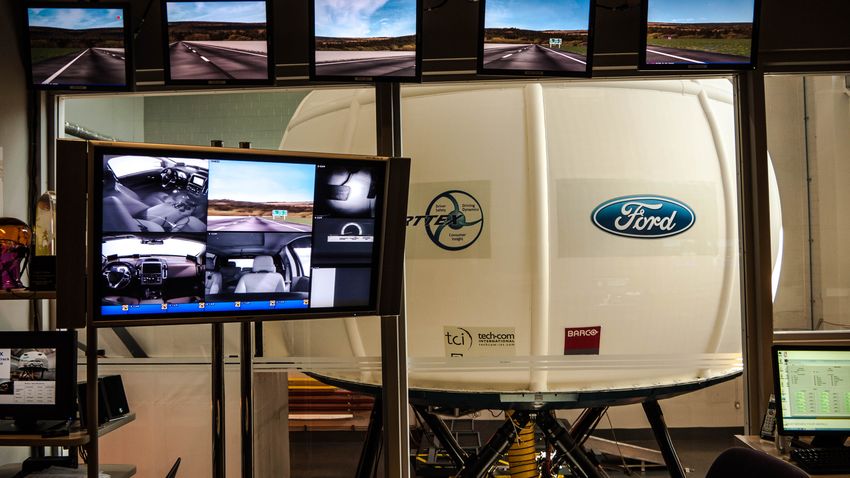
automated system status throughout the drive. The driver wore ISCAN© eye-tracking
goggles (ISCAN, Inc., MA, USA) outfitted with an eye camera, a dichroic mirror, and a
scene camera to track percent pupil occlusion in real time in order to calculate the
PERCLOS measure (see Figure 1c). Before entering the simulator, the participant was
outfitted with a BioHarness 3.0 Wireless Heart Rate Physiological Monitor (Zephyr
Technology, MD, USA) with Bluetooth to capture physiological measures (see Figure
1d).10
100
80
PERCLOS (%) 60
40
20
0
0 500 1000 1500 2000 2500 3000 3500
Time in Seconds
(a)
(b)
(c) (d)
Figure 1 . (a) Example PERCLOS time series data for a participant. (b) The
VIRTTEX driving simulator and driving scenarios with different views. (c) The
configuration of ISCAN Eye Tracker for PERCLOS measure collection. (d) BioHarness
model for physiological data collection.11
Simulator Scenario
The simulated drive was on a 4-lane undivided rural roadway with light traffic
flowing with and opposing the drivers. Drivers were instructed to initially stay in the
right lane and follow a lead vehicle that was varying its speed between 50 – 70 mph (80
– 115 kph). The driver then engaged the automated driving system using the steering
wheel controls. A key feature of this scenario was that, after the automation was
engaged for the data collection portion of the study, there were no secondary tasks at
all or no interaction with the research staff until the end of the session in order to elicit
passive driver fatigue in automated driving. There were also no hazardous events in the
automated driving session, which lasted about 60 minutes. With essentially no
disruptions, some drivers entered the fatigued state quickly (Feldhütter et al., 2017;
Gonçalves et al., 2016; Körber et al., 2015).
Predictor Variables and Response Variables
The response variable to be predicted was PERCLOS obtained from the ISCAN
eye tracker sampled at 60Hz. PERCLOS was operationally defined as the average
percent of the time the eyelids occluding the pupil (larger than 80%) using a 1-minute
moving window at any point in the data collection session during the experiment (Zhou
et al., 2020). A typical example of a fatigued participant was shown in Figure 1a.
The reason that we used PERCLOS as the ground truth of our prediction model
was that it was a reliable indicator of driver fatigue (Zhou et al., 2020), but it was
intrusive to measure in real applications (Figure 1 (c)). Therefore, we collected 11 less
intrusive measures as predictor variables as shown in Table 1 to predict driver fatigue
indicated by PERCLOS. A low pass filter was used to remove baseline wander noises in
ECG data (Kher, 2019). Breathing wave signals were filtered using a moving average
filter to remove noise. Steering wheel angles (swa), torque applied on steering wheel
(intertq), and posture data were also filtered by a low pass filter. Other measures, such
as hr_avg60, were then calculated based on the filtered signals.12
TABLE 1: Predictor variables used in modeling driver fatigue
Features Unit Explanation
heart_rate_variability millisecond (ms) Standard deviation of inter-beat interval
hr_avg60 beats/minute Average heart rate with a 60s sliding win-
dow
br_avg60 breaths/minute Average breathing rate with a 60s sliding
window
br_std60 breaths/minute Standard deviation of breathing rate with
a 60s sliding window
hr_std60 beats/minute Standard deviation of heart rate with a 60s
sliding window
heart rate beats/minute Number of beats in one minute
breathing bits Breathing waveform (16Hz)
ECG mV ECG waveform (250Hz)
intertq Nm Torque applied to steering wheel (200Hz)
swa degree Steering wheel angle (200Hz)
posture degree Degree from subject vertical (1Hz)
Experimental Procedure
Once participants had signed the informed consent form, they were given a brief
study introduction via a PowerPoint® presentation. The study introduction highlighted
the study objective to examine driver reactions to an automated driving system.
Participants were then given an overview of the automated driving system’s capabilities
and training on how to engage and disengage the system. Prior to entering the
VIRTTEX simulator, the participant donned the BioHarness 3.0 belt and Bluetooth
connectivity was verified. Once seated in the cab, the participant put on the
eye-tracking goggles. Up to 10 minutes was spent on calibrating the eye-tracker
(typically less than 5 minutes for drivers without glasses). Once the training was
complete, the participants transitioned right into the main drive. The driver was
instructed to engage the automation, monitor the driving task, and not to do any
secondary tasks or communicate with the experimenter.13
Driver Fatigue Prediction and Explanation
XGBoost
XGBoost is a highly efficient and effective machine learning model both for
regression and classification (Chen & Guestrin, 2016). In our driver fatigue prediction,
we used a one-second time window to discretize all the predictor variables, X = {xk },
and response variable, Y = {yk }, of all the participants, where k = 1, ..., n. The training
data set is indicated as D = {xk , yk , xk ∈ Rm , yk ∈ R}. In this research, n is the total
number of the samples and m is the number of the features (i.e., predictor variables),
and n = 58846, m = 11. Let ŷk denote the predicted result of a tree-based ensemble
model, ŷk = φ(xk ) = fs (xk ), where S is number of the trees in the regression
PS
s=1
model, fs xk is the s-th tree. For XGBoost, the objective function is regularized to
prevent over-fitting as follows:
X
L φ = l yk , ŷk + Ω fs , (1)
X
k s
where l is the loss function and in this research, we used root-mean-squared error
(RMSE). The penalty term Ω has the following form:
1
Ω fs ) = γT + λkwk2 , (2)
2
where γ and λ are the penalty parameters to control the number of leaves T and the
magnitude of leaf weights w. In the training process, XGBoost used an iterative process
to minimize the objective function and for the i-th step when adding a tree, fi , to the
model as follows:
X
(i−1)
Li φ = l yk , ŷk + fi (xk ) + Ω fi , (3)
k
This formula was approximated with a 2nd order Taylor expansion by substituting the
loss function with mean-squared error and after tree splitting from a given node, we14
have:
1 ( k∈KL gk )2 ( gk )2 gk )2
P P P
Lsplit = + P k∈KR − P k∈K − γ, (4)
2 ( k∈KL hk + λ) ( k∈KR hk + λ) ( k∈K hk + λ)
P
where K is a subset of observations for the given node and KL , KR are subsets of
observations in the left and right trees, respectively. gk and hk are the first and second
order gradient statistics on the loss function and are defined as
(j−1) (j−1)
gk = ∂ŷ(j−1) l yk , ŷk , hk = ∂ŷ2(j−1) l yk , ŷk . For a given tree structure, the
algorithm pushed gk and hk to the leaves they belong to, summed the statistics
together, and used Eq. (4) to identify the optimal splitting, which was similar to the
impurity measure in a decision tree, except that XGBoost also considered model
complexity in the training process.
SHAP
SHAP uses Shapley values (Shapley et al., 1953) based on coalitional game theory
to calculate individual contributions of each feature, which is named as SHAP values.
In this research, SHAP was used to explain the main effects in the XGBoost model and
individual predictions. According to (Lundberg et al., 2020; Lundberg, Nair, et al.,
2018), SHAP values are consistent and locally accurate individualized features that
obey the missingness property. The definition of the SHAP value of a feature-value set
is calculated for a model f below:
|S|!(m − |S| − 1)!
ϕi (v) = (fx (S ∪ {i}) − fx (S)), (5)
X
S⊆N \{i}
m!
where fx (S) = E[f (x)|xS ] is the contribution of coalition S in predicting driver fatigue,
indicated by PERCLOS in this study, S is a subset of the input features, N is the set of
all the input features, and m = 11 is the total number of features. The summation
extends over all subsets S of N that does not contain feature i. However, it is
challenging to estimate the value of fx (S) efficiently due to the exponential complexity
in Eq. (5). Lundberg, Nair, et al. (2018) proposed an algorithm to approximate the15
values of E[f (x)|xS ] for tree-based models, such as XGBoost, in O(T LD2 ) time, where
T is the number of the trees, L is the number of maximum leaves in any tree, and
D = logL. SHAP uses the difference between individual fatigue prediction against the
average fatigue prediction, which is fairly distributed among all the feature-value sets in
the data (see Figure 5). Hence, it has a solid theory foundation in explaining our
XGBoost model.
Results
Prediction Results by XGBoost
First, we compared the performance of the XGBoost prediction model with other
six regression models, including linear regression, linear SVM, quadratic SVM, Gaussian
SVM, decision trees, random forest. The setting of the XGBoost was as follows: max
depth = 10, learning rate = 0.1, objective = reg:squarederror, number of estimators =
150, regularization parameter alpha = 1, subsample = 0.9, and colsample = 0.9. All the
11 predictor variables were included in all the models with 10-fold cross validation,
except the last entry for XGBoost (best), where only 5 most important features were
selected to obtain the best performance (see Figure 3). We reported the results in
predicting PERCLOS (0-100) with the following three performance metrics, including
RMSE (the smaller the better), MAE (i.e., mean absolute error, the smaller the better),
and adjusted R2 (the closer to 1, the better) defined as follows:
v 2
uP
u n − ŷk
t k=1 yk
RM SE = , (6)
n
Pn
|yk − ŷk |
M AE = k=1
, (7)
n
n−1
Adj. R2 = 1 − (1 − R2 ) , (8)
n−m−116
where n is the total number of the samples, ŷ is the predicted value of the ground
k
Pn 2
SSregression ŷk −y
truth, yk , and R2 = =P 2 , and m is the total number of the
k=1
SStotal n
k=1
yk −y
predictor variables. The results are shown in Table 2. It can be seen that XGBoost
outperformed other machine learning models.
TABLE 2: Comparisons of prediction results of different machine
learning models
Model RMSE MAE Adj. R2
Linear Regression 26.429 20.189 0.250
Linear SVM 28.972 18.793 0.102
Quadratic SVM 25.995 16.537 0.269
Gaussian SVM 18.027 11.915 0.653
Fine Tree 6.753 2.516 0.951
Random Forest 6.700 3.910 0.950
XGBoost (all) 4.788 2.316 0.993
XGBoost (best) 3.847 1.768 0.996
Note XGBoost (all) indicates all the 11 predictors were included in the model and
XGBoost (best) indicate only five of the most important features were included (see
Figure 3).
SHAP Explanation
Feature Importance. During the 10-fold cross-validation process, we used the
test data in each fold to calculate the SHAP values in order to improve its
generalizability so that each sample was calculated its SHAP value for exactly once. We
used the SHAP values in Eq. 5 to identify the most important features as shown in
Figure 2. The feature importance was sorted by their global impact k | identified
Pn
k=1 |ϕm
by SHAP plotted vertically as follows: hr_avg60 is the most important, followed by
heart_rate_variability, br_avg60, br_std60, hr_std60, and so on. Every sample in the
data was run through the model and each dot (i.e., ϕm
k ) was created for each feature
value and was plotted horizontally. The more important the feature is, the more impact
on the model output. For example, hr_avg60 had a range of SHAP value (i.e.,
PERCLOS) between -40 and 60. Note that the SHAP value was computed with regard
to the base average output (see Figure 5) and hr_avg60 could push some extreme
output 40 lower than the average and push some other extreme output 60 higher than17
the average. It tended to show that the higher the value of hr_avg60, the lower the
predicted PERCLOS.
Figure 2 . Importance ranking of 11 features identified by SHAP summary plot. The
higher the SHAP value of a feature, the higher the predicted PERCLOS.
Prediction Results with an Optimal Subset of Features. We further
added one feature at a time to the XGBoost model starting from the most important
identified as shown in Figure 2. Figure 3 shows that the performance was increasing
when more features were added until when there were 5 features (i.e., hr_avg60,
heart_rate_variability, br_avg60, br_std60, and hr_std60) in the prediction model.
The performance was better than that obtained by the model when 11 predictors were
included, i.e., a subset of important features had the optimal performance (see Table 2).
Main Effects. We also examined the main effects of the top five most
important features when the model had the best performance in Figure 3. Figure 4
shows the main effects. Consistent with Figure 2, the overall trend is that the larger the
value of hr_avg60, the smaller the SHAP values (i.e., predicted PERCLOS), but not in
an exact linear fashion (see Figure 4c). The slope is much larger in a narrow interval
around 50 and 55 beats/min than others and between 55 and 63 beats/min, it is almost18
(a) (b)
Figure 3 . How performance changes when the model added one feature at a time from
the most important one to the least important one: (a) RMSE and MAE; (b) Adjusted
R2 . Note the error bar was the standard deviation obtained in the ten-fold cross
validation process.
flat. When it is larger than 63 beats/min, the larger the value of hr_avg60, the smaller
the predicted PERCLOS. For heart_rate_variability, it has a V-shape relationship with
the predicted PERCLOS (see Figure 4b). The predicted PERCLOS is decreasing when
the value of heart_rate_variability is smaller than about 50 ms while the predicted
PERCLOS is increasing when it is going up from 50 ms to 140ms. The overall trend for
br_avg60 is that the larger the value of br_avg60, the smaller the predicted
PERCLOS, and this trend was not obvious until the value of br_avg60 is larger than 15
breaths/min (see Figure 4c). The overall trend for br_std60 is that the predicted
PERCLOS is decreasing when the value of br_std60 is increasing until it reaches
around 0.8 breaths/min, after which the predicted PERCLOS seems flat (see Figure
4d). The predicted PERCLOS decreases when the value of br_avg60 increases from 1
beat/min to 2 beats/min. Then the trend tends to be reversed, i.e., the larger the value
of br_avg60, the larger the value of the predicted PERCLOS (see Figure 4e). Note the
importance or the global impact of each individual feature is also noticeable in the
range of predicted PERCLOS, where hr_avg60 has the maximum range, followed by
heart_rate_variability, while the rest have similar ranges.19
(a)
(b) (c)
(d) (e)
Figure 4 . Main effects of the most important features. (a) hr_avg60; (b)
heart_rate_variability; (c) br_avg60; (d) br_std60; (e) hr_std60. Note only data
between the 2.5th percentile and the 97.5th percentile were included in the figures.20
(a)
(b)
Figure 5 . SHAP individual explanations. (a) An example of low predicted driver
fatigue; (b) An example of high predicted driver fatigue. Note the base value, 22.92,
indicated the average predicted PERCLOS by all the training data in the model and
those in blue push the predicted value lower and those in red push the predicted value
higher.
Individual Explanations. SHAP is also able to produce individual
explanations locally to show the contributions of each input feature. Figure 5 shows two
examples. The base value is the averaged output from the model, which was 22.92, the
feature-value sets in blue push the output (predicted PERCLOS) lower, and the
feature-value sets in red push the output higher. For example, the feature-value sets in
Figure 5a push the output value to be 25.90, which was very close to the ground-truth
value at 26.16. hr_avg60 and br_std60 push the predicted PERCLOS higher while
br_avg60, heart_rate_variability push the predicted PERCLOS lower. The feature
hr_avg60 contributes the most to such an output. All the feature-value sets in Figure
5b push the output higher to be 88.93, which was also close to the ground true value at
90.91. Among them, br_std60 contributes the most, followed by br_avg60,
heart_rate_variability, and hr_avg60. Therefore, despite the fact that globally
hr_avg60 is the most important feature, its contribution might not always be the
largest locally.21
Discussions
Fatigue Prediction
The proposed model used both physiological and behavioral measures to predict
driver fatigue indicated by the PERCLOS measure. The model used 11 predictor
variables as input and the model with best performance only made use of heart data
and breathing data and was able to predict driver fatigue with high accuracy in real
time. With Python 3.8 on a MacBook Pro with 2.3GHz Quad-Core Intel Core i7 and
macOS Catalina, the average prediction time for one sample was only 3.6 × 10⁻⁶
seconds. Compared with the fatigue-related studies in automated driving, our work
used prediction models rather than simply described the fatigue progression in
automated driving. Moreover, we identified the most important features in predicting
driver fatigue in automated driving using SHAP, including hr_avg60,
heart_rate_variability, br_avg60, br_std60, and hr_std60. Therefore, the included
physiological measures were found to be more important than the included behavioral
measures. The prediction model provided one good way to monitor, quantify, detect,
and predict driver fatigue in real time. Despite the fact that fatigue has many
components in terms of its bodily representation, multiple physiological measures were
able to predict driver fatigue with RMSE = 3.847, MAE = 1.768, and adjusted
R2 = 0.996. During automated driving, wearable physiological sensors can be
potentially used to detect and predict drivers’ fatigued state in real time in a minimally
invasive manner. Such insights give us informed design guidelines in customizing driver
fatigue models by tuning only the most critical physiological measures.
Model Explanation
Unlike previous driver fatigue prediction studies, the most important findings in
this study are the relationships between the five most important measures identified by
SHAP and driver fatigue indicated by PERCLOS. For example, hr_avg60 and
br_avg60 tended to be negatively correlated with predicted driver fatigue except at
some specific, narrow intervals (see Figures 4a and 4c). This could be caused by the22
individual differences or noises involved in the dataset. However, such domain
knowledge captured in the driver fatigue prediction model can be used to help design
systems that fight driver fatigue in automated driving.
First, consistent with previous studies (e.g., (Ünal, de Waard, Epstude, & Steg,
2013)), a low heart rate can be indicative of a low level of arousal with low vigilance. In
order to fight monotony in automated driving, music with high tempos, for example, can
be used to increase drivers’ heart rate to help drivers stay at an optimal level of arousal
to improve driving performance (Dalton, Behm, & Kibele, 2007). Compared to a
control group with no music, participants with self-selected music increased 3 beats/min
on average, which could decrease PERCLOS by as much as 40 (see Figure 4a). Second,
consistent with previous studies (e.g., (Sun, Yu, Berilla, Liu, & Wu, 2011)), a decreasing
breathing rate was also a sign of the onset of fatigue. To fight monotonous driver fatigue
in automated driving, a breath booster system based on haptic guidance was proposed
to increase breathing rate and heart rate in order to increase driver alertness and focus
(Balters, Murnane, Landay, & Paredes, 2018). However, what is less known is that a
smaller br_std60 was also associated with driver fatigue. A variable breath pattern
could also be used to fight driver fatigue. Third, heart_rate_variability was computed
as the standard deviation of inter-beat intervals while hr_std60 was calculated as the
standard deviation of heart rate (see Table 1). In addition, both had a V-shape
relationship with the predicted PERCLOS (see Figures 4b and 4e). In this sense, they
described the same heart rate activity and its association with driver fatigue. Increases
in heart_rate_variability could be associated with decreases in mental workload, which
often occurred in sleepy drivers with monotonous driving (Horne & Reyner, 1995). This
was consistent with our finding when heart_rate_variability was between 50 and 140
ms or when hr_std60 was between 2 beats/min and 8 beats/min (see Figures 4b and
4e). However, in other intervals, increases in heart_rate_variability led to decreases in
driver fatigue, especially when it was smaller than 50 ms or hr_std60 was smaller than
2 beats/min. This was not reported previously and could be potentially explained by
the different measures used for heart rate variability. For example, Fujiwara et al.23
(2018) specifically included a feature named NN50, which was defined as the number of
adjacent inter-beat intervals whose difference was more than 50 ms within a period of
time. This is consistent with our results, where 50 ms was the turning point in the
V-shape relationship between heart_rate_variability and the predicted PERCLOS.
Limitations and Future Work
First, we used XGBoost to predict driver fatigue without considering the temporal
relationships among the training data. A model, such as LSTM, can potentially
improve the performance of the model further by examining the temporal relationships
in the data in the future. However, the cost of better performance of LSTM is that it
would be difficult to explain the captured knowledge by LSTM using SHAP. Moreover,
it might still be not adequate to detect and predict driver fatigue in real time and more
research should be devoted to predicting driver fatigue ahead of time in order for the
driver to prepare possible hazards in the takeover process in automated driving (Zhou
et al., 2020). Second, it should be cautious to generalize our results to other situations
because driver fatigue in this study mainly refers to passive fatigue due to monotonous
automated driving, which can be different from fatigue caused by sleep-deprivation in
traditional manual driving. In this sense, our model is more appropriate for fatigue
monitoring in automated driving rather than in manual driving.
Conclusion
In this study, we built a fatigue prediction model using XGBoost in automated
driving. In order to understand the black-box XGBoost model, we utilized SHAP based
on coalitional game theory. First, SHAP was used to identify the most important
measures among the 11 predictor variables and using only the top five most important
predictor variables, the XGBoost was able to predict driver fatigue indicated by
PERCLOS accurately. Second, SHAP was able to identify the main effects of the
important predictor variables in the XGBoost model globally. Third, SHAP also offered
individual prediction explanations to understand the contributions of each predictor
variable locally. These insights can potentially help automotive manufacturers design24 more acceptable and trustworthy fatigue detection and prediction models in automated vehicles.
25

                                      References

Ayoub, J., Yang, X. J., & Zhou, F. (2021). Modeling dispositional and initial learned
     trust in automated vehicles with predictability and explainability. Transportation
     Research Part F: Traffic Psychology and Behaviour, 77 , 102 - 116.
Ayoub, J., Zhou, F., Bao, S., & Yang, X. J. (2019). From manual driving to automated
     driving: A review of 10 years of autoui. In Proceedings of the 11th international
     conference on automotive user interfaces and interactive vehicular applications
     (pp. 70–90).
Balters, S., Murnane, E. L., Landay, J. A., & Paredes, P. E. (2018). Breath booster!
     exploring in-car, fast-paced breathing interventions to enhance driver arousal
     state. In Proceedings of the 12th eai international conference on pervasive
     computing technologies for healthcare (pp. 128–137).
Caruana, R., Lou, Y., Gehrke, J., Koch, P., Sturm, M., & Elhadad, N. (2015).
     Intelligible models for healthcare: Predicting pneumonia risk and hospital 30-day
     readmission. In Proceedings of the 21th acm sigkdd international conference on
     knowledge discovery and data mining (pp. 1721–1730).
Chang, T.-H., & Chen, Y.-R. (2014). Driver fatigue surveillance via eye detection. In
     17th international ieee conference on intelligent transportation systems (itsc) (pp.
     366–371).
Chen, T., & Guestrin, C. (2016). Xgboost: A scalable tree boosting system. In
     Proceedings of the 22nd acm sigkdd international conference on knowledge
     discovery and data mining (pp. 785–794).
Clark, H., McLaughlin, A. C., Williams, B., & Feng, J. (2017). Performance in takeover
     and characteristics of non-driving related tasks during highly automated driving
     in younger and older drivers. In Proceedings of the human factors and ergonomics
     society annual meeting (Vol. 61, pp. 37–41).
Collet, C., & Musicant, O. (2019). Associating vehicles automation with drivers
     functional state assessment systems: A challenge for road safety in the future.
     Frontiers in human neuroscience, 13 , 131.
26
Dalton, B. H., Behm, D. G., & Kibele, A. (2007). Effects of sound types and volumes
on simulated driving, vigilance tasks and heart rate. Occupational Ergonomics,
7 (3), 153–168.
Dong, Y., Hu, Z., Uchimura, K., & Murayama, N. (2010). Driver inattention
monitoring system for intelligent vehicles: A review. IEEE transactions on
intelligent transportation systems, 12 (2), 596–614.
Doshi-Velez, F., & Kim, B. (2017). Towards a rigorous science of interpretable machine
learning. arXiv preprint arXiv:1702.08608 .
Du, N., Yang, X. J., & Zhou, F. (2020). Psychophysiological responses to takeover
requests in conditionally automated driving. Accident Analysis & Prevention,
148 , 105804.
Du, N., Zhou, F., Pulver, E., Tilbury, D., Robert, L. P., Pradhan, A. K., & Yang, X. J.
(2020c). Predicting takeover performance in conditionally automated driving. In
Extended abstracts of the 2020 chi conference on human factors in computing
systems (pp. 1–8).
Du, N., Zhou, F., Pulver, E. M., Tilbury, D. M., Robert, L. P., Pradhan, A. K., &
Yang, X. J. (2020a). Examining the effects of emotional valence and arousal on
takeover performance in conditionally automated driving. Transportation research
part C: emerging technologies, 112 , 78–87.
Du, N., Zhou, F., Pulver, E. M., Tilbury, D. M., Robert, L. P., Pradhan, A. K., &
Yang, X. J. (2020b). Predicting driver takeover performance in conditionally
automated driving. Accident Analysis & Prevention, 148 , 105748.
Dwivedi, K., Biswaranjan, K., & Sethi, A. (2014). Drowsy driver detection using
representation learning. In 2014 ieee international advance computing conference
(iacc) (pp. 995–999).
Feldhütter, A., Gold, C., Schneider, S., & Bengler, K. (2017). How the duration of
automated driving influences take-over performance and gaze behavior. In
Advances in ergonomic design of systems, products and processes (pp. 309–318).
Springer.27
Feng, R., Zhang, G., & Cheng, B. (2009). An on-board system for detecting driver
drowsiness based on multi-sensor data fusion using dempster-shafer theory. In
2009 international conference on networking, sensing and control (pp. 897–902).
Fujiwara, K., Abe, E., Kamata, K., Nakayama, C., Suzuki, Y., Yamakawa, T., . . .
others (2018). Heart rate variability-based driver drowsiness detection and its
validation with eeg. IEEE Transactions on Biomedical Engineering, 66 (6),
1769–1778.
Gonçalves, J., Happee, R., & Bengler, K. (2016). Drowsiness in conditional automation:
proneness, diagnosis and driving performance effects. In 2016 ieee 19th
international conference on intelligent transportation systems (itsc) (pp. 873–878).
Hadi, A. M., Li, Q., Wang, W., Yuan, Q., & Cheng, B. (2020). Influence of passive
fatigue and take-over request lead time on drivers’ take-over performance. In
International conference on applied human factors and ergonomics (pp. 253–259).
Horne, J. A., & Reyner, L. A. (1995). Sleep related vehicle accidents. Bmj, 310 (6979),
565–567.
Ji, Q., Zhu, Z., & Lan, P. (2004). Real-time nonintrusive monitoring and prediction of
driver fatigue. IEEE transactions on vehicular technology, 53 (4), 1052–1068.
Jung, S.-J., Shin, H.-S., & Chung, W.-Y. (2014). Driver fatigue and drowsiness
monitoring system with embedded electrocardiogram sensor on steering wheel.
IET Intelligent Transport Systems, 8 (1), 43–50.
Khan, M. I., & Mansoor, A. B. (2008). Real time eyes tracking and classification for
driver fatigue detection. In International conference image analysis and
recognition (pp. 729–738).
Kher, R. (2019). Signal processing techniques for removing noise from ecg signals. J.
Biomed. Eng. Res, 3 , 1–9.
Koesdwiady, A., Soua, R., Karray, F., & Kamel, M. S. (2016). Recent trends in driver
safety monitoring systems: State of the art and challenges. IEEE transactions on
vehicular technology, 66 (6), 4550–4563.28
Körber, M., Cingel, A., Zimmermann, M., & Bengler, K. (2015). Vigilance decrement
and passive fatigue caused by monotony in automated driving. Procedia
Manufacturing, 3 , 2403–2409.
Krajewski, J., Sommer, D., Trutschel, U., Edwards, D., & Golz, M. (2009). Steering
wheel behavior based estimation of fatigue. In Proceedings of the... international
driving symposium on human factors in driver assessment, training and vehicle
design (Vol. 5, pp. 118–124).
Kumar, S., Kalia, A., & Sharma, A. (2017). Predictive analysis of alertness related
features for driver drowsiness detection. In International conference on intelligent
systems design and applications (pp. 368–377).
Lee, B.-G., & Chung, W.-Y. (2012). Driver alertness monitoring using fusion of facial
features and bio-signals. IEEE Sensors Journal, 12 (7), 2416–2422.
Li, Z., Chen, L., Peng, J., & Wu, Y. (2017). Automatic detection of driver fatigue using
driving operation information for transportation safety. Sensors, 17 (6), 1212.
Lundberg, S. M., Erion, G., Chen, H., DeGrave, A., Prutkin, J. M., Nair, B., . . . Lee,
S.-I. (2020). From local explanations to global understanding with explainable ai
for trees. Nature machine intelligence, 2 (1), 2522–5839.
Lundberg, S. M., Erion, G. G., & Lee, S.-I. (2018). Consistent individualized feature
attribution for tree ensembles. arXiv preprint arXiv:1802.03888 .
Lundberg, S. M., Nair, B., Vavilala, M. S., Horibe, M., Eisses, M. J., Adams, T., . . .
others (2018). Explainable machine-learning predictions for the prevention of
hypoxaemia during surgery. Nature biomedical engineering, 2 (10), 749–760.
Mannering, F., Bhat, C. R., Shankar, V., & Abdel-Aty, M. (2020). Big data, traditional
data and the tradeoffs between prediction and causality in highway-safety
analysis. Analytic methods in accident research, 25 , 100113.
McDonald, A. D., Lee, J. D., Schwarz, C., & Brown, T. L. (2014). Steering in a random
forest: Ensemble learning for detecting drowsiness-related lane departures.
Human factors, 56 (5), 986–998.
Munkhdalai, L., Wang, L., Park, H. W., & Ryu, K. H. (2019). Advanced neural29
network approach, its explanation with lime for credit scoring application. In
Asian conference on intelligent information and database systems (pp. 407–419).
Murdoch, W. J., Singh, C., Kumbier, K., Abbasi-Asl, R., & Yu, B. (2019). Definitions,
methods, and applications in interpretable machine learning. Proceedings of the
National Academy of Sciences, 116 (44), 22071–22080.
Nagabushanam, P., George, S. T., & Radha, S. (2019). Eeg signal classification using
lstm and improved neural network algorithms. Soft Computing, 1–23.
Ribeiro, M. T., Singh, S., & Guestrin, C. (2016). " why should i trust you?" explaining
the predictions of any classifier. In Proceedings of the 22nd acm sigkdd
international conference on knowledge discovery and data mining (pp. 1135–1144).
SAE. (2018). Taxonomy and definitions for terms related to driving automation systems
for on-road motor vehicles. SAE International in United States, J3016–201806.
Sayed, R., & Eskandarian, A. (2001). Unobtrusive drowsiness detection by neural
network learning of driver steering. Proceedings of the Institution of Mechanical
Engineers, Part D: Journal of Automobile Engineering, 215 (9), 969–975.
Shapley, L. S., Kuhn, H., & Tucker, A. (1953). Contributions to the theory of games.
Annals of mathematics studies, 28 (2), 307–317.
Sikander, G., & Anwar, S. (2018). Driver fatigue detection systems: A review. IEEE
Transactions on Intelligent Transportation Systems, 20 (6), 2339–2352.
Sun, Y., Yu, X., Berilla, J., Liu, Z., & Wu, G. (2011). An in-vehicle physiological signal
monitoring system for driver fatigue detection. In 3rd international conference on
road safety and simulationpurdue universitytransportation research board.
Ünal, A. B., de Waard, D., Epstude, K., & Steg, L. (2013). Driving with music: Effects
on arousal and performance. Transportation research part F: traffic psychology
and behaviour, 21 , 52–65.
Vogelpohl, T., Kühn, M., Hummel, T., & Vollrath, M. (2019). Asleep at the automated
wheel—sleepiness and fatigue during highly automated driving. Accident Analysis
& Prevention, 126 , 70–84.30
Watta, P., Lakshmanan, S., & Hou, Y. (2007). Nonparametric approaches for
estimating driver pose. IEEE transactions on vehicular technology, 56 (4),
2028–2041.
Zhang, C., Wang, H., & Fu, R. (2013). Automated detection of driver fatigue based on
entropy and complexity measures. IEEE Transactions on Intelligent
Transportation Systems, 15 (1), 168–177.
Zhou, F., Alsaid, A., Blommer, M., Curry, R., Swaminathan, R., Kochhar, D., . . . Lei,
B. (2020). Driver fatigue transition prediction in highly automated driving using
physiological features. Expert Systems with Applications, 113204.
Zhou, F., Yang, X. J., & Zhang, X. (2019). Takeover transition in autonomous vehicles:
A You Tube study. International Journal of Human–Computer Interaction, 1–12.You can also read