Predicting Home Value in California, United States via Machine Learning Modeling
←
→
Page content transcription
If your browser does not render page correctly, please read the page content below
STATISTICS, OPTIMIZATION AND INFORMATION COMPUTING
         Stat., Optim. Inf. Comput., Vol. 7, March 2019, pp 66–74.
         Published online in International Academic Press (www.IAPress.org)

  Predicting Home Value in California, United States via Machine Learning
                                Modeling

                                                        Yitong Huang
                               Department of Computer Science, Illinois Institute of Technology, USA

Abstract The market value of real estate is difficult to predict with simple regression model due to the diversity and
complexity of the real data. In this paper, with the latest real estate data of three counties in Los Angeles, California, United
States, both linear and non-linear machine learning methods are employed to predict the log error of the home value. The
motivation is to improve the accuracy in home value prediction with advanced methods. The main contribution is that it finds
that traditional linear models are not predictive for complex home value data sets, while tree based non-linear models are
most accurate with the lowest mean square errors.

Keywords home value; log error, linear regression; decision tree; boosting; random forest; SVM

AMS 2010 subject classifications 62J05
DOI: 10.19139/soic.v7i1.435

1. Introduction

A group of remarkable and provident pioneers set forth from Dartmouth College in the summer of 1956 and started
the study of artificial intelligence (AI)[1, 2]. At first, the focus was on theoretical models. However, the interest and
funding finally drained off. In the winter of AI, people never stopped thinking about the question whether a machine
can think. As the developing of technology, and the emergence of large numbers of successful incidents of AI,
people discovered the unreasonable effectiveness of data[3]. Unlike the standstill of the theoretical studies, people
started to teach the machine to learn[4, 5, 6]. In particular, a machine is said to learn when it changes its behavior
based on experience, which in most cases is the data. Without a specific model, such as the various neat physics
formulas, we teach the machine to learn from the data directly. To some extent, AI was born to mimic human,
but when it comes to human, stories become complex, especially for decision making[7, 8, 9]. Home, as the most
important part of a person, and one of the most expensive consumption (or investment) in one’s life, undoubtedly
worth a serious decision. Whether a machine can learn some aspects of such a decision-making process based on
adequate information really attracts us. Zillow, founded in 2006, together with Yahoo Real Estate, create one of
the largest real estate advertising networks[10, 11, 12]. Fortunately, Zillow is seeking help on improving home
value estimations and is willing to share adequate real data. This paper proposes to analyze home value based
on a full list of real estate properties in three counties -Los Angeles, Orange and Ventura in California USA in 2016.

Roy E. Lowrance[13] developed a linear model of residential real estate prices for 2003 through 2009 in
Los Angeles County. He tested designs for linear models to determine the best form for the model as well as the
training period, features, and regularizer that produce the lowest errors. And he compared the best of linear models

∗ Correspondence to: Yitong Huang (Email: yhuang109@hawk.iit.edu Alternative Email: hopeyitong@gmail.com). Department of
Computer Science, Illinois Institute of Technology, Chicago, IL 60616, USA.

ISSN 2310-5070 (online) ISSN 2311-004X (print)
Copyright ⃝
          c 2019 International Academic Press
Y. HUANG                                                         67

to random forests, the result showed that the random forests model, with minimal design work, outperformed the
carefully designed local linear model. Hu et al.[14] built multivariate regression models of home prices using a
dataset composed of 81 homes. They applied the maximum information coefficient MIC) statistics to observed
home values and predicted ones as the evaluation method, and found high strength of the relationship between
observer and predictor. Vapnik[15] introduced three kinds of a support vector machine (SVM) such as a hard
margin SVM (H-SVM), a soft margin SVM (S-SVM) and a kernel SVM. Statistical users accept SVM examined
by the real data[16]. Due to high nonlinearity of the house value data, Mu et al[17]. used support vector machine
(SVM), least squares support vector machine (LSSVM) and partial least squares (PLS) to forecast the values
of Boston suburb houses. They found SVM and LSSVM are superior to PLS on dealing with the problem of
nonlinearity, and the best performance can be achieved by SVM because of solving quadratic programming
problem. All these previous work clearly indicates that non-linear models would be much better than linear
regression for house value prediction.

This paper uses the data set containing all the transactions before October 15, 2016, plus some of the
transactions after October 15, 2016. 58 features are given for each home, including from the count of the bedrooms
and bathrooms, to the count of the pools. In short, all the home related features are provided, although some of
the features contain a large number of missing values. The major goal is to predict the error between Zestimate
and actual sale price. Where Zestimate home value is Zillow’s estimated market value for an individual home
and is calculated for about 100 million homes nationwide. It is a starting point in determining a home’s value
and is not an official appraisal. The Zestimate is automatically computed daily based on millions of public and
user-submitted data points. This paper will compare the prediction results across a variety of methods and the
measure is MSE. The objective is to predict the home value based on the various home features. The data provides
as many as 59 properties including built of year, total area, number or bedrooms and so on. This paper will pick
the important features and apply machine learning models to predict the sale price of the real estate.

2. Methods

Figure 1 plotted the percentage of missing data for each feature, which is a very important baseline when choosing
features. In general, the features are classified into three parts: conditions of the estate, such as bathroom count
and bedroom count; the facilities, including the pool count; location. Some features containing more than 80%
of missing value are still maintained when they are explained reasonable enough. For example, although 80.2%
of pool counts are missing, we may interpret as there is no pool and fill NA with 0. After refinement, there are
28 features left. The left features in condition of the estate are: bathroom count, bedroom count, ? bathroom
count, calculated finished sqf, unit count, year build, total tax assessed value, assessed value of the built structure,
assessed value of the land area, tax amount; the left features in facility are: air conditioning type, building quality
type, federal information, garage count, garage total sqf, heating sys type, parking lot sqf, number of stories, pool
count; the left features in location are: latitude, longitude, property land use type, county id, zip. In addition, the
transaction date is converted to the days from the beginning of the year 01/01/2016, adding as another feature.

After the first step of cleaning, there are 89412 rows of data, 30 columns, which is referred to later as the
preprocessed dataset. One of the column is logerror, our model response, which is defined as

log(error) = log(Zestimate) − log(SaleP rice)

The goal is to predict the logerror based on all the other features. The full data set is separated into two
subsets, train and test. In particular, half of the data is selected as train set and the other half as the test set.
The models are trained using the same train set and test on the same test set for all methods. The task is really
competitive. As Zestimate gives a rather accurate estimation to the real sale price, which leads to a very small
logerror in most cases. This makes prediction task really competitive. In fact, classic linear regression and

                                                                             Stat., Optim. Inf. Comput. Vol. 7, March 2019
68 PREDICTING HOME VALUE IN CALIFORNIA, UNITED STATES VIA MACHINE LEARNING MODELING
Figure 1. Percentage of missing data of each feature.
regression tree gives no results at all: the adjusted R-square is tiny (less than 0.1) for linear regression, while the
regression tree results in a single node. Upon this fact, the results are experimented and compared among linear
regression model and other non-linear models. Since in the common sense, location, bedroom count, total area,
are usually considered as the most important features of an estate. The large logerror (logerror>2) map with the
real latitude and longitude are given in Figure 2.
This concludes the preparation of the data. However, for linear regression, tree based method and boosting,
less features are preferred to improve the interpretability. So some features are deleted later on. This smaller data
set will be referred to as post-processed data set. However, the experiments show that deleting features by intuition
is not a good idea. This will be further explained later. Linear regression, and some non-linear models such as
decision tree, boosting, random forest and SVM are used to predict the home value. The results are given in next
section.
3. Results and discussion
3.1. Linear Regression
First, linear regression is run on all the features with all the preprocessed data. The adjusted R-square is 0.006,
which means there is almost no linearity for the dataset and linear regression is not a valid model in this case.
However, the MSE is very small as 0.026. Second, we include all the possible interactions in linear regression.
The adjusted R-square is 0.03 in this case. Third, in order to improve interpretability, we further processed the
data. According to some previous related work and life experience, some features like firelaceflag that barely
have relationship with housing price were deleted. To do further future selection, random forest is run to see the
importance of each feature variables, and the results are shown in Table 1. After deleting unimportant features,
there are 16 predictors left (parcelid not included). Now the new data frame has dimension 24156 x 18. This will
Stat., Optim. Inf. Comput. Vol. 7, March 2019Y. HUANG 69
Figure 2. Log error map with real latitude and longitude.
be referred to as post-processed dataset.
To make sure that the left features are somewhat important, Lasso regression is processed based on the
new data frame. Results show that there are no 0 coefficients. So all features are kept to do following regression
approach. This result indicates that too many data are deleted. The data is scaled. It results in a very low adjusted
r-square value, which is 0.007005. The result here is not surprising, since almost none of previous related work get
a good result with linear regression.
3.2. Decision Tree
With decision tree technique, the best fit yield a tree with only one node. It means there is no tree structure in
the data that could predict the logerror properly, although the test set MSE is low, which is 0.9903893. This is
due to the nature of the data, which is error from a very accurate prediction model. With an eye on this, the
logerror is converted back to real error. In order to let tree select the important features, preprocessed big data set
is used, instead of the post-processed data set. The result did not reach a 3-node tree until we drop cp to 0.01. This
further confirms the previous guess: except a few outliers, the original model (Zestimate) produces very accurate
estimation. When dropping to cp=0.0001, it gets a finer tree with 11 nodes. However, the MSEs for the 3-node tree
and 11-node tree are the same on the test set as 0.06. To compare with the other MSEs computed from other model,
this MSE is computed for log error, not the real error, although this tree is done for real error. The 3-node tree and
11-node tree are shown in Figure 3.
3.3. Boosting
Based on the findings of decision tree, real error will be used instead of log error during train and prediction
for boosting and random forest. As before, real error is converted back to log error when computing MSE.
Stat., Optim. Inf. Comput. Vol. 7, March 201970 PREDICTING HOME VALUE IN CALIFORNIA, UNITED STATES VIA MACHINE LEARNING MODELING
Table 1. Importance of features based on random forest.
Var Name %IncMSE IncNodePurity
airconditioningtypeid 2.447133 3.24E+05
bathroomcnt 1.005848 8.02E+07
bedroomcnt 1.109794 7.70E+07
buildingqualitytypeid 1.012918 2.49E+07
threequarterbathnbr 2.485928 4.05E+05
calculatedfinishedsquarefeet 1.439264 1.90E+07
fips -1.27736 2.14E+04
garagecarcnt 0.919216 1.10E+05
garagetotalsqft 1.32203 4.94E+05
heatingorsystemtypeid 2.260755 3.77E+05
latitude 1.579391 2.47E+08
longitude 1.579391 2.47E+08
lotsizesquarefeet -0.42907 1.39E+08
numberofstories 0.945492 7.83E+04
poolcnt 1.005008 4.41E+06
propertylandusetypeid 3.252004 5.18E+07
regionidcounty 1.870572 1.27E+04
regionidzip 1.49235 1.62E+08
roomcnt 1.84014 8.19E+03
unitcnt 1.130528 3.85E+03
yearbuilt -1.19019 3.06E+08
taxvaluedollarcnt 2.964133 4.75E+08
structuretaxvaluedollarcnt 0.09749 1.03E+08
landtaxvaluedollarcnt 1.549734 3.84E+08
taxamount 2.062259 4.58E+08
datediff -1.0176 1.62E+08
Although boosting is reported as the third method, it actually is conducted at the very beginning to select important
features. In the first experiment, number of trees is set to 100. The three most important features are: taxamount,
landtaxvaluedollarcnt, taxvaluedollarcnt, showing some coincidence with the tree based method. The MSE on
the test set is 0.21. Then the number of trees is increased. Constrained by the computation budget, we stopped at
number of trees equals to 1000. The MSE is improved to 0.14. Boosting is also experimented on the post-processed
data. The result is very much worse. With number of trees equals to 100, test set MSE is 0.989136. If we tune the
number of trees to 5000, the variable impotence is similar with number of trees equals to 100, but the test MSE
became slightly higher, which is 0.9901177. Considering the performance not changing a lot with the tuning of
number of trees and computing complexity, we stopped tuning the boosting model.
3.4. Random Forest
The performance of random forest is surprisingly good. We reach a test MSE of 0.08 with only 100 trees.
Summaries of this method is reported in Figure 4. However, for the post-processed data, test set MSE is 1.023534.
3.5. SVM
Recall the large error map provided in the data visualization part. The error displays some subtle clustering property.
This indicates SVM might be a good method, especially the radial kernel. In the end, this method, although
computationally expensive, does provide a dramatic improvement compared to all the previous methods. The cost
Stat., Optim. Inf. Comput. Vol. 7, March 2019Y. HUANG 71
Notations for internal nodes of 11-node decision tree.
a:propertylandusetypeid=31,246,247,248,260,263,264,265,266,267,275.
b:structuretaxvaluedollarcnt=3.163e+05.d:structuretaxvaluedollarcnt=6.114e+05. f:calculatedfinishedsquarefeet>=268.5. g:latitute>=3.335e+07.
h:taxamount=2.856e+04. j:airconditioningtypeid=0.1.
Figure 3. (a) 3-node and (b) 11-node decision trees.
function is set as 1. Both non-scaled and scaled data are experimented. Non-scaled data provides better performance
with MSE 0.02.
4. Conclusion
The MSE for each method is summarized in Table 2 and Figure 5.
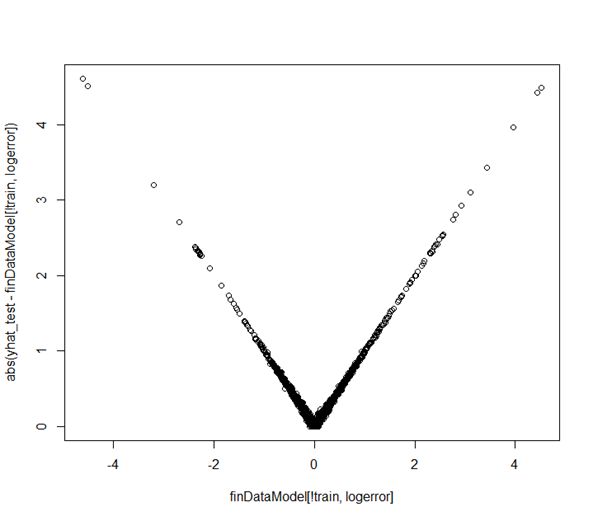
The predicted error versus the actual response is plotted in Figure 6. The graph is only provided for SVM
as this graph is similar for all the methods. The V-shape of the absolute error plot indicates that our prediction
only works well when the original estimation (Zestimate) is already accurate. When the original Zestimate is
Stat., Optim. Inf. Comput. Vol. 7, March 201972 PREDICTING HOME VALUE IN CALIFORNIA, UNITED STATES VIA MACHINE LEARNING MODELING
Figure 4. Summary of random forest with preprocess data set.
Figure 5. Visualized summary of MSE for each method.
Stat., Optim. Inf. Comput. Vol. 7, March 2019Y. HUANG 73
Table 2. Summary of MSE for each method.
linear regression tree boosting random forest SVM Baseline (sample variance)
0.026 0.06 0.21 0.08 0.024 0.025
problematic, our estimation will fail to predict. Moreover, the methods above tend to underestimate the Zestimate
prediction error. No method stands out. To some extent, it may conclude that Zestimate does provide a relative
accurate prediction.
Figure 6. Predicted error versus the actual response.
Through this experiment, it also concludes that feature selection is a very important process. Deleting features
with intuition can be very dangerous. To this end, tree-based methods are very useful when facing a model with
large number of features in home value prediction.
REFERENCES
1. J. McCarthy, M.L. Minsky, N. Rochester, C.E. Shannon, A Proposal for the Dartmouth Summer Research Project on Artificial
Intelligence, AI MAGAZINE, vol. 27, no. 4, pp. 12–14, 2006.
2. N. Cristianini, The road to artificial intelligence: A case of data over theory, New Scientist, 2016
3. A. Halevy, P. Norvig, F. Pereira, The Unreasonable Effectiveness of Data, IEEE Intelligent Systems, vol. 24, no. 2, pp. 8–12, 2009.
4. D. Goldberg, J. Holland,, Genetic Algorithms and Machine Learning, Machine learning, vol. 3, pp. 95–99, 1988.
5. W. Cai, J. Gong, N. Wu, 2.4GHZ Class F Power Amplifier for Wireless Medical Sensor Network, Proceedings of the 2nd World
Congress on New Technologies, 2016.
6. Z. Zhang, J. Ou, D. Li, S. Zhang, J. Fan, A thermography-based method for fatigue behavior evaluation of coupling beam damper,
Fracture and Structural Integrity, vol. 11, no. 40, 2017.
Stat., Optim. Inf. Comput. Vol. 7, March 201974 PREDICTING HOME VALUE IN CALIFORNIA, UNITED STATES VIA MACHINE LEARNING MODELING
7. E. Turban, J.E. Aronson, T.-P. Liang, Decision Support Systems and Intelligent Systems, Prentice-Hall, Inc., Upper Saddle River,
NJ, 2005.
8. W. Cai, L. Huang, W. Wen, 2.4GHZ Class AB Power Amplifier for Wireless Medical Sensor Network, International Journal of
Enhanced Research in Science, Technology & Engineering, vol. 5, no. 4, pp. 94–98, 2016.
9. Z. Zhang, J. Ou, D. Li, S. Zhang, Optimization Design of Coupling Beam Metal Damper in Shear Wall Structures, Applied Sciences,
vol. 7, no. 137, 2017.
10. D. Grant, E. Cherif, Analysis of e-business models in real estate, Electronic Commerce Research, 2013.
11. W. Cai, F. Shi, Design of low power medical device, International Journal of VLSI design & Communication Systems (VLSICS),
vol.8, no. 2, 2017.
12. D. Li, S. Zhang, W. Yang, W. Zhang, Corrosion Monitoring and Evaluation of Reinforced Concrete Structures Utilizing the
Ultrasonic Guided Wave Technique, International Journal of Distributed Sensor Networks, vol. 10, no. 9, 2014.
13. R.E. Lowrance, Predicting the Market Value of Single-Family Residential Real Estate, PhD Dissertation, 2015.
14. G. Hu, J. Wang, W. Feng, Multivariate Regression Modeling for Home Value Estimates with Evaluation Using Maximum Information
Coefficient, Software Engineering, Artificial Intelligence, Networking, SCI 443, pp. 69–81, 2013.
15. Vapnik, V, The Nature of Statistical Learning Theory, Springer-Verlag., 1995.
16. Shuichi Shinmura, The 95% confidence intervals of error rates and discriminant coefficients, Statistics, Optimization & Information
Computing, vol. 3, pp. 66–78, 2015.
17. J. Mu, F. Wu, A. Zhang, Housing Value Forecasting Based on Machine Learning Methods, Abstract and Applied Analysis, 2014.
Stat., Optim. Inf. Comput. Vol. 7, March 2019You can also read


