Property prices and bank lending in China
←
→
Page content transcription
If your browser does not render page correctly, please read the page content below
Journal of Asian Economics 18 (2007) 63–75

             Property prices and bank lending in China
                                       Qi Liang a,b,*, Hua Cao a
             a
                 Department of Finance, School of Economics, Nankai University, Tianjin 300071, China
                       b
                         Institute of Japanese Studies, Nankai University, Tianjin 300071, China
     Received 15 September 2006; received in revised form 20 November 2006; accepted 21 November 2006

Abstract
   This paper investigates the relationship between property prices and bank lending for the case of China
over the period 1999Q1–2006Q2. Under a high dimensional autoregressive distributed lag (ARDL)
framework with gross domestic product (GDP) and interest rate also being taken into account, we find
that there exists unidirectional causality running from bank lending to property prices, and that the causality
runs interactively through the error correction term from bank lending, GDP and interest rate to property
prices. Our findings have important policy implications.
# 2007 Elsevier Inc. All rights reserved.

JEL classification : E52; C32; G21

Keywords: Property prices; Bank lending; ARDL; China

1. Introduction

   The development of the property sector in China is significantly remarkable since China
adopted the economic reform policy in the late 1970s. The value added created by the property
sector has increased gradually, and property sector has made more and more contributions to the
economic growth. In the years 1953–1978, China’s gross domestic product (GDP) had increased
6.1% annually, in which property sector had increased 5% annually. Besides, the value added
created by property sector accounted about 2% in GDP and the property sector had contributed
1.83% to the economic growth. In the years 1978–2005, China’s GDP had increased 9.6%
annually, and the corresponding figures relating to the property sector had increased respectively

 * Corresponding author at: Department of Finance, School of Economics, Nankai University, Tianjin 300071, China.
Tel.: +86 22 2350 8544; fax: +86 22 2350 1816.
    E-mail addresses: liangqi@nankai.edu.cn (Q. Liang), caohua@nankai.edu.cn (H. Cao).

1049-0078/$ – see front matter # 2007 Elsevier Inc. All rights reserved.
doi:10.1016/j.asieco.2006.12.013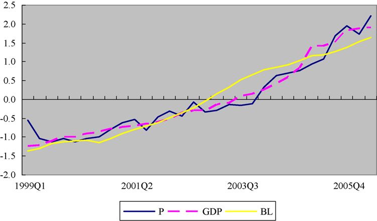
64                       Q. Liang, H. Cao / Journal of Asian Economics 18 (2007) 63–75

to 11.4%, 4.1% and 2.39%.1 Recently, the prominent position of property sector as a pillar
industry in the national economy has even been endorsed by the official documents of the State
Council. On the other hand, the property prices have been quite strong over the last decade.
Particularly, since 2004, the property prices have gone up extraordinarily. The annual growth
rates of property prices increased 15.1% and 19.5% in 2004 and 2005, comparing to respective
previous year. Some scholars pointed out that bank lending has played an important role in the
roaring property prices, e.g., the credit exposure of commercial banks to the property and
property-related sector had increased from only 3.6% in 1998 to 14.8% in 2004 and the mortgage
loan to total loan ratio had increased from only 0.59% in 1998 to 8.88% in 2005.2 These figures
have resulted growing interests among academics and policymakers to study the interactions
between property prices and bank lending, especially the possible responsiveness of property
prices to reserve rate and interest rate adjustments so that central bank may prevent the disruptive
effects of property prices shock on financial stability and the whole economy. Policymakers
appear to have taken the notice. On April 28, 2006, central bank raised the base lending rate from
5.58% to 5.85%. Moreover, central bank also raised the required reserve rate three times this year
on July 5, July 21 and August 15, up 0.5% each time. These measures appear to have certain
effects, as the growth rate of property-related investment started to head down in 2005.
Nevertheless, property prices, especially residential property prices, are rising as ever, although
at a relatively slower pace.
   From the viewpoint of policymakers, reliable and timely examination of the relationship
between property prices and bank lending could help them formulate effective policy decisions.
Moreover, market practitioners also need accurate estimations to make effective investment and
risk management decisions. Theoretically, there exists potentially bidirectional causality
between property prices and bank lending. On one hand, property prices may influence the
availability of bank lending via the wealth effect and the Tobin’s Q effect and the financial
accelerator effect (e.g., Bernanke & Gertler, 1999; Kiyotaki & Moore, 1997). Movements in
property prices may change the borrowing capacity and credit demand of corporations and
households. On the other hand, credit availability may also affect property prices, as increases in
credit availability may expand the demand for properties. So far, abundant international
evidences have documented the coincidence of property price cycles with bank lending cycles
(e.g., Zhu, 2003). Empirical studies of developed economies often find unidirectional causality
running from property prices to bank lending. Shimizu (2000) presents a theory of bank lending
and collateral to explain the banks’ lending behavior and the important role played by rising land
prices in Japan. Based on the estimated impulse-response functions, empirical analysis on the
relationships among land prices, bank loans and funds raised in the capital market indicates that
there exists causality between land prices and financial market activities, and loans to small and
medium-sized firms and funds raised in the capital markets are significantly affected by land
prices. In another study, using a number of indicators of land prices and bank lending, Shimizu
(2006) also finds unidirectional causality running from the former to the latter in the March 1956
to March 1999 periods in Japan. Gerlach and Peng (2005) investigate the long-run relationship
between bank lending and property prices in Hong Kong under a vector autoregressive
framework with multivariable such as property prices, bank lending, interest rate and gross

  1
    Data source: China’s property development condition and trend forecasting, China’s Property Development Fore-
casting Report 2006–2010, Macroeconomic Research Section, Development Research Center of State Council, China.
  2
    Data source: People’s Bank of China and Wind Database.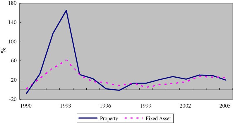
Q. Liang, H. Cao / Journal of Asian Economics 18 (2007) 63–75                                 65

domestic product (GDP),3 and find that the strong correlation between property prices and bank
lending appears to be due to bank lending adjusting to property prices, rather than the converse.
They suggest that excessive bank lending was not the root cause of the boom and bust cycles of
the property market in Hong Kong. In a similar study, Hofmann (2003) analyzes the direction of
causality between bank lending and property prices in 20 industrialized countries over the last
two decades. The long-run causality also appears to go from property prices to bank lending,
suggesting that property price cycles, reflecting changing beliefs about future economic
prospects, drive credit cycle. However, empirical studies on emerging market economies often
find that there exists an opposite unidirectional causality. Collyns and Senhadji (2001) find that
credit growth has a significant contemporaneous effect on residential property prices in a number
of Asian economies. Koha et al. (2005) investigate the Asian property price run-up and collapse
in the 1990s and identify financial intermediaries’ underpricing of the put option imbedded in
non-recourse mortgage loans as a potential cause for the observed price behavior.
   Unfortunately, most existing literature utilized cointegration approaches such as two-step
residual-based technique (Engle & Granger, 1987) or system-based reduced rank regression
method (Johansen, 1991), and might potentially suffer model specification problem due to the
fact that there is considerable doubt concerning the order of integration of variables such as
interest rate.4 In the presence of a mixture of stationary series and series containing a unit root,
standard statistical inference based on conventional likelihood ratio tests is no longer valid
(Harris, 1995). Recently, Pesaran, Shin, and Smith (2001) propose an autoregressive distributed
lag (ARDL) bounds test, which could be applied to cointegration identification irrespective of
whether the variables are integrated of order zero or integrated of order one. In addition, the main
body of the existing literature for the case of China focuses on subjective analysis, with a
conspicuous lack of studies being made to empirically determine this. Thus, within a high
dimensional ARDL framework, this paper attempts to fill the gap by examining the relationship
between property prices and bank lending in China, and the possible causality and causal
direction.
   The rest of the paper is organized as follows. Section 2 provides stylized facts about the
developments of property sector in China. Section 3 discusses the methodological issues. Section
4 presents the empirical results and policy implications. Section 5 concludes the whole paper.

2. Development in China’s property sector

   Before adopting the economic reform program in the late 1970s, China had implemented
welfarism housing system, characterized with low rent and allotment in kind. During the pre-
reform periods, property market was almost in non-existence. Therefore, we concentrate on the
development of China’s property sector in the post-reform period.5 In China, central government
plays a pivotal role in the residential property sector. According to the role played by the central
government in the residential property market, we classify the residential property sector

  3
    The real interest rate was not included since it did not enter significantly in the cointegrating vector (Gerlach & Peng,
2005, p. 469).
  4
    For example, Luintel and Khan (1999) find that half of the real interest rate series are stationary out of their sample
countries in a study focusing on the reassessment of the finance-growth nexus.
  5
    Since residential property sector has closely related to the households and its development has exerted a crucial
impact on households’ economic behavior, we focus on residential rather than commercial property sector. However, due
to the data availability, we have to use data from property sector instead of residential property sector in a few cases.
66 Q. Liang, H. Cao / Journal of Asian Economics 18 (2007) 63–75
development into three stages in the post-reform period.6 The first stage started in June 1980,
symbolized by the publicized National Construction Meeting Report, which raised the curtain on
housing reform by allowing households themselves to build house, buy house and own house.
Moreover, government budget began to afford only part of the construction and maintenance
costs, with the rest shared between households and their affiliations. Funds from financial
institutions were also allowed to enter the residential property sector, e.g., China Construction
Bank (named China People’s Construction Bank at that time) started to issue property-related
credit and a few residential saving banks have been set up in coastal areas. The residential
property sector underwent its preliminary development. In May 1990, Regulations on Sell and
Transfer the Right of Use of State-owned Land in City and Town Areas was publicized, which put
forward that it is allowable to sell and transfer the right of use of state-owned land in city and
town areas. Therefore, a tradable property market began to form. The Regulations stipulates that
local government authority could retain part of the revenue from the state-owned land transfer
and sales, thus, foreshadowing the property boom in the coming years. At this stage, government
attempted to withdraw the residential property sector through housing reform. The second stage
started in 1992 when Deng Xiaopeng called for speeding up the rate of economic reform, which
led to a major ideological breakthrough that for the first time China’s socialist market economy
was endorsed by the central government. Soon after, the residential property prices were opened
to the market and a number of examinations and approval rights were being gradually
deregulated. These measures suddenly drove the residential property sector into quick
development lane, manifested by high growth rate of residential property-related investments,
significant space increases in land development, establishment of numerous new property-related
firms, active property market with huge trading volumes and rising prices. The investments in
property-related development increased 117.5% in 1992 and 165% in 1993. The proportion of
property-related development investments in total fixed asset investments also increased
suddenly from 9.0% in 1992 to 14.8% in 1993. There were only 1991 property-related
development companies in 1986, while the new establishments in only one year in 1992 reached
8438. Unfortunately, this property boom soon brought about a lot of problems, such as runaway
land supply and inequitable return distribution. Accordingly, central government set about in July
1993 to formulate macro regulations towards property sector, which came into effect
immediately, as the annual growth rate of property-related development investments dropped
133.2% in 1994 comparing to that of the previous year. In 1996, the annual growth rate further
dropped to only 2.1% and in 1997 it even turned out to be negative (1.2%). At this stage,
although central government tried to withdraw the residential property market as a key financing
supplier, its policy caused to a certain degree the property boom-burst cycle. The latest stage
started in July 1998 when central government publicized the Notice on the Deepening of Housing
Reform and Fasten Housing Construction, which stipulated (i) stopping house allot in kind and
implementing progressively house allot by money; (ii) establishing a multi-layer house supplying
system in city and town with the economically suitable house to be the mainstay; (iii) developing
the house financing system and raising the residential property trading market. The government
role in the residential property market transformed to provide favorable policy and fund subsidy
only to economically suitable house. This symbolized that market began to function as an
6
So far, there is no generally accepted standard among economists on the classification of residential property sector. A
few scholars used to classify the residential property market development in the post-reform periods into three or four
stages according to the level or growth rate of property-related investments.Q. Liang, H. Cao / Journal of Asian Economics 18 (2007) 63–75 67
Fig. 1. Growth rates of investments in property-related development and total fixed assets.
invisible hand in the residential property financing system. At the same year, the annual growth
rate of property-related development investment began to rise and the rate has kept about 20%
since then.
Fig. 1 plots the annual growth rate of investment in property-related development and in total
fixed assets during the 1990–2005 periods. It is clear that the turning points in the two series are
generally in accordance with the classified development stages of the residential property sector.
Besides, it shows that at the second stage, the growth rates of property-related development
investments were lower than those of investments in total assets in most of the years, while the
situation reversed at the third stage. However, it is worthwhile to note that recently in 2005 the
growth rate of property-related development investments was lower than that of the investments
in total assets for the first time in six consecutive years. This might ascribe to the tight regulations
implemented since 2003 with an objective to contain the heated investments and roaring
residential property price.
Similar to the stages of residential property sector development, the movements in residential
property prices can also be classified into three stages (see Fig. 2). Interestingly, the price
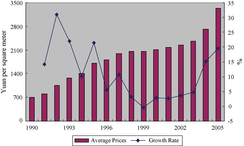
Fig. 2. Average residential property prices and its annual growth rate.68 Q. Liang, H. Cao / Journal of Asian Economics 18 (2007) 63–75
Table 1
Descriptive data on outstanding of household mortgage loan and total loan
Year Household mortgage Growth Total loan Growth Mortgage-total
loan outstanding rate outstanding rate (%) loan ratio (%)
(billion Yuan) (%) (billion Yuan)
1998 51.40 170.5 8652.41 15.5 0.59
1999 135.77 164.2 9373.43 8.3 1.45
2000 337.69 148.7 9937.11 6.0 3.39
2001 559.79 65.8 11231.47 13.0 4.98
2002 826.87 47.7 13980.30 24.5 5.89
2003 1177.97 42.5 16977.10 21.4 6.94
2004 1592.23 35.2 18856.60 11.1 8.44
2005 1836.60 15.3 20683.80 9.7 8.88
movements generally lag behind the corresponding property sector development by one or two
years.
At the first stage in the 1990–1992 periods, residential property prices rose steadily due to the
factors that in response to the macroeconomic conditions, commercial banks developed new
financial products providing firms with both short-term working capital and long-term fixed asset
investment fund, and also providing households with consuming-related loan. Beside, each
special bank set up its owned property credit section. In 1992, the growth rate of the residential
property prices reached 30.9%, the highest level ever have since the housing reform started. At
the second stage in the 1993–1999 periods, central government began in 1993 to readjust and
rectify the property sector through implementation of restrictive monetary policies. Central bank
required each special bank to draw up credit plan and fixed asset investment plan for every new
property-related loan. The tight regulation led the growth rate of the residential property prices
touching bottom in 1996, and even turning out to be negative (0.5%) in 1999. Since 1996, the
central bank has embarked to apply expansive monetary policy by lifting the tight regulation and
lowering interest rates progressively. Particularly, the Regulations on Mortgage Loan to
Households publicized in 1998 stipulated that all commercial banks could grant mortgage loans
to the households, thus, bring in competitive mechanism into the house financing market used to
be monopolized by China’s Construction Bank. Hence, the amount of mortgage loan increased
immediately and explosively. Table 1 presents the outstanding of household mortgage loan and
total loan of the financial institutions in the 1998–2005 periods. Data indicate that the average
annual growth rate of the household mortgage loan outstanding reached 161.13% in the first 3
years. Although stepping down gradually in recent years, the growth rates of the household
mortgage loan outstanding are still significantly higher than those of the total loan outstanding.
Moreover, the mortgage loan to total loan ratio has also risen up steadily since 1998.
On the other hand, commercial banks have involved more and more deeply in the residential
property financing market, encouraged mainly by the lower interest rate. Table 2 presents the
sources of funds of enterprises for property development in the 1997–2004 periods. Data show
that funds from the state budgetary appropriation, bonds and foreign investment have decreased
gradually in these years, while funds from domestic loan, self-raising fund and others have
increased constantly, with the latter there items accounting averagely 22.62%, 27.78% and
45.05%, respectively.
Although data show that domestic bank credit only accounts for about one fifth in the sources
of funds of enterprises for property development, it covers important fact because of the advanceQ. Liang, H. Cao / Journal of Asian Economics 18 (2007) 63–75 69
Table 2
Source of funds of enterprises for property development (one hundred million Yuan)
Year Total funds State budgetary Domestic Bonds Foreign Self-raising Others
appropriation loans investment fund
1997 3817.07 12.48 911.19 4.87 460.86 972.88 1454.79
1998 4414.94 14.95 1053.17 6.23 361.76 1166.98 1811.85
1999 4795.90 10.05 1111.57 9.87 256.60 1344.62 2063.20
2000 5997.63 6.87 1385.08 3.48 168.70 1614.21 2819.29
2001 7696.39 13.63 1692.20 0.34 135.70 2183.96 3670.56
2002 9749.95 11.80 2220.34 2.24 157.23 2738.45 4619.90
2003 13196.92 11.36 3138.27 0.55 170.00 3770.69 6106.05
2004 17168.77 11.81 3158.41 0.19 228.20 5207.56 8562.59
Fig. 3. Property prices, bank lending and GDP (1999Q1–2006Q2).
house booking system implemented nowadays in the residential property market, i.e., self-raising
funds are mainly transformed from house sales revenues in which most origin from the bank
mortgage loan. Together, bank lending may account for as many as 55% in the property
development (Yi & Huang, 2006). Due to the lagged effects of the expansive policy, together with
the low interest rate and increased bank lending, the residential property prices moved upward
once again in 2000 and in the third stage starting from 2000, the average annual growth rate
reaches 8.1%, especially in the last two years the prices rose rapidly with annual growth rate of
15.1% and 19.5%, respectively in 2004 and 2005. Fig. 3 plots the quarter property prices, bank
lending and GDP in real terms in the 1999Q1–2006Q2 periods.7 Bank lending and output appear
more stable than property prices and this finding is compatible with the existing literature
(Gerlach & Peng, 2005). However, since 2004, it seems that both property prices and GDP have
increased more rapidly than bank lending.
7
We normalized the real variables by demeaning them and dividing through with their standard deviations in order to
facilitate comparison.70 Q. Liang, H. Cao / Journal of Asian Economics 18 (2007) 63–75
3. Econometric methodology
We employ the autoregressive distributed lag bounds testing approach suggested by Pesaran
et al. (2001) as the most appropriate model specification to carry out cointegration analysis among
property prices, bank lending, GDP and interest rate. The bounds testing approach has numerous
advantages. Besides that it can be applied irrespective of whether the variables are stationary or
nonstationary, bounds testing approach has better small sample properties (Narayan & Smyth,
2005). Moreover, a dynamic error correction model (ECM) can be derived from ARDL through a
simple linear transformation (Banerjee, Dolado, Galbraith, & Hendry, 1993). The ECM integrates
the short-run dynamics with the long-run equilibrium without losing long-run information.
The ARDL approach to cointegration involves estimating the conditional error correction
version of the ARDL model as follows:
X
p X
p
Dyt ¼ p10 þ p11 yt1 þ p12 xt1 þ g i1 Dyt1i þ a j1 Dxt j1 þ e1t (1A)
i1¼1 j1¼0
X
p X
p
Dxt ¼ p20 þ p21 xt1 þ p22 yt1 þ g i2 Dxti2 þ a j2 Dyt j2 þ e2t (1B)
i2¼1 j2¼0
where y and x are model variables, and et is assumed to be white noise error processes. The ARDL
approach estimates ( p + 1)k number of regressions for each equation in order to obtain optimal
lag length for each variable, where p is the maximum number of lag to be used and k is the
number of variables in the equation. The optimal lag structure of the first difference regressors is
selected by the Schwarz–Bayesian criteria (SBC) to ensure an absence of serial correlation in the
estimated residuals.8 Following Pesaran et al. (2001), two separate statistics are employed to
‘bounds test’ for the existence of a long-run relationship, e.g., for Eq. (1A): an F-test for the joint
significance of the coefficients of the lagged levels in Eq. (1) (so that H0:p11 = p12 = 0), and a t-
test for the significance of the coefficient of the lagged level of dependent variable in Eq. (1) (so
that H0:p11= 0). Two asymptotic critical value bounds provide a test for cointegration when the
independent variables are I(d) (where 0 d 1): a lower value assuming the regressors are I(0),
and an upper value assuming purely I(1) regressors. If the test statistic exceeds the upper critical
value, we can conclude that a long-run relationship exists regardless of whether the underlying
orders of integration of the variables are zero or one. If the test statistics fall below the lower
critical values we cannot reject the null hypothesis of no cointegration. However, if the statistics
fall between these two bounds, inference would be inconclusive.
Then, the long-run relationship is estimated using the selected ARDL model. If variables are
cointegrated in case y is used as dependent variable, then the conditional long-run model can then
be produced from the reduced form solution of Eq. (1A), when the first-differenced variables
jointly equal zero, i.e., Dy = Dx = 0. Thus,
yt ¼ Q0 þ Q1 xt þ mt (2)
where Q0 = p10/p11;Q1 = p12/p11, and mt is random error. The long-run coefficients are
estimated by the ARDL model in Eq. (1) by OLS. When there is a long-run relationship
8
SBC is known as selecting the smallest possible lag length to specify a parsimonious model.Q. Liang, H. Cao / Journal of Asian Economics 18 (2007) 63–75 71
between variables, there exists an error correction representation. Therefore, the error
correction model is estimated, and can be used to conduct the conventional Granger non-
causality tests.
Xh
yt g g 12i yti c v
ð1 LÞ ¼ ð1 LÞ 11i þ ECTt1 þ 1t (3)
xt i¼1
g 21i g 22i xti u v2t
where (1 L) is the difference operator, ECTt1 is the lagged error-correction term derived from
Eq. (2) and this term is included only if the variables are cointegrated. The lag lengths are selected
by the general-to-specific approach. The t-statistics on the coefficients of the lagged error-
correction term indicates the significance of the long-run causal effect while the F-statistics or t-
statistics on the lagged explanatory variables indicates the significance of the short-run causal
effect.
4. Estimation results
The study employs quarter time series data from 1999Q1–2006Q2 and all data are extracted
from Wind Database and Information Center of Development Research Center of State Council.
The period for the empirical analysis was dictated by data availability of the quarter property
prices. The real property prices (P), real GDP (Y), real total bank lending (BC) and the real
interest rate (R) are derived by dividing nominal values with consumer price index (CPI) with
1999Q1 as the base.9 In addition, all variables except interest rate were seasonally adjusted and
were then transformed into natural logs. The reason to choose total bank lending instead of
property-related lending is that in addition to provide residential mortgage loans, banks also lend
extensively to the corporate sector for construction and property development. Moreover, there is
anecdotal evidence that part of the other loans to the corporate and household sectors were
effectively for property-related investment.
A four-stage procedure is followed to analyze the long-run relationship between property
prices, bank lending, GDP and interest rate.10 First, we test the order of integration using PP unit-
root test. Second, we conduct the bounds test for the null hypothesis of no cointegration. Third,
we model the long-run relationship among variables using the estimated coefficients from the
selected ARDL specification. Forth, we carry out dynamic analysis using the error correction
model.
Unit-root test statistics indicate that P, BC and Y are trend non-stationary, significant at 5%
level or better, while R is level stationary.11 The first differences of P, Y and BC are tested to be
stationary. Hence, series P, Y and BC are integrated of order one and series R are integrated of
order zero. A mixture of I(1) and I(0) variables show that the ARDL framework is a particularly
relevant application given the time series properties of our data.
9
The interest rate denotes lending rate in one year.
10
The correlation coefficient between bank lending and lending rate is 0.0165 during the sample periods, thus, we
conclude that including both of them in the model might not give rise to multicolinearity problem. In addition, as
indicated by the referee, it is better to take into account the impact of administrative measures such as window guidance
on lending to the property sector, however, these factors are difficult, if not impossible, to be quantified.
11
Following standard practice in unit-root test literature and judging from the visual inspection of the series, we include
a linear deterministic trend in the unit-root test for series P, BC and Y.72 Q. Liang, H. Cao / Journal of Asian Economics 18 (2007) 63–75
In order to test the existence of long-run equilibrium relationships among variables, the
following unrestricted error correction models (UECM) are investigated:
Xp X
p
DPt ¼ p10 þ p11 Pt1 þ p12 Y t1 þ p13 BCt1 þ p14 Rt1 þ g i1 DPt1i þ a j1 DY t j1
i1¼1 j1¼0
X
p X
p
þ $s1 DBCts1 þ fl1 Rtl1 þ e1t (4A)
s1¼0 l1¼0
X
p X
p
DY t ¼ p20 þ p21 Y t1 þ p22 Pt1 þ p23 BCt1 þ p24 Rt1 þ g i2 DY ti2 þ a j2 DPt j2
i2¼1 j2¼0
X
p X
p
þ $s2 DBCts2 þ fl2 Rtl2 þ e2t (4B)
s2¼0 l2¼0
X
p
DBC t ¼ p30 þ p31 BCt1 þ p32 Pt1 þ p33 Y t1 þ p34 Rt1 þ g i3 DBCti3
i3¼1
X
p X
p X
p
þ a j3 DY t j3 þ $s3 DPts3 þ fl3 Rtl3 þ e3t (4C)
j3¼0 s3¼0 l3¼0
X
p X
p
DRt ¼ p40 þ p41 Rt1 þ p42 Pt1 þ p43 Y t1 þ p44 BCt1 þ g i4 DRti4 þ a j4 DPt j4
i4¼1 j4¼0
X
p X
p
þ $s4 DY ts4 þ fl4 BCtl4 þ e4t (4D)
s4¼0 l4¼0
where the lagged level terms represent the long-run relationship while the terms with the
summation signs correspond to the error correction dynamics. We include a minimum of one lag
and a maximum of four to ensure lagged explanatory variables are present in the ECM in the
bounds test since the costs of over-parameterization in terms of efficiency loss is marginal
(Gonzalo, 1994). The results of the bounds test for cointegration are presented in Table 3. The
bounds test statistics indicate cointegration are present when property prices or output is
the dependent variable due to the fact that both tp(PjY, BC, R) and ty(YjP, BC, R) are higher
than the upper bound critical value at the 5% level, and meanwhile both F p(PjY, BC, R) and
F Y(YjP, BC, R) are higher than the upper bound critical value at the 1% level.
Since we are mainly interested in the correlation relationship and causality between property
prices and bank lending, we focus on the cointegration relationship when property price is
Table 3
Bounds test statistics for cointegration
t-statistics F-statistics
**
tp(PjY, BC, R)= 4.2124 Fp(PjY, BC, R)= 6.7371***
ty(YjP, BC, R)= 4.1231** Fy(YjP, BC, R)= 9.2045***
tBC(BCjP, Y, R)= 1.3638 FBC(BCjP, Y, R)= 1.5961
tR(RjP, Y, BC)= 3.4481 FR(RjP, Y, BC)= 5.0473
Note: Bounds test statistics are compared with critical values tabulated in Pesaran et al. (2001, p. 300, p. 303). The
symbols (***) and (**) indicate rejection of the null hypothesis at 1% and 5%, respectively.Q. Liang, H. Cao / Journal of Asian Economics 18 (2007) 63–75 73
dependent variable. Hence, the conditional long-run relationship could be produced from the
reduced form solution of Eq. (4A) as follows:
P ¼ 1:2926 þ0:5615Y þ 0:0630BC þ 0:0056R (5)
where the symbols (***) and (**) indicate the significance at 1% and 5% level. Generally speaking,
since increasing bank lending and income, and decreasing interest rate will drive up the property
prices, we expect the coefficients of BC and Y to be positive while the coefficient of R negative. The
long-run test results reveal that the GDP (income) is the major factor that affects the property prices
while bank lending is another less important factor. These findings are as expected and in
accordance with a few literatures. However, surprisingly and interestingly, the coefficient of
interest rate turns out just opposite to our expectations. This paradox is pretty obscure. It shows that
at least in the examined sample periods, the property price movements in China has no sensitivity to
the changes of the real interest rate. Perhaps this might be ascribed to (i) property sector earns
exorbitant profits so that although a restrictive monetary policy is in place, private capital and
financial capital still pour into the property industry, driving up the property prices; (ii) real interest
rate does not reflect the short-run opportunity cost due to the somewhat financial depression
implemented in China and the rate is further distorted by the lower inflation. Undoubtedly, this
result needs further examination. Li and Yang (2005) find a negative relationship between property-
related investment and real interest rate. We agree with them to the part that interest rate, in
particular the short-term interest rate, is not an effective way to control property prices.
At last, we carry out the Granger non-causality tests. Although GDP and bank lending appear
to be the long-run forcing variables based on the ARDL model, this is only a necessary but not
sufficient condition for rejecting Granger non-causality. The ARDL–ECM are constructed as
follows:
2 3 2 32 3 2 3
Pt g 11i g 12i g 13i g 14i Pti c
6 Yt 7 X h 6 g 21i g 22i g 23i g 24i 76 Y ti 7 6 u 7
ð1 LÞ6 7
4 BCt 5 ¼ ð1 LÞ6
4 g 31i
76 7 þ 6 7ECTt1
i¼1
g 32i l33i g 34i 54 BCti 5 4 h 5
Rt l41i g 42i l43i g 44i Rti ’
2 3
v1t
6 v2t 7
þ6 7
4 v3t 5 (6)
v4t
In order to obtain the parsimonious model, the lag lengths are selected by the general-to-
specific methods by removing insignificant variables step by step, starting with the most
insignificant one as indicated by the t-ratios. Then, we test the significance of the coefficient of
the lagged error correction term and joint significance of the lagged differences of the
explanatory variables. Table 4 presents the short-run and long-run Granger causality within the
error correction mechanism.
Test statistics show the coefficients on the error correction terms are highly significant, thus,
confirming the long-run relationship among variables, as Granger, Huang, and Yang (2000)
suggests, a significant error correction term is indicative of long-run causality. Furthermore, F-
statistics or t-statistics on the lagged explanatory variables indicates in the short-run GDP
(income) also causes property prices while there were no causal relationships running from bank
lending and interest rate to property prices, together implying that changes in property prices are74 Q. Liang, H. Cao / Journal of Asian Economics 18 (2007) 63–75
Table 4
Results of Granger causality tests
Dependent variable DP DY DBC DR ECT
**
DP – 2.5347 0.6288 0.1327 5.7236***
DY 2.5931 – 2.9485* 2.7824* –
DBC 0.9482 1.6159 – 2.5924** –
DR 6.4363*** 1.8648 0.7177 – –
Note: The symbols (***); (**) and (*) indicate rejection of the null hypothesis at 1%, 5% and 10%, respectively.
a function of disequilibrium in the cointegrating relationship. In other words, the causality runs
interactively through the error correction term from bank lending, GDP (income) and interest rate
to property prices.
Central government in China now is aiming to control property prices. Therefore, our findings
have important policy implications. On the one hand, empirical results appear to offer little
support to the view that interest rate might be an effective way to exert impacts on the property
price movements. On the other hand, the weak impacts of bank lending on property prices
suggest that central government might prevent property prices from further rising to a certain
degree through formulating tight credit policies. In addition, we warn that, as property
development funds depend more and more on bank lending, and bank profits rely more and more
on property or property-related sectors, bank itself may face increasing financial risk.12
Particularly, the sharp falling property prices may have devastating impacts on local financial
institutions since many of them have high concentration in the local property sector. The collapse
of property prices could easily drag down these local banking institutions and generate systemic
risk for the whole financial system. As a result, it is crucial for managers and financial regulators
to measure accurately the risk exposure of banks and to make sure that such risk does not
jeopardize the stability of the financial system.13
5. Conclusion
By implementing a high dimensional ARDL framework to the quarter data of China in her
1999Q1–2006Q2 periods, we have empirically examined the long-run relationships and
evaluated the causality between property prices and bank lending while also taken GDP and
interest rate into account. We find that unidirectional causality exists running from bank lending
to property prices, conclusions departing distinctively from previous empirical studies on
developed economies. Moreover, in the long run, bank lending, GDP (income) and interest rate
Granger cause property prices, meaning that causality run interactively through the error
correction term from income, bank lending and interest rate to property prices. Our findings have
important policy implications. Interest rate might not be a valid and sufficient tool to control the
property prices. However, government may partly accomplish its objective of controlling
property prices through tight credit policy.
12
Shimizu (1997) points out that the dominant position of banks in Japan’s financial market and the lack of an effective
system of credit risk sharing through the capital market were the fundamental structures that brought about the ensuing
financial crisis.
13
Gerlach and Peng (2005) suggest that prudential regulation and risk controls by banks could limit the exposure and
vulnerability of the banking sector to swings in property prices.Q. Liang, H. Cao / Journal of Asian Economics 18 (2007) 63–75 75
Acknowledgements
We are grateful to the constructive comments and detailed suggestions of Chi Hung Kwan,
Yoshinori Shimizu, Eiji Ogawa, Dar-Yeh Hwang, Naoyuki Yoshino and the insights of
participants at International Conference on Financial System Reform and Monetary Policies in
Asia held on September 15–16, 2006 at Hitotsubashi University in Tokyo, Japan. We would also
like to thank Yu-Cao Liu, Dong-Liang Yang, Jun-Shou Wang, Ya-Hui Yang and Jian-Zhou Teng
for helpful comments and seminar participants at Nankai University. This work was funded by a
research grant (06JA790057) from the Ministry of Education. Any errors or omission are solely
our own. An earlier draft of this paper was circulated with the title ‘‘The Impact of Monetary
Policy on Property Prices: Evidence from China’’.
References
Banerjee, A. J., Dolado, J., Galbraith, J. W., & Hendry, D. (1993). Co-integration, error correction, and the econometric
analysis of non-stationary data. Oxford: Oxford University Press.
Bernanke, B., & Gertler, M. (1999). Monetary policy and asset price volatility. Federal Reserve Bank of Kansas City
Economic Review, 84, 17–52.
Collyns, C., & Senhadji, A., 2001. Lending booms, real estate bubbles and the Asian crisis. IMF Working Paper No. 02/20.
Engle, R. F., & Granger, C. W. (1987). Cointegration and error-correction representation, estimation, and testing.
Econometrica, 55, 251–276.
Gerlach, S., & Peng, W. S. (2005). Bank lending and property prices in Hong Kong. Journal of Banking and Finance, 29,
461–481.
Gonzalo, J. (1994). Five alternative methods of estimating long-run equilibrium relationships. Journal of Econometrics,
60, 203–233.
Granger, C., Huang, B., & Yang, C. (2000). A bivariate causality between stock prices and exchange rates: evidence from
recent Asian flu. The Quarterly Review of Economics and Finance, 40, 337–354.
Harris, R. (1995). Using cointegration analysis in econometric modeling. London: Prentice Hall.
Hofmann, B., 2003. Bank lending and property prices: Some international evidence. The Hong Kong Institute for
Monetary Research Working Paper No. 22.
Johansen, S. (1991). Estimation and hypothesis testing of cointegration vectors in Gausian vector autoregression models.
Econometrica, 59, 551–580.
Kiyotaki, N., & Moore, J. (1997). Credit cycles. Journal of Political Economy, 105, 211–248.
Koha, W. T. H., Marianoa, R. S., Pavlovb, A., Phanga, S. Y., Tana, A. H. H., & Wachterc, S. M. (2005). Bank lending and
real estate in Asia: market optimism and asset bubbles. Journal of Asian Economics, 15, 1103–1118.
Li, Y. J., & Yang, Y. (2005). The effect of interest rate and money supply impose on real estate investment in China: an
empirical analysis. Journal of Xi’an Institute of Finance and Economics, 18, 47–51.
Luintel, K. B., & Khan, M. (1999). A quantitative reassessment of the finance–growth nexus: evidence from a multivariate
VAR. Journal of Development Economics, 60, 381–405.
Narayan, P. K., & Smyth, R. (2005). Electricity consumption, employment and real income in Australia evidence from
multivariate Granger causality test. Energy Policy, 33, 1109–1116.
Pesaran, M. H., Shin, Y., & Smith, R. J. (2001). Bounds testing approaches to the analysis of level relationships. Journal of
Applied Econometrics, 16, 289–326.
Shimizu, Y. (1997). Nippon no Kinyu to Shiji Mechanism [The Japanese Financial Market and the Market Mechanism].
Tokyo: Toyo Economic Publishing House.
Shimizu, Y., 2000. Convoy Regulation, Bank Management, and the Financial Crisis in Japan. In Mikitani, R., and Posen,
A.S., Eds. Japan’s Financial Crisis and Its Parallels to U.S. Experience, Special report 13, Institute for International
Economics, 57–99.
Shimizu, Y., 2006. Fudousan kagaku to kinyuushijyou [Property Prices and Financial Market], Kinyuu Keizai Kenkyu
[Financial Economics Research] 23, 1–14.
Yi, X.R., & Huang, Y., 2006. Current house payment in advance system leads to high residential property prices. Shanghai
Securities News, July 14.
Zhu, H.B., 2003. The importance of property markets for monetary policy and financial stability. BIS paper No. 21.You can also read