Public Debt Dynamics in New Zealand - Melissa Piscetek New Zealand Treasury Working Paper 19/01 - Treasury NZ

Public Debt Dynamics in New Zealand

Melissa Piscetek

New Zealand Treasury Working Paper 19/01

July 2019

 DISCLAIMER
 The views, opinions, findings, and conclusions or recommendations expressed in this
 Working Paper are strictly those of the author(s). They do not necessarily reflect the views
 of the New Zealand Treasury or the New Zealand Government. The New Zealand Treasury
 and the New Zealand Government take no responsibility for any errors or omissions in, or
 for the correctness of, the information contained in these working papers. The paper is
 presented not as policy, but with a view to inform and stimulate wider debate.

 i

NZ TREASURY Public Debt Dynamics in New Zealand
WORKING PAPER 19/01

MONTH/YEAR July 2019

AUTHOR Melissa Piscetek
 1 The Terrace
 Wellington
 New Zealand
 Email melissa.piscetek@treasury.govt.nz

ISBN (ONLINE) 978-1-98-858056-2

URL Treasury website at July 2019:
 https://treasury.govt.nz/publications/wp/wp-19-01

ACKNOWLEDGEMENTS The author would like to thank Matthew Bell, Andrew Binning,
 Anna Hamer-Adams, Angus Hawkins, Thomas Helbling,
 Robert Kirkby, Oscar Parkyn and Eric Tong for their comments
 and feedback on earlier drafts of the paper.

NZ TREASURY New Zealand Treasury
 PO Box 3724
 Wellington 6008
 NEW ZEALAND
 Email information@treasury.govt.nz
 Telephone 64-4-472 2733
 Website www.treasury.govt.nz

Abstract
This paper develops a framework to decompose the change in New Zealand’s public
debt ratio into four component effects: the primary balance, real GDP growth, real
interest rates, and exchange rates. We study New Zealand's debt dynamics over three
periods: the decade after the Global Financial Crisis (2008 – 2018), the five-year
forecasts (2019 – 2023), and the medium-term projections (2024 – 2033). We find
asymmetry between the component effects of the debt dynamics on New Zealand's
public debt ratio. The primary balance is the larger contributor to the public debt ratio
(either positive or negative), while the automatic debt dynamics (the interest-growth
differential and exchange rates) are relatively benign.

KEYWORDS Public debt; debt dynamics; fiscal policy, debt sustainability, fiscal
 sustainability.

 W P 19/01 | Public D ebt D ynamics i n N ew Zeal and i

Executive Summary
We establish a framework to analyse New Zealand’s public debt dynamics, by
augmenting the Fiscal Strategy Model (FSM) with a debt dynamics model. We apply the
framework to study New Zealand’s public debt ratio in recent history, and to project the
dynamics into the future. This contributes to the literature on debt dynamics by
formalising an accounting framework to study New Zealand's debt dynamics.

We find asymmetry between the component effects of the debt dynamics on New
Zealand's public debt ratio. The primary balance is the larger contributor to the public
debt ratio (either positive or negative), while the automatic debt dynamics (the interest-
growth differential and the exchange rate effect) are relatively benign. This pattern may
continue. Declining global real interest rates have affected public debt dynamics, and the
Treasury forecasts that low interest rates will persist over the next five years.

Since 2008, the primary balance had the largest effect on gross public debt levels in New
Zealand. In the years following the Global Financial Crisis (GFC) and Canterbury
earthquakes, public debt rose sharply. The Government's fiscal response reduced gross
debt from 2013. Across the forecast years (2019 to 2023), the gross debt ratio is
expected to decline due to forecast primary surpluses. The medium-term projections
(2024 to 2033) show a slightly different trend. Although the gross debt ratio is expected
to be lower by 2033, we project a deteriorating primary surplus and increasingly
unfavourable automatic debt dynamics. These dynamics are partly driven by the
assumption that government bond rates will return to their historical average. Although
outside the scope of this paper, there is some evidence that bond yields will remain low.
If this is the case, it may alleviate concerns about the automatic debt dynamics in the
projection period.

 W P 19/01 | Public D ebt D ynamics i n N ew Zeal and ii

Contents
Abstract ............................................................................................................... i
Executive Summary ........................................................................................... ii
1 Introduction............................................................................................... 1
2 Sustainability and debt dynamics ........................................................... 3
 2.1 Measures of sustainability .............................................................................. 3
3 Analytical framework ................................................................................ 8
 3.1 Methodology ................................................................................................... 8
 3.2 Data ....................................................................................................... 11
4 Results .................................................................................................... 12
 4.1 History: 2008 to 2018 .................................................................................... 12
 4.2 The forecasts: 2019 to 2023 ......................................................................... 16
 4.3 The projections: 2024 to 2033 ...................................................................... 20
 4.4 Scenario analysis .......................................................................................... 23
5 Conclusion .............................................................................................. 26
Appendix 1: The solvency condition .............................................................. 30
Appendix 2: The debt dynamics ..................................................................... 32
 With no foreign currency denominated debt ........................................................... 32
 With foreign currency denominated debt ................................................................ 34
Appendix 3: Assumptions & variables ........................................................... 37
 History: 2008 to 2018 .............................................................................................. 37
 The forecasts: 2019 to 2023 ................................................................................... 37
 The projections: 2024 to 2033 ................................................................................ 38
 Downside scenario .................................................................................................. 38
Appendix 4: Results ........................................................................................ 39
 History: 2008 to 2018 .............................................................................................. 39
 The forecasts: 2019 to 2023 ................................................................................... 39
 The projections: 2024 to 2033 ................................................................................ 40
 Downside scenario .................................................................................................. 40

 W P 19/01 | Public D ebt D ynamics i n N ew Zeal and iii

List of Tables
Table 1: Key economic projection assumptions .................................................................. 9
Table 2: Data sources ....................................................................................................... 11
Table 3: Debt decomposition............................................................................................. 13
Table 4: Debt decomposition............................................................................................. 17
Table 5: Debt decomposition............................................................................................. 20
Table 6: Debt decomposition............................................................................................. 24

List of Figures
Figure 1: Gross debt-to-GDP .............................................................................................. 1
Figure 2: Core Crown debt-to-GDP ................................................................................... 12
Figure 3: The debt dynamics ............................................................................................. 14
Figure 4: Automatic debt dynamics (ø) Real interest and growth (r and g) ................... 14
Figure 5: US Government and New Zealand Government nominal ten-year bond rates . 15
Figure 6: Primary balance & debt stabilising primary balance .......................................... 16
Figure 7: Core Crown debt-to-GDP ................................................................................... 17
Figure 8: The debt dynamics ............................................................................................. 18
Figure 9: Automatic debt dynamics (ø) Real interest and growth (r and g) ................... 19
Figure 10: Primary balance & debt stabilising primary balance ........................................ 19
Figure 11: Core Crown debt-to-GDP ................................................................................. 20
Figure 12: The debt dynamics ........................................................................................... 21
Figure 13: Automatic debt dynamics (ø) Real interest and growth (r and g) ................. 21
Figure 14: Primary balance & debt stabilising primary balance ........................................ 22
Figure 15: Core Crown debt to GDP ................................................................................. 23
Figure 16: The debt dynamics ........................................................................................... 24
Figure 17: Automatic debt dynamics (ø) Real interest and growth (r and g) ................. 25
Figure 18: Primary balance & debt stabilising primary balance ........................................ 25

 W P 19/01 | Public D ebt D ynamics i n N ew Zeal and iv

Public Debt Dynamics in New Zealand

1 Introduction
New Zealand experienced a cycle of public debt accumulation over the past decade. In
the wake of the Global Financial Crisis (GFC), and compounded by the Canterbury
earthquakes of 2010 and 2011, core Crown debt-to-GDP (a gross debt measure)
increased by about 20 percentage points, reaching a peak of 40 percent of GDP in 2013.
In 2011, the Government targeted a return to Budget surplus by fiscal year 2015. This
target was achieved mainly through slowing the growth of nominal spending so that
expenditure-to-GDP declined (Philip, Bose & Sullivan 2017). Since then, debt levels have
reduced and, at the time of writing, core Crown debt is at 34 percent of GDP. The
New Zealand Treasury (the Treasury) forecasts that core Crown debt will decline to
 1
26 percent of GDP by 2024.

New Zealand's increased public debt in the years following the GFC is consistent with
global trends for advanced economies. Between 2007 and 2018, gross debt-to-GDP for
advanced economies increased by 50 percent (IMF 2019). However, relative to
advanced economies, New Zealand's initial gross debt ratio was low. The gross debt
ratios for advanced economies, New Zealand, and the global average, is illustrated in
Figure 1.

Figure 1: Gross debt-to-GDP

 120

 100

 80
 % of GDP

 60

 40

 20

 0
 2007 2008 2009 2010 2011 2012 2013 2014 2015 2016 2017 2018

 New Zealand Advanced economies Global

Source: IMF data mapper

1 The latest forecasts at the time of writing are the 2018 Half-Year Economic and Fiscal Update,
 published on 13 December 2018.

 W P 19/01 | Public D ebt D ynamics i n N ew Zeal and 1

While New Zealand's public debt ratio remains modest by international standards, history
shows us that debt levels can rapidly change. The purpose of this analysis is to develop
a framework that can track and explain debt changes in the past, as well as project its
dynamics into the future. We introduce a debt dynamics framework and apply it to the
Treasury's Fiscal Strategy Model (FSM). The result is a model that attributes the change
in New Zealand’s gross debt ratio to key factors: the primary balance, real GDP growth,
real interest rate, and exchange rate.

This model shows the interaction between the primary balance and the automatic debt
 2
dynamics. This feature adds utility to the model, by improving the ability to analyse the
reasons behind changes in debt. For example, if real GDP grows faster than real interest
rates, even a neutral primary balance would lead to a reduction in the gross debt ratio.
In contrast, if the real interest rate exceeds the real GDP growth rate, the public debt
burden may become unsustainable unless the government raises large enough primary
surpluses. These tradeoffs are faced by governments, and the debt dynamics model
provides a lens to put these tradeoffs into perspective.

The remainder of this paper is structured as follows: Section 2 introduces two concepts
of debt sustainability: the academic definition of sustainability, and the more policy
relevant definition used in this paper. Section 3 sets out the framework we use to analyse
public debt dynamics, along with other measures of debt sustainability. Section 4
presents the results across three periods: fiscal year 2008 to 2018, the Treasury’s
baseline forecast period (fiscal year 2019 to 2023), and the baseline medium-term
projection period (fiscal year 2024 to 2033). Section 5 concludes.

2 Automatic debt dynamics refers to GDP growth rate less real interest rate and exchange rate
 depreciation.

 W P 19/01 | Public D ebt D ynamics i n N ew Zeal and 2

2 Sustainability and debt dynamics
Public debt policy is an important fiscal policy issue, yet there is no consensus on what
a suitable debt level is with respect to economic growth. Some studies have found
nonlinearity where high levels of initial debt have a proportionately larger (negative) effect
on growth (Kumar and Woo 2010, Cecchetti et al 2011). Pescatori, Sandri and Simon
(2014) find that the trajectory of debt can be just as important as debt levels, and possibly
more important to understand growth prospects. To add more complexity to this issue, it
is unclear whether governments still face an intertemporal budget constraint in an
environment of low nominal (and real) interest rates that are less than growth rates.
Blanchard (2019) presents empirical evidence that this is the historical norm in the United
States, rather than the exception, and suggests that public debt may have no fiscal cost.

The model introduced in this paper does not provide answers to these questions. Its
purpose is to aid the assessment of debt sustainability by allowing policymakers to
assess New Zealand’s public debt dynamics. The approach used in this paper is to
 3
disaggregate the changes in public debt-to-GDP into the effects of the primary balance ,
real GDP growth, real interest rates, and the exchange rate.

This Section begins with an introduction to the concept of debt sustainability. We start
with the formal, academic definition and then introduce a broader, policy pragmatic,
approach that is relevant for this study. This Section concludes by introducing a formal
framework to assess public debt dynamics, and we extend this framework in Section 3
so that it is relevant for the New Zealand context.

2 .1 Measures of sustainability
2.1.1 The intertemporal solvency condition
Sustainability can be expressed in-terms of the government’s intertemporal budget
constraint (Buckle and Cruickshank 2013). Debt is sustainable if the intertemporal
solvency condition is satisfied, where the expected present value of the future primary
balances (future income less expenses) covers the existing stock of debt. The
intertemporal solvency condition can be expressed as:
 
 − 
 0 = (1 + ) N + �(1 + )− (1)
 =1

where 0 is the initial stock of debt, is the stock of debt at time for = periods, (1 +
 ) equals nominal interest and equals the primary balance in period . For simplicity,
we assume no foreign currency denominated debt, which means that the exchange rates
and foreign inflation are excluded from the condition. This budget constraint does not
impose spending constraints on the government, because higher deficits simply mean
higher debt. To arrive at a more meaningful budget constraint, a terminal debt limit is
imposed. Specifically, a no Ponzi game (transversality) condition is applied:

 1 
 lim ( ) = 0
 →∞ 1+i

3 The primary balance measure is calculated by excluding net interest expense from the cash
 surplus/deficit when analysing gross public debt dynamics (IMF 2014).

 W P 19/01 | Public D ebt D ynamics i n N ew Zeal and 3

The no-Ponzi game solvency condition can be expressed as follows:
 ∞

 0 ≤ �(1 + )− (2)
 =1

This condition requires that the present value of debt decline to zero at the limit, which
restricts the government’s ability to service debt by issuing new debt on a regular basis.
While this condition does not rule out terminal period debt or even growing debt, it does
rule out the growth of debt at a rate that is higher than the nominal interest rate (IMF
2017b).

Using the intertemporal solvency condition to assess debt sustainability has its
limitations. The approach relies on unobservable information for a future that may not
eventuate. Furthermore, solvency can be achieved under the condition even with
immediate primary deficits, provided that primary surpluses are generated sometime in
the future (IMF 2017b).

2.1.2 Other measures of sustainability
Governments can be viewed as infinitely lived agents that might never repay all their
outstanding debt (Ley 2010). Therefore, perhaps more important in the long-term is an
assessment of the government’s ability to repay its debts relative to a measure of
repayment capacity (Ley 2010). Bartolli and Cottarelli (1994) find that, where economic
growth exceeds the interest rate, governments face no binding solvency constraint, and
could issue debt to service old debt, which would contravene the no-Ponzi game
solvency condition. They argue that a milder definition of solvency is appropriate. They
propose a bounded debt-to-GDP solvency condition, whereby nominal debt may
continue to grow, but that growth in debt must not exceed the rate of GDP growth. They
argue that this approach is consistent with the financial solvency condition that is based
 4
on an assessment of collateral and liability.

The International Monetary Fund's (IMF's) approach to debt sustainability is that debt
cannot grow faster than incomes and the capacity to repay it. Debt is sustainable if
 5
projected debt-to-GDP ratios are stable, decline, and are sufficiently low and if a country
can service its debt without the need for implausibly large policy adjustments,
renegotiation, or default. Sustainability rules out the accumulation of debt at a rate
greater than the capacity to service debt (especially in the long run). (IMF 2017b)

A debt-to-GDP ratio that is stable or in decline implies solvency if interest rates exceed
the GDP growth rate (though this is not a favourable condition for the economy).
Alternatively, debt-to-GDP can decline even if nominal debt levels increase. This would
occur if the GDP growth rate exceeds the interest rate (though it would contravene the
solvency condition). Therefore, while debt-to-GDP that is stable or in decline does not

4 The boundedness approach to solvency means debt is sustainable if debt-to-GDP is stable or falls.
 However, it does not guarantee that the no-Ponzi game condition holds. If the interest rate exceeds the
 growth rate, then the bounded debt-to-GDP approach and the no-Ponzi game solvency condition are
 equivalent assessments of solvency, however, if the growth rate exceeds the interest rate, the bounded
 debt-to-GDP approach is less strict as debt-to-GDP could fall even with primary deficits, which is not
 consistent with the no-Ponzi game assessment of solvency. (Bartolini & Cottarelli 1994).
5 In addition to declining, debt ratios must be sufficiently low to avoid the risk of default.

 W P 19/01 | Public D ebt D ynamics i n N ew Zeal and 4

guarantee solvency, it is the decline in the debt burden (in this case debt-to-GDP) that
we are concerned with. (IMF 2017b).

2.1.3 A debt dynamics framework
The empirical debt sustainability literature began with Bohn (1995), who ran regressions
of the primary balance on lagged debt and other variables to check for debt sustainability.
Bohn's framework has been applied to cross-country datasets and has been extended
to include a non-linear specification allowing for default risk (D'Erasmo, Mendoza and
Zhang 2016). Chung and Leeper (2007) imposed a linearized intertemporal government
budget constraint on an identified vector autoregression and studied its implications for
fiscal financing. They found robust evidence in favor of a stabilizing role for the primary
surplus following shocks to taxes and transfers. Leeper, Plante and Traum (2009) use
Bayesian methods to estimate and evaluate a dynamic stochastic general equilibrium
(DSGE) model that estimates fiscal policy rules to understand the economic effects of
fiscal policy. They show how government debt has been financed historically and
examine how adjustments in each fiscal instrument affected the observed equilibrium.

The approach we take in this paper is to use an intertemporal accounting identity that
links the accumulation of debt stocks over time to the fiscal balance, disaggregating
projected debt-to-GDP into its contributory factors.

The case with no foreign currency denominated borrowing

Building on the debt evolution formula and assuming for simplicity that there is no foreign
 6
currency denominated debt (IMF 2017b; Ley 2010) :

 +1 = (1 + +1 ) − +1 (3)

where is the stock of debt at time , (1 + +1 ) equals nominal interest at time + 1
and +1 equals the primary balance in period + 1.

To measure the debt burden, the level of debt stock is expressed as a ratio of GDP.
Therefore, dividing equation (3) by nominal GDP ( ) at + 1 gives:

 +1 +1
 = (1 + +1 ) −
 +1 +1 +1

Denoting the contemporaneous ratios as lower case, we can also let +1 =
(1 + +1 )(1 + +1 ) . where +1 equals the real growth rate of the economy and 
equals the domestic inflation rate. We can then show the previous equation as:

 (1 + +1 ) 
 +1 = − +1
 (1 + +1 )(1 + +1 ) 

Expressing the final contemporaneous ratio in lower case, we are left with:

 (1 + +1 )
 +1 = − +1
 (1 + +1 )(1 + +1 ) 

6 We extend this to include foreign currency denominated debt in Section 3.

 W P 19/01 | Public D ebt D ynamics i n N ew Zeal and 5

Applying the Fisher equation that links nominal and real interest rates:

 1 + +1 = (1 + +1 )(1 + +1 )

we arrive at:

 (1 + +1 ) (1 + +1 )
 = =∅
 (1 + +1 ) (1 + +1 )(1 + +1 )

where +1 equals the real interest rate at time + 1 and ∅ reflects the coefficient on
automatic debt dynamics for a closed economy. With this notation, the government
budget constraint becomes:

 (1 + +1 )
 +1 = − +1
 (1 + +1 ) 

This can also be written as:

 +1 = ∅ − +1

Next, the change in the debt-to-GDP ratio can be obtained by deducting from both
sides and factoring the equation:

 (1 + +1 )
 +1 − = [ −1] − +1
 (1 + +1 )

Notice that:

 (1 + +1 ) (1 + +1 ) (1 + +1 ) ( +1− +1 )
 � − 1� = � − �=� �
 (1 + +1 ) (1 + +1 ) (1 + +1 ) (1 + +1 )

This results in an equation that disaggregates the change in debt-to-GDP into
movements in interest rates, real GDP growth, past debt and primary balances:

 ( +1 − +1 )
 +1 − = − +1
 (1 + +1 ) 

This can be rewritten as:

 ( +1 − +1 ) (4)
 ∆dt+1 = − +1
 (1 + +1 ) 

And if we assume constant rates for the automatic debt dynamics, we can write the
previous equation as:

 (r − g)
 ∆dt+1 = − +1
 (1 + g) 

The interest rate-growth differential is an important driver of the debt dynamics. The debt
dynamics are favourable if < g (if ∅ < 1) and unfavourable if > g (if ∅ > 1). If we
assume constant values for the parameters (∅, ) so that +1 and have a linear
relationship, favourable debt dynamics imply a return to a stable equilibrium if debt is
changed from its equilibrium (IMF 2013b). Unfavourable debt dynamics imply the
opposite: debt becomes explosive if its level is changed from the equilibrium based on
constant parameters.

 W P 19/01 | Public D ebt D ynamics i n N ew Zeal and 6

Unfavourable debt dynamics mean that more effort is required to stabilise debt and thus
achieve debt sustainability. This underscores the importance of market confidence on
borrowing rates and economic growth (IMF 2012). Furthermore, if a country is at a
borderline unsustainable level of debt, any shock that lowers growth or increases interest
rates could push debt into unsustainable territory.

Globally, the automatic debt dynamics have been favourable since 2008, mainly
reflecting lower global interest rates. In his 2019 American Economic Association
Presidential Lecture, Oliver Blanchard asks what the implications of current low global
interest rates are for government debt policy. He establishes that this condition has been
the historical norm in the United States and is expected to continue to hold for a long
time. He argues that public debt in this case may have no fiscal cost, though public debt
may have welfare costs.

 W P 19/01 | Public D ebt D ynamics i n N ew Zeal and 7

3 Analytical framework
This Section presents the analytical framework that is used to assess public debt
dynamics in New Zealand. The Treasury’s existing Fiscal Strategy Model (FSM) projects
the financial performance and the financial position of the government over a medium-
term horizon and links the fiscal flows to the corresponding debt stocks. We augment
this model with the public debt dynamics framework set-out in this section. We also
introduce other measures to assess debt sustainability: the debt stabilising primary
balance and coefficient on the automatic debt dynamics.

3 .1 Methodology
3.1.1 Economic Variables in the Fiscal Strategy Model
The FSM projects New Zealand’s public balance sheet, income statement and statement
of cash flows. The FSM also contains historical years (historical data), the five-year
economic and fiscal forecasts, and the ten-year projections. Under the Public Finance
Act (1989), the ten-year projections are required to be published in the government’s
annual report on fiscal strategy.

The economic forecasts

The FSM takes the medium-term economic forecasts as exogenous inputs from Matai,
which is the Treasury's macro-econometric forecasting model of the economy. Matai is
a dynamic simultaneous equations model, consisting of a set of behavioural equations
that characterize the behaviour of New Zealand's economy.

The economic projections

The FSM uses the forecast years as a base to produce the medium-term projections.
While this is a growth-based projection model that applies growth rates forecast base,
for some of the economic variables, levels are targeted. The projections involve relatively
few interactions, drivers and assumptions, and are smooth trends that are not subject to
the influences of the business cycle. Projections cannot be used to “forecast” the future,
as that would imply a more rigorous methodology. Projections provide an indication of
what the future may look like given historical policy settings.

For real (and nominal) GDP, the first projected year’s value is derived by applying a
growth rate to the final forecast year’s GDP value. Each year, the projected GDP rate
grows from the preceding year in the same manner. From this point forward, trend growth
is assumed in the projections, although, for some economic variables, a transition from
their end-of-forecast value to their long-term trend level is required. Real GDP is
projected via a labour-based production function, as:

 Real GDPt+1 = (Real GDPt )(1 + ℎ ℎ +1 )(1 + ℎ +1 )

Real GDP equals the real GDP in the previous year multiplied by total hours worked
growth and labour productivity growth. Total hours worked growth is determined using
the unemployment rate (UR), average weekly hours worked (AWHW) and the labour
force (LF):

 ( +1 )(1 − +1 )( +1 )
 ℎ ℎ +1 =
 ( )(1 − )( )

 W P 19/01 | Public D ebt D ynamics i n N ew Zeal and 8

Key economic long-term assumptions

Most economic variables are at, or very close to, their assumed long-run trend growth
rates or levels at the end of the forecast period. A few may require transition in the early
years of the projections. In these cases, the annual convergence rate is based on recent
actual and forecast performance. The labour productivity growth rate, unemployment
rate, average weekly hours worked, CPI measured inflation and ten-year government
bond rate are important for the debt dynamics and are set to target certain long-term
rates. Table 1 sets these out.

Table 1: Key economic projection assumptions

 Variable Units and scale Long term assumption
 Annual average
 Unemployment rate 4.3%
 (% of labour force)
 GDP deflator Annual % growth 2.0%
 Average weekly hours worked Hours per week 33.55
 Labour productivity growth Hours worked measure 1.5%
 Government 10-year bonds Average percent rate 5.3%

Source: The Treasury (HYEFU 2018)

3.1.2 The public debt dynamics
The public debt dynamics framework (equation 5) is an extension of the framework set-
out in Section 2 that now accounts for foreign currency denominated debt. Full
derivations are available in Appendix 2.
 
 (5)
 
 +1 − +1 (1 + +1 ) +1 +1 �1 + +1 �
 ∆ +1 = − + − +1 + +1 + +1
 (1 + +1 )(1 + +1 ) (1 + +1 )(1 + +1 ) (1 + +1 )(1 + +1 ) 

Where:
∆ +1 = change in public debt-to-GDP between periods and + 1
 = public debt to GDP in period 
 +1 = primary balance-to-GDP in period + 1
 +1 = other debt creating flows to GDP period + 1
 7
 +1 = a residual that ensures the identity balances
 +1 = inflation in period + 1
 +1 = real GDP growth in period + 1
 +1 = the rate of exchange rate depreciation +1 / – 1
 +1 = the nominal exchange rate, which is defined as domestic currency per US dollar
 
 = foreign debt as a share of total debt =
 
 +1 = effective interest rate (local currency) * (1 − ) plus (foreign currency) * 
 
 +1 = nominal interest rate on foreign currency denominated debt in period + 1

7 If a change in debt cannot be explained via the previous components, there must be unidentified
 residual flows. The residual may be comprised of the recognition of contingent liabilities.

 W P 19/01 | Public D ebt D ynamics i n N ew Zeal and 9

This equation forms the basis for the decomposition of the change in public debt-to-GDP
into the following components: i) primary fiscal balance, ii) real GDP growth, iii) the real
interest rate, iv) the real exchange rate, v) other debt creating flows and, iv) a residual
balancing term. The last term, the residual, is the actual change in debt-to-GDP less the
sum of (i) to (v) which ensures that the identity holds. It could reflect the impact of debt
restructuring, realised contingent liabilities and measurement errors.

Contribution of the effective real interest rate:
 
 +1 − +1 (1 + +1 )
 
 (1 + +1 )(1 + +1 ) 

Contribution of real GDP growth:
 +1
 − 
 (1 + +1 )(1 + +1 ) 

Contribution of exchange rate depreciation:
 
 +1 �1 + +1 �
 
 (1 + +1 )(1 + +1 ) 

3.1.3 Debt stabilising primary balance
When setting fiscal sustainability targets, fiscal authorities may first try to stabilise the
public debt-to-GDP ratio. This requires an estimate of the debt stabilising primary
balance. To find the debt stabilising primary balance, we use equation 5 and set ∆ +1
equal to zero. For simplicity, we also set the other debt creating flows ( +1 ) and the
 ∗
residual ( +1 ) to zero. Then we rearrange to solve for +1 , which is the primary
balance that leads to no change in debt between periods, as follows:
 
 ∗
 
 +1 − +1 (1 + +1 ) +1 +1 �1 + +1 � (6)
 +1 = − + 
 (1 + +1 )(1 + +1 ) (1 + +1 )(1 + +1 ) (1 + +1 )(1 + +1 ) 

We compare New Zealand’s historical and forecast primary balances to the debt
stabilising primary balance for each year as another measure of sustainability.

3.1.4 Coefficient on the automatic debt dynamics
The interest rate-growth differential is an important driver of the debt dynamics. The
trajectory of public debt-to-GDP depends on the value of the parameter phi (∅), which is
the coefficient on the automatic debt dynamics. For a country with foreign currency
denominated debt, the coefficient on automatic debt dynamics can be expressed as
follows (derived in Appendix 2):
 
 �1 + +1 + +1 �1 + +1 �� (7)
 ∅∗ +1 =
 (1 + +1 )(1 + +1 )

This equation shows that higher interest rates (local and foreign) will lead to unfavourable
debt dynamics, and higher real GDP growth and inflation will lead to more favourable
debt dynamics. As in Section 2.1.3, the debt dynamics are favourable if ∅∗ +1 < 1 and
unfavourable if ∅∗ +1 > 1.

We calculate this historical parameter for New Zealand, along with its forecast and
projected values as a final test of sustainability to supplement the main analysis.

 W P 19/01 | Public D ebt D ynamics i n N ew Zeal and 10

3 .2 Data
 8
New Zealand’s key fiscal indicator is net core Crown debt-to-GDP ; however, for
consistency with the IMF and others (World Bank 2005, Vanlaer et al 2017), we use a
 9
gross debt measure for our analysis. In-terms of the coverage of the public sector, we
use available statistics at the core Crown level. Table 2 sets out the data sources.

Table 2: Data sources

 Variable Variable description Data used Data source
 Core Crown interest
 payments Core Crown New Zealand Debt
 borrowings Management
 Effective weighted average Interest payments on The Treasury
 +1 interest rate foreign currency (fiscal data, HYEFU
 denominated debt (in NZD) 2018 & HYEFU 2018
 Foreign currency FSM)
 denominated debt (in NZD)
 The Treasury
 Rate of inflation in period Nominal GDP
 + 1 as measured by the (fiscal data, HYEFU
 +1
 GDP deflator Real GDP 2018 & HYEFU 2018
 FSM)
 The Treasury
 Rate of real GDP growth in (fiscal data, HYEFU
 +1 Real GDP
 period + 1 2018 & HYEFU 2018
 FSM)
 The Treasury
 Public debt to GDP in Core Crown borrowings (fiscal data, HYEFU
 period Nominal GDP 2018 & HYEFU 2018
 FSM)
 New Zealand Debt
 Foreign currency Management
 Foreign currency denominated debt (nominal
 denominated debt as a value in foreign currency The Treasury
 share of total debt in period year-on-year) (fiscal data, HYEFU
 2018 & HYEFU 2018
 Core Crown borrowings
 FSM)
 Rate of exchange rate Exchange rate (NZD/foreign Reserve Bank of New
 +1 depreciation currency) Zealand
 Interest payments on
 Nominal interest rate on foreign currency
 foreign currency denominated debt (in NZD) New Zealand Debt
 +1 denominated debt in period Management
 t+1 Foreign currency
 denominated debt (in NZD)
 Core Crown cash-flow
 statement: Interest The Treasury
 payments + net cash-flow
 Primary balance in period (fiscal data, HYEFU
 +1 from operations + net cash-
 + 1 2018 & HYEFU 2018
 flow from investing + issues
 of circulating currency less FSM)
 net movements in cash

8
 Excluding NZ Super Fund and advances
9
 This framework can be extended to disaggregate the net debt dynamics, which may be used to
 supplement gross debt dynamics analysis.

 W P 19/01 | Public D ebt D ynamics i n N ew Zeal and 11

4 Results
4 .1 History: 2008 to 2018
This start of the sample period 2008 to 2018 coincides with the onset of the GFC. While
the worst of the GFC was thought to be over by 2010, the economic recovery proved to
be slower than anticipated (Philip et al 2017). The destructive Canterbury earthquakes
in late 2010 and early 2011 led to further deterioration of the Crown accounts. By 2013,
net debt had increased by almost five times the 2008 level.

In Budget 2011, the Government set out a goal to return to surplus no later than 2015/16,
which was subsequently brought forward to 2014/15. Budgets from 2011 onwards
implemented a fiscal strategy based on reducing the growth of core Crown operating
expenses. Overall, the return to surplus was achieved largely through a reduction in
expense growth, which stabilized and began to reduce debt-to-GDP. Fiscal policy can
affect real GDP growth via aggregate demand in the short-term. Consistent with this,
fiscal policy began to have a contractionary effect on aggregate demand from 2012, after
it had been expansionary in the years following the GFC (Philip et al 2017). Figure 2 sets
out the core Crown debt to GDP ratio over this period.

Figure 2: Core Crown debt-to-GDP
 45%

 40%

 35%

 30%

 25%
 % of GDP

 20%

 15%

 10%

 5%

 0%
 2007 2008 2009 2010 2011 2012 2013 2014 2015 2016 2017 2018
 Core Crown borrowings Net core Crown debt (excluding NZS Fund and advances)

Source: Author using data from the Treasury

Debt decomposition

Table 3 sets out the cumulative debt decomposition for 2008 to 2018.10 As per the
methodology established in section 3.1, the relevant drivers assessed are the primary
balance, automatic debt dynamics (the interest-growth differential and contribution from
exchange rate depreciation), other debt creating flows and a residual.

10 Cumulative by adding the yearly impact for each contributory factor for the duration of the review
 period.

 W P 19/01 | Public D ebt D ynamics i n N ew Zeal and 12

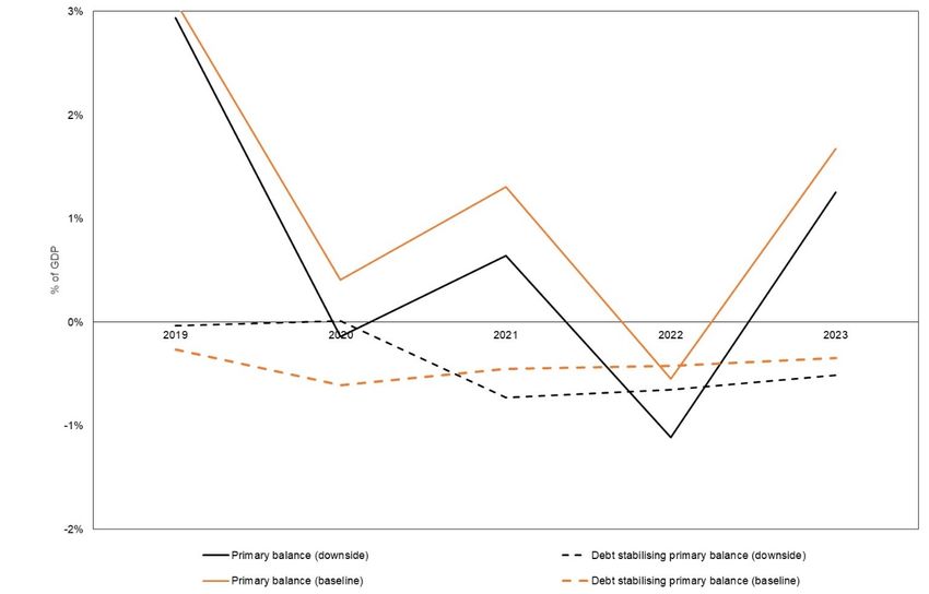
Table 3: Debt decomposition

 Public debt decomposition 2008 to 2018 (cumulative)

 Change in core Crown borrowings (gross debt) +13.7%

 Identified debt-creating flows (A+B+C) +13.0%

 Core Crown primary balance (A) +14.1%

 Automatic debt dynamics (B) -1.1%

 Contribution from interest rate/growth differential -1.2%

 Real interest rate +7.2%

 Real GDP growth -8.3%

 Contribution from real exchange rate depreciation 0.0%

 Other debt-creating flows (C) 0.0%

 Residual +0.7%

Source: The Treasury and author’s calculations

Gross public sector debt increased by approximately 13.7 percentage points between
2008 and 2018. The primary balance has the largest impact over this period, contributing
to a cumulative 14.1 percentage point increase in debt.

The automatic debt dynamics account for a small reduction in the debt ratio over this
period (1.1 percentage points). The growth-interest differential is small across this period,
which reflects not only low interest rates but also subdued growth. The contribution from
the real exchange rate depreciation was negligible across the period (a 0.05 percentage
point change if rounded to two decimal points) because the Government's holdings of
 11
foreign currency denominated debt was minimal. A small residual of 0.7% ensures that
the identity balances.

Figure 3 breaks the dynamics down into their year-on-year impacts. The annual change
in public debt is shown via the line graph and the bar graph disaggregates the effect of
each of the contributory factors. A positive item reflects an increase in the debt-to-GDP
ratio, while a negative item reflects a decrease in the debt-to-GDP ratio.

11 New Zealand’s Debt Management currently focus on New Zealand Dollar issuances in the domestic
 market. Foreign currency denominated issuances were paid down over the previous decade to nil. The
 2018/19 borrowing programme forecasts do not include any foreign currency debt issuances.

 W P 19/01 | Public D ebt D ynamics i n N ew Zeal and 13

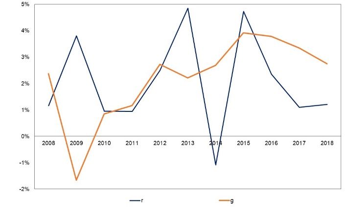
Figure 3: The debt dynamics

Source: The Treasury and author’s calculations

The gross debt ratio increased in the first half of the period and the largest increases
occurred in fiscal years 2009 and 2011, which is consistent with the effects of the GFC
and the Canterbury earthquakes. Figure 3 illustrates the relatively large primary balance
effect across this period. In 2009, the effects of the GFC are noticed. The primary deficit
accounts for the largest increase (approximately 7 percentage points of GDP). In 2011,
the net increase of approximately 8 percentage points is mainly attributed to the primary
deficit. From 2012 to 2018 gross debt-to-GDP either grows at a lower positive rate (2012
and 2015) or reduces.

Coefficient on the automatic debt dynamics

Figure 4 plots the coefficient on automatic debt dynamics (∅) and real interest ( ) and
growth ( ) rates for each year of the past decade. As set out in Section 2.1.3, a value of
∅ that is less than one implies favourable automatic debt dynamics. Our estimates for
the past decade show that, while close to the critical value of one, ∅ exceeded one for
multiple years. The effect of the interest-growth differential is the most unfavourable in
2009 due to negative real GDP growth.

Figure 4: Automatic debt dynamics (ø) Real interest and growth (r and g)

Source: Author’s calculations

 W P 19/01 | Public D ebt D ynamics i n N ew Zeal and 14

The estimated values for ∅ indicate relatively favourable automatic debt dynamics for
New Zealand since 2008.This reflects the low global interest rates that were experienced
in the post-GFC years. Interest rates on U.S. bonds have been and are still low, which
reflects the effects of the GFC and quantitative easing (Blanchard 2019). Declining global
real interest rates have affected public debt dynamics globally. New Zealand has
followed the global trend with declining ten-year bond rates on government debt, as
illustrated in Figure 5.

Figure 5: US Government and New Zealand Government nominal ten-year bond
rates

 8

 7

 6

 5
 Percent

 4

 3

 2

 1

 0
 1999Q1
 1999Q4
 2000Q3
 2001Q2
 2002Q1
 2002Q4
 2003Q3
 2004Q2
 2005Q1
 2005Q4
 2006Q3
 2007Q2
 2008Q1
 2008Q4
 2009Q3
 2010Q2
 2011Q1
 2011Q4
 2012Q3
 2013Q2
 2014Q1
 2014Q4
 2015Q3
 2016Q2
 2017Q1
 2017Q4
 2018Q3
 US 10-Year Bond Rate NZ 10-Year Bond Rate

Source: Federal Reserve Board, RBNZ, Haver

Debt stabilising primary balance

As a final measure of sustainability, Figure 6 plots the debt stabilising primary balance
and the actual primary balance across the period. We see that the primary balance
measure for 2009 to 2012 is below the debt stabilising primary balance, which coincides
with the increase in debt-to-GDP we observe over these years. From 2013 onwards, the
primary balance exceeds the debt stabilising primary balance in every year excluding
2015, which is consistent with the reduction in gross debt-to-GDP that we observe for
each year apart from 2015.

 W P 19/01 | Public D ebt D ynamics i n N ew Zeal and 15

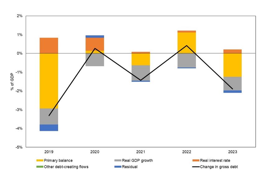
Figure 6: Primary balance & debt stabilising primary balance

Source: Author’s calculations

From 2008 to 2012, we observed an increase in the gross debt ratio. The increase is
attributable to the primary balance (deficit) effects of the GFC and the Canterbury
earthquakes. A more sustainable debt path emerges from 2013 to 2018, driven by the
primary balance (surpluses) and aided by the favourable automatic debt dynamics. This
is consistent with the Government's approach to building fiscal space in the post-GFC
years by decreasing expenditure-to-GDP and reducing debt. Declining global interest
rates, which reflect the effects of the GFC and quantitative easing, have led to favourable
automatic debt dynamics across the period (where < ) so the public debt burden
decreases, all else equal.

4 .2 The forecasts: 2019 to 2023
In this section we apply the Treasury's latest economic and fiscal forecasts (HYEFU 2018
at the time of writing) to the debt dynamics framework. The economic and fiscal forecasts
are included as exogenous inputs into the FSM and the debt dynamics framework.

HYEFU 2018 forecasts that the economy will expand at a pace that is close to its full
capacity, supported by population growth, government spending, accommodative
monetary policy and trading partner growth. Real GDP growth is expected to increase to
3.0 percent, on average, over 2019 and 2020, and is forecast to grow at a solid pace for
the remaining forecast years. The unemployment rate is projected to remain around 4.0
percent over the forecast horizon, below the Treasury’s estimate of the medium-term
sustainable rate. As growth picks up, continued labour market tightness is expected to
underpin a rise in wage growth and contribute to a sustained increase in inflation.
(HYEFU 2018). In line with the post-GFC years, interest rates are forecast to remain low.
In addition, primary surpluses are forecast for each year apart from 2022, partly driven
by an increase in tax-to-GDP over the 2018 HYEFU forecasts.

Over the five-year forecasts, and as a percentage of GDP, both the gross debt and net
debt ratio are expected to decline, as illustrated by Figure 7.

 W P 19/01 | Public D ebt D ynamics i n N ew Zeal and 16

Figure 7: Core Crown debt-to-GDP

 35%

 30%

 25%

 20%
 % of GDP

 15%

 10%

 5%

 0%
 2019 2020 2021 2022 2023
 Core Crown borrowings Net core Crown debt (excluding NZS Fund and advances)

Source: Author using data from the Treasury

Debt decomposition

Table 4 sets out the cumulative debt decomposition for the baseline HYEFU 2018
forecasts.

Table 4: Debt decomposition

 Public debt decomposition 2019 to 2023 (cumulative)
 Change in core Crown borrowings (gross debt) -8.1%

 Identified debt-creating flows (A+B+C) -8.0%

 Core Crown primary balance (A) -5.9%

 Automatic debt dynamics (B) -2.1%

 Contribution from interest rate/growth differential -2.1%

 Real interest rate +1.8%

 Real GDP growth -3.9%

 Contribution from real exchange rate depreciation N.A.

 Other debt-creating flows (C) 0.0%

 Residual 0.0%

Source: The Treasury and author’s calculations

We expect the gross debt ratio to decrease by 8.1 percentage points between 2019 and
2023. The primary balance amounts for the largest reduction of 5.9 percentage points.
The automatic debt dynamics contribute to a 2.1 percentage point reduction in the gross

 W P 19/01 | Public D ebt D ynamics i n N ew Zeal and 17

debt ratio as the growth-interest differential is forecast to be small, yet favourable. The
forecast dynamics are illustrated in Figure 8.

Figure 8: The debt dynamics

Source: The Treasury and author’s calculations

The gross debt ratio is projected to decline in each year excluding a small increase in
2022. The largest reductions are expected to occur in 2019 and 2023 and would be
driven by the forecast primary surpluses. The growth-interest differential is favourable
across the period.

Coefficient on the automatic debt dynamics

HYEFU 2018 forecasts low interest rates across the period. This is consistent with global
forecasts. In New Zealand, real GDP growth is forecast to increase in the first three years
of the period, underpinned by – among other things – low interest rates.

We estimate favourable values of ∅ for each year of the forecasts (i.e. values of less
than one). This means that, for each year < (Figure 9).

 W P 19/01 | Public D ebt D ynamics i n N ew Zeal and 18

Figure 9: Automatic debt dynamics (ø) Real interest and growth (r and g)

Source: Author’s calculations

Debt stabilising primary balance
Due to the favourable automatic debt dynamics, the debt stabilising primary balance is
negative across all the forecast years. The forecast primary balance exceeds the debt
stabilising primary balance in each forecast year excluding fiscal year 2022 when a
primary deficit is forecast. Smaller primary surpluses could (ceterus paribus) be run in
most years without destabilising debt.

Figure 10: Primary balance & debt stabilising primary balance

Source: Author’s calculations

Across the period, the gross debt ratio is expected to steadily decrease. Forecast primary
surpluses will have the most pronounced effect on the gross debt ratio, while the automatic
debt dynamics are forecast to be favourable and will thus enable further reduction.

The primary surplus is the main driver of New Zealand's forecast debt reduction over the
period (cumulatively 6 percent of GDP). Fiscal policy can affect real GDP growth via
aggregate demand in the short-term. The effect of the fiscal position on real growth has
been reflected in the HYEFU 2018 forecasts to the extent that it is accounted for in the
forecasting process.

 W P 19/01 | Public D ebt D ynamics i n N ew Zeal and 19

4 .3 The projections: 2024 to 2033
In the HYEFU 2018 FSM, most economic variables are at their trend growth rates by the
end of the forecasts. Real GDP growth is projected to between 2.1 percent and 2.3
percent across the projections. The long-term assumption for the unemployment rate is
4.3 percent, which is achieved in 2026, and the long-term government bond rate is
expected to reach a long-term stable rate of 5.3 percent by 2028.

After an initial decline, the Treasury projects gross and net debt levels to increase
incrementally for each year of the projections, though by 2032 the gross and net debt
ratios are still slightly lower than the 2023 ratios.

Figure 11: Core Crown debt-to-GDP
 30%

 25%

 20%
 % of GDP

 15%

 10%

 5%

 0%
 2024 2025 2026 2027 2028 2029 2030 2031 2032 2033
 Core Crown borrowings Net core Crown debt (excluding NZS Fund and advances)

Source: Author using data from the Treasury.

Debt decomposition

Table 5 sets out the cumulative debt decomposition for the baseline projections.

Table 5: Debt decomposition
 Public debt decomposition 2024 to 2033 (cumulative)
 Change in core Crown borrowings (gross debt) -0.6%
 Identified debt-creating flows (A+B+C) -0.6%
 Core Crown primary balance (A) -2.0%
 Automatic debt dynamics (B) +1.3%
 Contribution from interest rate/growth differential +1.3%
 Real interest rate +6.5%
 Real GDP growth -5.2%
 Contribution from real exchange rate depreciation N.A.
 Other debt-creating flows (C) 0.0%
 Residual 0.0%

Source: The Treasury and author’s calculations

 W P 19/01 | Public D ebt D ynamics i n N ew Zeal and 20

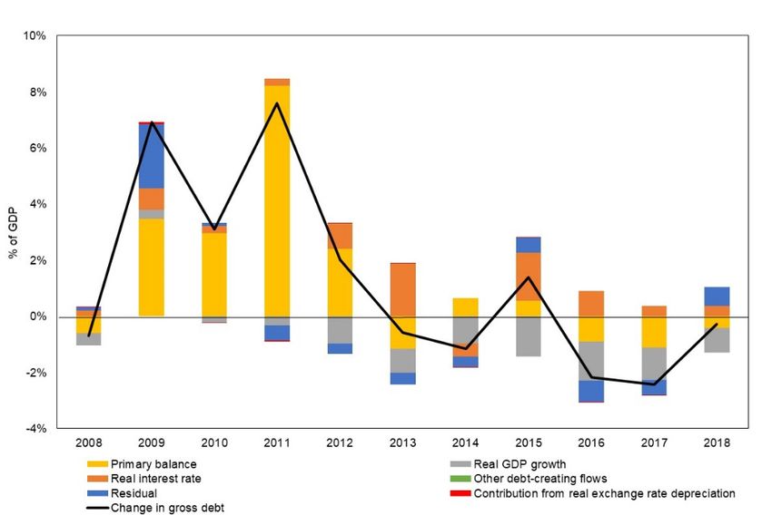
The level of gross debt is projected to decrease by a cumulative 0.6 percentage points
from 2024 to 2033. The primary balance is projected to contribute to a reduction of the
gross debt ratio of two percentage points, while the automatic debt dynamics are
expected to contribute to a small increase in the gross debt ratio (1.3 percentage points).

Figure 12: The debt dynamics

Source: The Treasury and author’s calculations

The Treasury projects the gross debt ratio to decrease each year until 2027. Debt
reduction is driven by (decreasing) primary surpluses for the first four years of the
projections, and this is supported by the favourable debt dynamics in the first three years
of projections. From 2027 onwards, small primary deficits and slightly unfavourable
automatic debt dynamics contribute to the projected increase in the gross debt ratio.

Coefficient on the automatic debt dynamics

Figure 13 shows ∅ is on an upward trend as real GDP growth remains within a band of
2.1 and 2.3 percent, and government bond rates converge to their long-run historical
average of 5.3 percent in nominal terms (real rate of 3.3 percent). From 2026 onwards,
the real borrowing rate is projected to be greater than real GDP growth, which means
that ∅ is greater than one. To keep debt on a sustainable track from 2026 – all other
things equal – primary surpluses will be required.

Figure 13: Automatic debt dynamics (ø) Real interest and growth (r and g)

Source: Author’s calculations

 W P 19/01 | Public D ebt D ynamics i n N ew Zeal and 21

Debt stabilising primary balance

In the context of unfavourable automatic debt dynamics from 2026, primary surpluses
will be required to stabilise debt-to-GDP. Figure 14 shows that the projected primary
balance falls below the projected debt stabilising balance from 2026. This supports the
increase in the debt ratio that we see from 2027.

Figure 14: Primary balance & debt stabilising primary balance

Source: Author’s calculations

Although the gross debt ratio is expected to be 0.6 percentage points lower by the end
of the projections, from 2027 onwards, deteriorating primary surpluses and increasingly
unfavourable automatic debt dynamics are reflected in the upward trend in the debt ratio.
Therefore, in order to stabilise debt, primary surpluses will be required from fiscal year
2026. Although the rate of increase in gross debt-to-GDP is small (0.3 percentage point
increase from 2027 onwards), there is a shift in the overall trajectory of debt to a path
that is less sustainable.

It is important to reinforce the uncertainty that underlies the projections. Economic and
fiscal variables converge to long-run average rates. However, in the case of interest
rates, history may not be a good guide. Blanchard (2019) finds that, although the gap
between interest rates and growth rates is expected to narrow, many forecasts and
market signals have interest rates remaining below growth rates for a long time. While it
is outside the scope of this paper to discuss the long-term history, we do find evidence
that low rates have persisted over recent years (see Figure 5). Whether rates will
continue to remain low or will return to levels consistent with long-term averages, is an
important question. If rates remain low, it would change the perspective on public debt
dynamics in New Zealand as it may alleviate concerns about public debt dynamics in the
projection period.

The projections also have characteristics that could make it more difficult to achieve
primary surpluses in projected years, when compared to the forecasts. Firstly, the
projections assume that tax-to-GDP stabilises, while no such constraints are placed on

 W P 19/01 | Public D ebt D ynamics i n N ew Zeal and 22

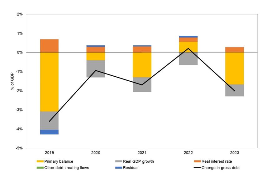
tax forecasts (tax-to-GDP increased by one percentage point of GDP over the 2018
HYEFU forecasts). Secondly, the projections account for an ageing population, and the
public pension expenses lift by around one quarter of a percentage point of GDP over
the forecast years, but by more than 1 percentage point of GDP over the projected years.
While these are technical assumptions, the flattening of tax-to-GDP in projections and
significant lift in public pension costs provide impediments over projections to attaining
primary surpluses that are either not present (flat tax to GDP) or less significant (the rise
of pension expenses) in forecasts.

4 .4 Scenario analysis
The Treasury prepares alternative forecast tracks that illustrate how the economy may
evolve if some of the main economic forecasts are altered. As a final measure, the debt
dynamics are analysed under an alternative forecast track. In the selected downside
scenario, which is from the HYEFU 2018 forecasts, declining trade volumes weigh
directly on global growth, lowering the demand for New Zealand exports, while weaker
sentiment lowers business investment, consumption, and global commodity prices. The
overall impact of the scenario sees GDP growth falling in nominal and real terms,
affecting tax revenue and the fiscal position. (New Zealand Treasury, 2018e)s

Figure 15: Core Crown debt to GDP
 35%

 30%

 25%

 20%
 % of GDP

 15%

 10%

 5%

 0%
 2019 2020 2021 2022 2023
 Core Crown borrowings Net core Crown debt (excluding NZS Fund and advances)

Source: Author using data from the Treasury.

Debt decomposition

Table 6 sets out the cumulative effect of the underlying drivers of gross debt under the
downside scenario, compared to the baseline scenario.

 W P 19/01 | Public D ebt D ynamics i n N ew Zeal and 23

Table 6: Debt decomposition

 Public debt decomposition (cumulative) 2019 to 2023 2019 to 2023
 Baseline Downside

 Change in core Crown borrowings (gross debt) -8.1% -6.0%

 Identified debt-creating flows (A+B+C) -8.0% -5.5%

 Core Crown primary balance (A) -5.9% -3.6%

 Automatic debt dynamics (B) -2.1% -1.9%

 Contribution from interest rate/growth differential -2.1% -1.9%

 Real interest rate 1.8% 1.9%

 Real GDP growth -3.9% -3.8%

 Contribution from real exchange rate depreciation N.A. N.A.

 Other debt-creating flows (C) 0.0% 0.0%

 Residual 0.0% 0.5%

Source: The Treasury and author’s calculations

The gross debt ratio is forecast to decrease by 6 percentage points under the downside
scenario. The automatic debt dynamics amount to a small reduction in gross debt (1.9
percentage points) as the growth-interest differential is forecast to be small, yet
favourable, across this alternative forecast horizon. The primary balance effect is less
under the downside scenario compared to the baseline, which reflects the weaker
forecast fiscal position.

Figure 16: The debt dynamics

Source: The Treasury and author’s calculations

Coefficient on the automatic debt dynamics

The effect of the automatic debt dynamics is small; however, it is projected to deteriorate
across the projection horizon and its effect on the accumulation of debt increases over
time. The value of this variable under the alternative scenario is less favourable in 2019

 W P 19/01 | Public D ebt D ynamics i n N ew Zeal and 24