QUALITY OF LIFE IN CHINESE CITIES - MUNICH PERSONAL REPEC ...

Munich Personal RePEc Archive

Quality of Life in Chinese Cities

Shi, Tie and Zhu, Wenzhang and Fu, Shihe

Xiamen University, Xiamen University, Xiamen University

12 January 2021

Online at https://mpra.ub.uni-muenchen.de/105266/
MPRA Paper No. 105266, posted 19 Feb 2021 06:32 UTC

Quality of Life in Chinese Cities

 Tie Shi
 E-mail: shitie@stu.xmu.edu.cn
 Wenzhang Zhu
 E-mail: zhuwenzhang029@163.com
 Shihe Fu
 E-mail: fushihe@xmu.edu.cn

 Wang Yanan Institute for Studies in Economics
 Xiamen University

 January 10, 2021

Abstract: The Rosen-Roback spatial equilibrium theory states that cross-city variations
in wages and housing prices reflect urban residents’ willingness to pay for urban
amenities or quality of life. This paper is the first to quantify and rank the quality of life
in Chinese cities based on the Rosen-Roback model. Using the 2005 1% Population
Intercensus Survey data, we estimate the wage and housing hedonic models. The
coefficients of urban amenity variables in both hedonic models are considered the
implicit prices of amenities and are used as the weights to compute the quality of life for
each prefecture city in China. In general, provincial capital cities and cities with nice
weather, convenient transportation, and better public services have a higher quality of
life. We also find that urban quality of life is positively associated with the subjective
well-being of urban residents.

Key words: Spatial equilibrium, hedonic model, urban amenity, quality of life, life
satisfaction

JEL Codes: H44, J31, J61, R13, R23, R31

Acknowledgement: We thank Shi Li, Xuewen Li, Shimeng Liu, Minjun Shi, and
participants of the 4th China Labor Economics Forum for very helpful comments. Shihe
Fu acknowledges financial support by the National Natural Science Foundation of
China (Grant # 71773096 and Basic Scientific Center Project 71988101).

 1

1 Introduction

Quality of life refers to “the satisfaction that a person receives from surrounding human
and physical conditions” (Mulligan et al., 2004). Different from individual satisfaction
derived from private consumption, quality of life reflects people’s value for “social
goods”—quasi-market and non-market goods (Wingo, 1973). It is considered an
economic good and varies largely across locations (Wingo, 1973; Gillingham and
Reece, 1979). Urban amenities, which are location-specific goods and services that
make cities attractive for living and working, are the primary determinants of quality of
life in cities (Rosen, 1979; Diamond and Tolley, 1982). Urban amenities can be natural
(nice weather, good air quality), human-made (museums, restaurants, public services),
or social (tolerant social milieu, safety); they can also be utility generating to
households (consumption amenities) or productive to firms.

Quality of life in cities affects directly not only individual well-being, but also location
choices of households and firms and urban growth (Mulligan et al., 2004; Shapiro,
2006; Mulligan and Carruthers, 2011). Taken American cities as an example, cities with
rich consumption amenities and nice weather also have high population density and
high growth in population, employment, and housing value and rents (Rappaport, 2007,
2008; Carlino and Saiz, 2019). With persistent income growth and rapid urbanization in
China during the past few decades, people migrate not only for better job opportunities
but also for better public services, consumption amenities, and environmental qualities
in cities (Xing and Zhang, 2017). The general public and policy makers have been
paying increasing attention to urban quality of life in China.

Surprisingly, to the best of our knowledge, so far there is no rigorous study that
quantifies and ranks urban quality of life in China. A few available rankings either used
survey data by asking people’s subjective ranking via phone interviews or internet
questionnaires or calculate a quality of life index by weighted sum of a set of indicators
measuring different urban amenities where the selection of indicators and weights is
arbitrary and not grounded in economic theory. The rankings of some cities are often
counter-intuitive and inconsistent with the consensus in the popular press. For example,
The Report on Quality of Life in 35 Cities in China, released by the Research Center for
Urban Quality of Life (RCUQL) at Capital University of Economics and Business,
ranked Xiamen 29 among the 35 cities in 2017, while it is often ranked among the top
in the popular press.1

In contrast, many empirical studies have estimated the quality of life in cities of many
other countries, including Canada (Giannias,1998; Albouy et al., 2013), England
(Srinivasan and Stewart, 2004), Russia (Berger et al., 2008), Germany (Buettner and
Ebertz, 2009), Itlay (Colombo et al., 2014), and notably the USA (Rosen, 1979;
Roback, 1982; Kahn; 1995; Gabriel et al., 2003; Rappaport, 2007, 2008, 2009; Winters,

1
 The report is published in a Chinese journal “Economic Perspectives,” 2017, no.9, 4-19.
 2

2013; Albouy et al., 2016). These studies are well grounded in the commonly accepted
theory of spatial equilibrium developed by Rosen (1979) and Roback (1982).

The Rosen-Roback spatial equilibrium model states that with free mobility,
compensating differentials in wages and housing prices (rents) across cities reflect
people’s willingness to pay for urban amenities or quality of life in cities to achieve the
spatial equilibrium under which utility are equalized across cities. To put it another way,
people are willing to pay higher housing prices or rents, or are willing to accept lower
wages, to live in cities with better amenities. By estimating a wage hedonic model and a
housing hedonic model including both individual (worker or housing unit) attributes and
city amenity variables, we can use the coefficients of amenities as their implicit prices.
The quality of life index for a city can then be calculated by the weighted sum of
amenity quantities in that city, where the weights are the implicit prices. This approach,
well grounded in the Rosen-Roback model, has been the standard application in the
empirical literature on evaluating quality of life in cities (Gyourko et al., 1999; Lambiri
et al., 2007).

The purpose of this paper is to apply the Rosen-Roback framework and hedonic models
to quantify the quality of life in Chinese cities. We use the 2005 1% Population
Intercensus Survey data, the only available micro dataset so far with both labor income
and housing costs information for all cities in China, and city amenity data to estimate
compensating differentials in wages and housing prices and rents for 287 prefecture
level cities. We then compute and rank the quality of life index for these cities.
Following Blomquist (2006), we select three types of amenities: climate, environmental
quality, and urban conditions (city characteristics). We find that quality of life varies
tremendously across cities. In general, cities with a high quality of index are provincial
capital cities or cities with nice weather, convenient transportation, or good medical and
educational public services. The quality of life index is positively associated with the
self-reported subject well-being of urban residents, suggesting that urban quality of life
indeed to some degree measures happiness in cities. Not surprisingly, our ranking of
quality of life in cities is very different from those not based on economic theory.

Our findings have important public policy implications for city governments. As human
capital is crucial for urban growth (Simon, 1998), many city governments in China have
been striving to attract high-skilled workers but their policies are rather simple and
narrow. The main policies are relaxing residence (Hukou) restrictions and offering
lump-sum housing or relocation subsidies (Zhang et al., 2019). Since high-skilled
workers have a higher willingness to pay for urban amenities, our study suggests that
local governments can attract talents by improving city amenities, particularly
educational and medical public services, transportation and commuting, and
environmental qualities.

The next section introduces briefly the intuition of the Rosen-Roback spatial
equilibrium model and outlines the steps for empirical implementation. Section 3

 3

describes the data and Section 4 specifies the empirical models. Section 5 presents our
evaluation and ranking of quality of life in Chinese cities and Section 6 concludes.

2 The Rosen-Roback model and urban quality of life

Rosen (1979) developed a theoretical framework to estimate a wage-based index of
urban quality of life where the implicit price weights for urban consumption amenities
are estimated from a wage hedonic model including both individual worker attributes
and urban amenity variables. Roback (1982) extended Rosen’s model by incorporating
further housing markets and productive amenities. The model has a set of standard
assumptions: Households have the identical preference and derive utility from a
composite consumption good, housing services, and location-specific amenities. Each
household supplies one unit of homogenous labor and wage is the only income source.
Workers can move freely across cities. For a given city j, the indirect utility function of
a representative household can be written as

 = ( , ; ), (1)

where indicates the highest utility level that households can achieve given wage level
 , housing rent , and a vector of urban amenities with elements .2 Higher

wage increases utility ( > 0, where “∂” denotes partial derivative) and higher rent
 
reduces utility ( < 0), ceteris paribus. The sign of is positive if is an
 
amenity (for example, fresh air or cool summer) and negative if it is a disamenity (say,
congestion or crime).

Firms are assumed to have the identical, constant-returns-to-scale technology with
capital, labor, and land as the inputs to produce the composite consumption good.
Capital is freely mobile and the composite good is tradable in a nationwide, competitive
market whose price is normalized to be one. To ease the notations and to simplify the
analysis, we further assume that the land rents paid by the firms are the same as the
housing rents by households.3 The unit cost function of firms located in city j is given
as follows:

2
 We use housing rent in equation (1); alternatively, we can use housing price. Since housing price is the
present value of future housing rents flow, we use housing price and rents interchangeably in this paper.
3
 It is consistent to assume that households “consume” land. This requires land rents or land prices data
be used in the empirical part as in Roback (1982). However, households consume housing services and
housing price or housing rents data can also be used to estimate the implicit prices of amenities. This
approach is commonly used in the recent literature (Blomquist, 2006) and we follow suit in this study.
 4

 = ( , ; ), (2)

where denotes the lowest cost of producing one unit of output by firms given wage
level , land rent , and urban amenities . High input prices increase unit cost:
 
 > 0 and > 0. Similarly, the sign of depends on whether the specific
 
amenity is productive to firms or not. For example, being located along a navigable

river or in coastal area can reduce transport costs of shipping inputs and outputs while
clean air increases production cost as firms need to install equipment to reduce
emissions of air pollutants.

The equilibrium of the model requires no spatial arbitrage meaning that in the spatial
equilibrium both households and firms are indifferent between which city to locate:
utility levels are equalized across cities (equilibrium utility level is denoted by ̅) ; so
are unit costs.4 This can be stated by the following conditions:

 ̅ = ( , ; ); (3)

 1 = ( , ; ). (4)

The intuition of the spatial equilibrium with urban amenities can be demonstrated by
Figure 1. The horizontal axis denotes wages in different cities; the vertical axis, rents.
The iso-utility curve is upward sloping, meaning that for a given distribution of
amenities across cities, 0 , workers need to receive higher wages in cities with higher
rents so that utility levels can be equalized across cities. Similarly, the iso-cost curve is
downward sloping: for a given spatial distribution of amenities, firms are willing to pay
higher rents with in cities with lower wages, or higher wages in cities with lower rents
to maintain the same unit cost across cities. The intersection of the two curves
determines the equilibrium wage and rent.

 (Insert Figure 1 here)

Figure 1 can also be used to show the comparative static analysis. For example, if some
amenities are improved in all cities ( 1 > 0 ), then the iso-utility curve will move
upward from ( , ; 0 ) to ( , ; 1 ) because now for a given wage level workers
are willing to pay even higher rents to enjoy better amenities (or for given rents workers
are now willing to accept lower wages). The story would end here if the improved
amenities do not affect firm productivity. However, if they enhance firm productivity,
by the same token, the iso-cost curve will shift up because now for a given wage level

4 Given the production technology has constant returns to scale and the output price is normalized to be
one, the unit cost equals one in the competitive equilibrium.
 5

firms are willing to pay higher rents to benefit from the more productive amenities. In
the new spatial equilibrium, equilibrium rent will be higher but the equilibrium wage
can be higher or lower depending on the degree of shift of the iso-cost curve. This has a
very important implication: in the wage hedonic regression the effect of an urban
amenity can be positive or negative depending on how productive the amenity is to
firms.

The variations in housing rents and wages across cities reflect households’ willingness
to pay for local amenities or quality of life. The monetary value or the implicit prices of
local amenities can be derived from these compensating differentials in wages and rents.
Taking total differentials with respect to both sides of equations (3) and using the Roy’s
identity, we can derive equation (5) as follows:

 = ⁄ =ℎ⋅ − , (5)
 
where and denote the compensating differentials in rent and wage due to a
 
small change in a particular amenity around the spatial equilibrium, h is the optimal
housing consumption of a representative household. The sum of both compensating
differentials in rent and wage is the monetary value of the amenity and is defined as the
implicit price of amenity, . Note that the sign of the implicit price is indeterministic.
A negative sign means that households need to be subsidized or compensated to bear
the disamenity (say air pollution or very cold winter).

The compensating differential in rent ( ) and in wage ( ) can be estimated from a
 
housing hedonic model and a wage hedonic model with urban amenity variables
included. Then, the implicit price can be calculated based on equation (5). The
quality of life (QOL) index for city j is the weighted sum of all amenities in city j where
the weights are the implicit prices of amenities:

 = ∑ . (6)
 
This QOL index can be considered a household’s willingness to pay for amenities in
city j and can also be used to rank cities in terms of quality of life.

Two caveats are worth noting before we proceed to the empirical part. First, since the
publication of Rosen (1979) and Roback (1982), the spatial equilibrium framework has
been extended in different directions. For example, Blomquist et al. (1988) incorporate
agglomeration economies; Gyourko and Tracy (1991) consider the effect of local
taxation on quality of life; Graves and Waldman (1991) focus on retirees’ preference
toward urban quality of life; Gabriel and Rosenthal (2004) and Chen and Rosenthal
 6

(2008) extend the framework to evaluate business environment of cities; Albouy and
Lue (2015) allow for commute cost. Our goal in this paper is rather modest: we focus on
only quality of life from the perspective of average households and consider only a set
of commonly studied amenities.

Second, does the spatial equilibrium framework apply to China? Our simple answer is
yes. There are two main reasons. First, the spatial equilibrium mechanism applies to any
allocation in space to reduce arbitrage across locations as long as factors can move
across locations. Although moving goods and people across cities is costly, this does not
prevent spatial allocation from converging to the spatial equilibrium as long as
economic agents seek to maximize utility or profits so that any spatial arbitrage
opportunities will be fully explored eventually. Second, some empirical evidence
supports the existence of spatial equilibrium. Greenwood et al. (1991) conclude that the
American regional economies (at the state level) during 1971~1988 are not in
disequilibrium by comparing the income in equilibrium and actual income. Berger et al.
(2008) find that compensating differentials exist in both the planned economy regime
and the transition period in Russia. Chauvin et al. (2017) argue that no evidence shows
that the spatial equilibrium hypothesis does not hold in China and Brazil. Although it is
well known that rural-urban and inter-city migration barriers exist in China, notably the
residence regulation (Hukou system), the massive rural-urban migration and rapid
urbanization during the past few decades do suggest that inter-regional labor mobility is
relatively high. It is not unreasonable to apply the spatial equilibrium framework to
evaluate urban quality of life in China.

3. Data

3.1 Main dataset

Estimating the implicit prices for urban amenities based on the Rosen-Roback
framework requires not only data for urban amenities, but also a sample of individual
workers with demographic and income variables and a sample of individual housing
units with housing price (rent) and housing attributes variables for each city. The only
such a dataset available in China that meets these requirements, to the best of our
knowledge, is the 2005 1% Population Intercensus Survey (sometimes also called the
2005 minicensus), provided by the State Statistical Bureau of China. A few nationally
representative household survey datasets with rich demographic information are
available in China for recent years, such as the China Family Panel Survey, China
Household Finance Survey, China Household Income Project Survey, but the number of
households in each city is small and city identity is not publicly released without special
request and approval. City governments host and maintain housing transaction data and
a few large real estate brokers also collect housing transaction data for many cities, but
we are unable to access these data. The dataset we are using is a bit outdated but it
enables us to conduct the first evaluation of urban quality of life in China.

 7

Our sample includes 287 prefecture level cities because for the purpose of this study,
the selected urban amenity variables are available only for these cities. Below we
describe the variable definitions and other data sources.

3.2 Housing and wage

The 2005 1% Population Intercensus Survey data provide information on “costs of
purchasing or building a housing unit” for each home owner. We exclude those housing
units built by households themselves and use “costs of purchasing a housing unit” as the
proxy for housing price because it closely reflects the transaction price. We winsorize
housing price at the top and bottom 1%. Housing attributes variables include structure,
number of floors, building age, number of rooms, floor area, whether the unit has a
kitchen, bathroom, tap water, cooking fuel, and full or partial ownership. Detailed
location information of a housing unit in a city is not available. To control for
unobserved neighborhood attributes of housing units, we assign each housing unit into a
group with homogenous attributes in terms of structure, floor, building age, and floor
area (see Table A1 in the Appendix) and add group fixed effects to the housing hedonic
model. The rationale is that observationally identical individuals are very likely to have
similar unobservables (Bayer and Ross, 2006; Altonji and Mansfield, 2018; Oster,
2019). 5

The data also provide “monthly rental payment” information and we use this to measure
housing rent. Rental markets are not well developed in Chinese cities given the very
high home ownership in urban China.6 Many rental units are in “urban villages”
accommodating rural migrants (Song et al., 2008) and the rental data may be noisy.
Since housing price is the present value of future rents cash flow, we also estimate the
housing rent hedonic model as a robustness check for implicit prices of amenities but
evaluate urban quality of life based on only housing price hedonic model.

We select workers of prime-age (16~65 for males and 16~60 for females) who are
employed or have a job. Wage is measured by monthly labor income calculated from
the data and is also winsorized at the top and bottom 1%. Individual demographic
variables include gender, age, education, marital status, ethnicity, self-employed or not,
and occupation (see Appendix Table A2). To control for unobserved individual abilities
that could affect income, we also assign each worker into a homogenous group in terms
of the main demographic traits and include these group fixed effects in the wage
hedonic model.

3.3 Urban amenities

5
 Housing hedonic models in the literature of urban quality of life generally do not consider
neighborhood attributes. In our study, including these group fixed effects generates similar results to the
model without group fixed effects.
6
 The home ownership rate is 81.26% in 2005 urban China. Web source (in Chinese):
http://www.stats.gov.cn/tjsj/tjgb/qttjgb/qgqttjgb/200607/t20060704_30621.html.
 8

Following Blomquist (2006), we select three types of urban amenities: climate,
environmental quality, and urban conditions (city attributes), to capture the main aspects
of urban quality of life. We admit that our selection is a bit subjective. Given there are
dozens of or even hundreds of amenity variables, a more sophisticated selection criteria
may involve new techniques such as machine learning or high-dimensional
econometrics. We leave this extension for future research.

3.3.1 Climate variables

We select three variables to measure a city’s climate characteristics: monthly
precipitation, average daily sunshine duration (hours), and temperature. These data are
directly from China Meteorological Data Service Center. Instead of using the raw
temperature data, we follow Zheng et al. (2009) and construct a city temperature index
to measure the degree of comfortableness in terms of temperature based on the
maximum and minimum temperature of each city in 2005:

 2 ℎ ℎ 2
Temperature index = √( 
 
 − ) + ( ℎ ℎ − ) , (7)

where and ℎ ℎ are the annual minimum and maximum
 and
temperature of each city in our sample, respectively. ℎ ℎ 
 
are the maximum of and the minimum of ℎ ℎ in the sample of
287 cities, measuring comfortable temperature (e.g., warm winter and cool summer).
This index quantifies the degree of comfortableness in terms of a city’s temperature; the
smaller the value, the more comfortable the city’s temperature is.

3.3.2 Environmental quality variables

We construct three variables to measure urban environmental quality: annual mean
concentration of PM2.5, coastal location, and green coverage ratio. Annual mean
concentration of PM2.5 are derived using the GIS software from the grid level data
provided by the Atmospheric Composition Analysis Group at Dalhousie University,
Canada.7 We create a dummy variable “costal city” to indicate whether a city is located
in the coastal area based on the coastal city list specified in China Ocean Yearbook
2006. Coastal cities have location and transport advantage but also have nice beach
view and better environmental quality. Green coverage ratio is the ratio of greened land
area to the total built land area of a city and the data are from China Urban Statistical
Yearbook 2006.

3.3.3 Urban condition variables

7
 The web link is http://fizz.phys.dal.ca/~atmos/martin/?page_id=140. The State Environmental
Protection Administration of China publishes daily air pollution index including PM10 concentration in
2005 but only for 72 cities; PM2.5 data become available only since 2013.
 9

Numerous city attributes or urban condition variables are available and there is no
consensus which set of variables should be used to measure quality of life. Following
the literature, we select a set of variables to measure urban public services,
transportation as well as city sizes. The data are also from China Urban Statistical
Yearbook 2006.

City size is measured by both population density and population size. Large cities
generate strong agglomeration economies and knowledge spillovers and thus improve
quality of life (Glaeser, 1999; Rotemberg and Saloner, 2000; Duranton and Puga, 2004)
but may also reduce social trust and increase social and occupational segregation
(Benabou, 1993; Glaeser, 1998). Following the literature (Colombo et al., 2014), we
consider population density an amenity but keep population size as a control variable to
avoid ranking bias toward large cities.

The number of theatres per one hundred thousand population in a city is used to
measure the cultural and entertainment amenities. The number of hospital beds per ten
thousand population in a city measures the availability of medical services. Public
education quality is measured by the teacher-student ratio in high schools and the
number of higher education institutions (colleges and universities). Transportation
accessibility is measured by road area ratio (total road area divided by total urban area)
and the number of airline routes, reflecting intra- and inter-city mobility. Given the
important role of urban hierarchy in China (Chan and Zhao, 2002; Li, 2011; Bo, 2020;
Jia et al., 2021), we also create a dummy variable “capital city” set to be one if a city is
a provincial capital, a sub-provincial city, or is directly under the central government.

Many empirical studies include unemployment rate and crime rate to measure social
amenities (Roback, 1982; Blomquist, 2006). These are very important urban conditions
and factors that affect location choice of households and businesses. Unfortunately, the
data for these variables are not publicly available for Chinese cities.8 We also
deliberately omit some important amenity variables to avoid high collinearity with the
selected variables such as concentration of other air pollutants, highway mileage or
railway length.

The summary statistics of the key variables in estimation are reported in Table 1.

 (Insert Table 1 here)

4 Model specification

The implicit prices of urban amenities can be obtained from the housing price and wage
hedonic regression models:

8
 Unemployment rate data based on registered unemployment are available but underestimate actual
unemployment rate and also lack variation across cities.
 10

ln ℎ = 0 + 1 ℎ + 2 + ℎ ; (8)
 ln = 0 + 1 + 2 + . (9)

The dependent variable in the housing hedonic regression is ln ℎ , the logarithm of
price of housing unit h located in city ; we also estimate the housing hedonic model
using monthly rent. ℎ is the vector of housing attributes as listed in Table A1. is
the vector of urban amenity variables for city j and the full list is presented in Table 1.

In the wage hedonic model, is the monthly income of worker k who is located in
city j; is the vector of individual demographic traits and the full list is presented in
Table A2. ℎ and are error terms. The estimated coefficient vector 2 and 2
are the marginal effects of urban amenities on housing price and wage, respectively,
 
corresponding to and in equation (5).9
 
The premise of estimating the implicit prices of urban amenities from these hedonic
models is that after controlling for individual housing attributes and individual worker
attributes, there are no individual unobservables that correlate with urban amenity
variables. This is unlikely due to spatial sorting based on individual unobserbables. For
example, high ability workers prefer living in cities with rich amenities. Our remedy is
to include a large set of group fixed effects as described in the Data section under the
rationale that individuals who belong to the same group are likely to have similar
unobservables.

We estimate Models (8) and (9) using the ordinary least squares method. The samples
include 421,660 housing units and 1,157,385 workers. To allow for the possible spatial
correlation within a city, we cluster the standard errors at the city level.

To calculate a household’s annual willingness to pay for an urban amenity using
equation (5), we also need to have data for the number of working adults in and the
annual housing expenditure by a representative household.10 To simplify the
calculation, we impute these data only for a “nationally” representative household. The
labor force participation rates of men and women in 2005 are 77.5% and 64.3%,
respectively, based on the 2005 1% Population Intercensus Survey. If we assume that an
employed male household member represents one full-time worker, then an employed
female household member can be considered equivalently 0.83 full-time worker.
Assuming a representative household has a working couple, this means 1.83 effective
full-time wage earners. The monthly income is 625 CNY in Table 1. Therefore, the
annual wage compensating differential for a representative household for a particular
amenity i is CNY− 2 × 1.83 × 625 × 12. Note here we add a negative sign because a
negative value of 2 in the wage model means that the household is willing to accept a

9
 Strictly speaking, 2 corresponds to . We slightly abuse the notations here.
 
10
 The housing hedonic model implies that = 2 or = 2 ; this also implies that
 
 = 2 assuming = where r is the annual housing rents and i is the constant, annual
 
capitalization rate.
 11

lower wage for that amenity, or put it in another way, willing to pay more for that
amenity.

Imputing monthly housing expenditure is tricky. Monthly rental payment in our data is
ready for use but is very likely noisy and underestimated given the under-developed
rental markets and many “urban villages” in cities. Imputing the capitalization rate for
housing market involves more parameters such as growth rate of rents. We decide to use
the monthly mortgage payment for a typical long-term mortgage transaction in 2005.
Based on the Report on China’s Monetary Policy Implementation for the first quarter of
2005, released by the People’s Bank of China (also the central bank of China), in a
sample of 10 cities surveyed, the average borrowing term is 17 years with the average
down payment ratio of 37% and long-term interest rate of 6%. Given the mean housing
price of CNY74,010 in Table 1, the monthly mortgage payment is CNY365, which is
higher than the mean monthly rental payment of CNY261 in Table 1.11 The annual
compensating differential in housing price or housing expenditure for a particular
amenity is CNY 2 × 365 × 12. Adding up the compensating differentials in both
housing price and wages, we can compute the implicit price for amenity . The
quality of life index for each city can then be calculated using equation (6).

5. Results

5.1 Implicit prices for urban amenities

Table 2 reports the results of estimating Models (8) and (9) where the coefficients of
individual attributes are suppressed. Column (1) is the housing price hedonic model.
The coefficients of amenity variables are jointly statistically significant (F= 35.7).
Including amenity variables improves the model fitting by about 3.2% in terms of
change in R-squared. Of the amenity variables with statistically significant coefficients,
we can see that households are willing to pay a higher housing price for more sun
shining days, coastal location, cultural facilities such as theatres, convenient inter-city
transportation (more airline routes), and for higher urban hierarchy status (provincial
capital). These findings are intuitive and consistent with life experience in reality. For
the coefficients insignificant, many of them have the expected sign, for example, people
are willing to pay a higher housing price for better medical and education services. The
coefficient of PM2.5 concentration is insignificant possibly because households are not
well aware of air pollution problem back in 2005. Not until 2013 did the public become
alert to air pollution when “smog” caught the public attention (Zhang et al., 2019).
Another possible interpretation of insignificant coefficients is that some amenities are
not fully capitalized into housing values (and wages) in the transition economy due to

11
 This also implies an annual capitalization rate of 5.92%, which is in the range of between 4.35% and
7.85% used in other empirical studies (Blomquist et al., 1988; Berger et al., 2008).

 12

institutional barriers to inter-city mobility. Column (2) uses housing rent as the
dependent variable and the pattern of the results is very similar.

 (Insert Table 2 here)

Column (3) presents the wage hedonic model results. Including amenity variables
improves the model fitting by about 2.7% and most of the coefficients are significant.
The sign of a coefficient in the wage hedonic model is worth noting. If an amenity does
not affect firm productivity but improves household utility, then households are willing
to sacrifice some wage compensation to enjoy more of the amenity. In this case the
coefficient of this amenity in the wage model should be negative. However, if an
amenity enhances firm productivity, firms then will be willing to pay higher wages for
given rents (referring to Figure 1), which could more than offset households’
willingness to sacrifice, resulting in a positive coefficient. Column (3) suggests that
most of the amenities are also productive.

Table 3 shows how the implicit price of each type of amenity is calculated based on the
results in Table 2. Column (1) calculate the housing price compensating differential—
by how much more annual housing expenditure households are willing to trade for a
marginal increase in a particular type of amenity. It equals the monthly housing
expenditure (CNY365) multiplied by the coefficient in Column (1) of Table 2 ( 2) and
then multiplied by 12 months. For example, households are willing to pay CNY 245.28
more on housing expenditure each year to enjoy one more hour sunshine every day and
CNY 779.64 more on housing expenditure to live in a coastal city. The negative sign
means that households are willing to pay less on housing to live with that disamenity.
For example, to attract households to a city with temperature index ten unit higher,
annul local housing rents must be CNY43.8 lower.

 (Insert Table 3 here)

Column (2) of Table 3 calculates the wage compensating differential—by how much
annual income households are willing to give up to enjoy a particular amenity. It equals
the average monthly household income (CNY625.2×1.83) multiplied by the coefficient
in Column (3) of Table 2 ( 2) and then multiplied by 12 months. Note that in Column
(2) of Table 3 we also add a negative sign to this number so that a positive wage
compensating differential means that households are willing to pay more (by means of
accepting a lower wage) to enjoy that consumption amenity while a negative number
means that households are willing to pay less (by means of demanding for higher wage
compensation) to live with the disamenity. For example, households require
CNY1035.34 more annual income to live in coastal cities; this is likely due to much
higher firm productivity and firms’ higher willingness to pay for workers in coastal
cities.

Column (3) reports the implicit price of each amenity ( in Equation (3)) which is the
sum of compensating differentials in housing expenditure and wage, reflecting a
 13

representative household’s total willingness to pay for each amenity in 2005. A negative
number in Column (3) can be understood as the compensation or subsidy that a
household requires. Overall households are willing to pay more to live in a capital city
and cities with high population density, to enjoy more sunshine, better cultural and
medical public services, and more convenient transportations.

5.2 Ranking cities by quality of life index

Using the implicit prices for amenities computed in Table 3 as the weights and equation
(6), we can calculate the quality of life index for 287 cities in our sample. It is a
household’s aggregate willingness to pay for living a city with a particular set of urban
amenities. The larger the QOL index, the higher the quality of life in that city. To
facilitate comparison, we standardize the QOL index for each city by subtracting the
mean value of the QOL index in the sample. A positive number means households are
willing to pay more for living in a city with better than average amenities and vice
versa. The top and bottom 20 cities in terms of QOL are listed in Table 4 and the full
list is in Table A4.

The four first-tier cities, Shanghai, Beijing, Guangzhou, and Shenzhen are ranked
among the top 5 highest quality of life; Xiamen, a coastal city best known as “the
“Garden of the Sea”, where the authors are currently (and luckily) living, is ranked the
9th. Most of the top 20 cities are also provincial capital cities. The ranking of the top 20
cities is roughly consistent with the informal rating in the air or from the popular press.
The bottom 20 cities are in general small and medium size cities located all around the
country.

 (Insert Table 4 here)

We also decompose the QOL index into three components: climate, environmental
quality, and urban conditions. Their correlation coefficients are presented in Table 5.
Notably, urban condition index is highly correlated with the overall QOL index
(correlation coefficient is 0.96), suggesting that accessibility and quality of public
services, transportation, and political status of a city are the most important
determinants of QOL. Climate amenities are also important (correlation coefficient is
0.24). Surprisingly, environmental quality index is not correlated with the overall QOL
index (correlation coefficient is 0.03 and insignificant), possibly because people are not
well aware of the environmental issues fifteen years ago; it is negatively correlated with
urban condition index, implying that urban development is coupled with agglomeration
diseconomies such as environmental pollution.

 (Insert Table 5 here)

5.3 Urban quality of life and subjective well-being

 14

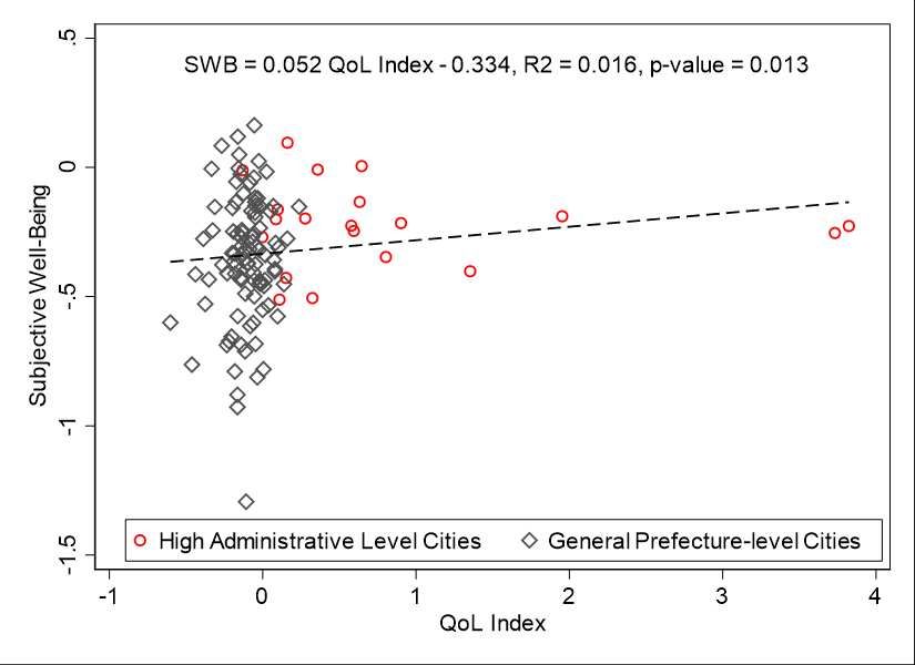
Whether cities can make people happy has attracted much attention. Many studies use
residents’ self-reported life satisfaction or subjective well-being (SWB) to measure
happiness and connect this with urban amenities such as air quality, climate, and urban
growth (Luechinger, 2009; Ferreira and Moro, 2010; Glaeser et al., 2016). Moro et al.
(2008) use subjective well-being data to rank quality of life in counties in Ireland.
Oswald and Wu (2010) find that in the USA the state-level life satisfactions adjusted by
demographic traits are highly correlated with the QOL ranking estimated by Gabriel et
al. (2003), with a correlation coefficient of 0.6, suggesting that self-reported subject
well-being does correlate with locational amenities. In this subsection, we also attempt
to test whether our ranking of QOL in cities is highly correlated with the subject well-
being reported by urban residents.

We use the 2010 China Family Panel Survey because its questionnaire asks
interviewees to rate their degree of happiness.12 The question asks “How much do you
feel happy?” with optional answers “very unhappy”, “unhappy”, “okay”, “happy”, “very
happy” that are coded as the integers between 1 and 5. Following Oswald and Wu
(2010)’s approach, we first regress individual reported happiness ratings on city dummy
variables and a set of individual demographic traits including gender, age, ethnicity,
education, marital status, and working status. The coefficient of each city dummy
variable is treated as the subjective well-being of that city.

Assuming QOL change only smoothly from 2005 and 2010, we can correlate 2010
SWB of cities and 2005 QOL indexes in cities. Column (1) of Table 6 regresses the
SWB on the overall QOL indexes across cities and the coefficient is positive and
statistically significant at the 5% level, suggesting positive association between
subjective well-being and quality of life in cities. This is also demonstrated in the scatter
plot with a fitted line in Figure 2. The other columns in Table 6 show that SWB is
positively correlated with the QOL indexes in terms of climate and urban conditions but
not environmental quality. Figure 3 also shows the statistically significant negative
correlation between city level SWB and our ranking of the same cities based on the
QOL index; that is, the cities in the top list of QOL are also happier.13

12 The CFPS is a nationally representative survey of Chinese households and focuses on both economic
and non-economic well-being of each household member. It is conducted by the Institute of Social
Science Survey at Peking University every other year since 2010. It uses a multistage, probability
proportional to size sampling method with implicit stratification to better represent Chinese population.
The 2010 baseline sample covers 25 provinces and 118 prefecture level cities. The official web site is
http://www.isss.pku.edu.cn/cfps/en/index.htm.
13 Note that the R2’s in Table 6 and Figures 2-3 are very small compared with 0.36 in Oswald and Wu
(2010). This is probably because our city-level SWB is less precisely estimated due to the much smaller
number of workers in each city in the CFPS data (on average about 300 workers per city) while Oswald
and Wu (2010) used the data with 1.3 million people in the 50 states in the USA.

 15

(Insert Table 6 here)

 (Insert Figure 2 here)
 (Insert Figure 3 here)

5.4 Comparison of QOL rankings

The Research Center for Urban Quality of Life at Capital University of Economics and
Business started publishing QOL report for 35 large and medium size cities since
2011.14 The RCUQL constructs two indexes to rank cities: subjective satisfaction index
and objective index. The subjective index is calculated based on computer assisted
telephone interviews that ask interviewees to report their satisfaction of life living in
their city. The effective sample size on average is about 13,000 residents. The objective
index is an aggregated index from a set of variables that measure income, costs of
living, public services, air quality, and other amenities in a city using factor analysis
method.

Table 7 lists the ranking of the 35 cities based on our QOL index and also the rankings
based on the subjective and objective indexes created by the RCUQL. There is a large
difference between our ranking and the RCUQL’s rankings. For example, nine of the
top 10 cities in our list are ranked beyond the top 20 by the RCUQL based on the
subjective satisfaction index; on the other hand, a few cities ranked in the bottom of
their list are listed in the top in our list. The ranking based on their objective index is
more consistent with ours but still about two thirds are not closely matched.

 (Insert Table 7 here)

Table 8 presents the Spearman’s rank correlation coefficients between our ranking and
the rankings by the RCUQL for each year for the 35 cities. The correlation between our
ranking and their ranking in terms of subjective satisfaction index is very low and even
negative for some years (between -0.303 and 0.192) and statistically insignificant. The
correlation between our ranking and their ranking in terms of objective index is
moderate and positive, between 0.047 and 0.523, and is statistically significant for six of
the eight years. This further confirms that urban amenities are important determinants of
quality of life.

 (Insert Table 8 here)

6 Conclusion

This paper provides the first evaluation and ranking of urban quality of life in China,
based on the well-established Rosen-Roback spatial equilibrium framework that
compensating differentials in wages and housing prices or rents reflect people’s

14
 The Center ranked only 30 cities in 2011 and 35 cities since 2012.
 16

willingness to pay for urban amenities or quality of life. Due to data availability, we use
the 2005 1% Population Intercensus Survey data in China. We estimate both wage and
housing hedonic models and then calculate the implicit prices for a set of urban
amenities, including climate, environmental quality, and urban conditions. Using these
imputed prices as weights, we calculate and rank the quality of life for 287 prefecture
level cities. Consistent with existing empirical evidence, we also find that in China
cities in high urban hierarchy (provincial capital) and cities with nice weather,
convenient transportation, and good public services have high quality of life. We also
provide suggestive evidence that our estimated quality of life is positively correlated
with urban residents’ subjective well-being. Our ranking is significantly different from
other rankings that are not grounded in economic theory.

Our findings have important urban policy implications. With the gradual relaxing of
Hukou restrictions (Zhang et al., 2018), Chinese people become more mobile. Cities
with rich natural amenities have the natural advantage to attract immigrants, but local
city governments can also improve human-made and social amenities to gain
competitive advantages, such as alleviating air pollution and traffic congestion,
strengthening medical and educational public services, creating job opportunities, and
keeping cities safe. Notably, given the current COVID-19 pandemic situation,
improving the capacity and quality of public health services is a pressing task for city
governments to improve quality of life in cities.

Our study has paved the way for many research directions on urban quality of life in
China. We outline briefly a few possible extensions. First, new data should be utilized
to update the evaluation and ranking of urban quality of life in China. Various
nationally representative household survey data are available for recent years and can be
used to estimate wage models, such as China Household Income Project Survey.
Housing transaction data managed by local city governments can be combined to
estimate housing hedonic models. Second, different groups have different willingness to
pay for urban amenities. People at different life cycle stage may care more about certain
amenities, for example, retirees may move to nice weather while power couples value
labor market thickness and city bigness (Graves and Regulska, 1982; Graves and
Waldman, 1991; Costa and Kahn, 2000; Gabriel and Rosenthal, 2004; Chen and
Rosenthal, 2008); rural migrants care more about job opportunities and wage level and
new immigrants may care more about education and medical public services and
affordable housing (Wang and Chen, 2019; Liao and Wang, 2019). Our study can be
replicated for heterogenous groups with some modifications. Third, our selection of
urban amenities is neither exhaustive nor objective and new urban amenity categories
can be included if available, such as crime rate, open and tolerant social milieu. New
statistical methods such as machine learning or high-dimensional econometrics, can be
employed to select the most relevant amenities (Glaeser et al., 2016). Fourth, in addition
to the traditional reduced form to estimate hedonic models, structural models or
quantitative spatial models (Holmes and Sieg, 2015; Redding and Rossi-Hansberg,
2017) can also be applied to urban quality of life (Diamond, 2016; Ahlfeldt et al., 2020).

 17

Last but not least important, our study can be extended to evaluate the quality of
business environment in Chinese cities.

References:

Ahlfeldt, G. M., Bald, F., Roth, D., & Seidel, T. (2020). Wages, rents, and the quality of life in the
stationary spatial equilibrium with migration costs. Working Paper
(https://personal.lse.ac.uk/ahlfeldg/WP/GA_FB_DR_TS_-_SEMC.pdf).

Albouy, D., & Lue, B. (2015). Driving to opportunity: Local rents, wages, commuting, and sub-
metropolitan quality of life. Journal of Urban Economics, 89, 74-92.
https://doi.org/10.1016/j.jue.2015.03.003.

Albouy, D., Graf, W., Kellogg, R., & Wolff, H. (2016). Climate Amenities, climate change, and
American quality of life. Journal of the Association of Environmental and Resource Economists,
3(1), 205-246. https://doi.org/10.1086/684573.

Albouy, D., Leibovici, F., & Warman, C. (2013). Quality of life, firm productivity, and the value of
amenities across Canadian cities. Canadian Journal of Economics, 46(2), 1-33.
https://doi.org/10.1111/caje.12017.

Altonji, J. G., & Mansfield, R. K. (2018). Estimating group effects using averages of observables to
control for sorting on unobservables: School and neighborhood effects. American Economic Review,
108(10), 2902-2946. https://doi.org/10.1257/aer.20141708.

Bayer, P., & Ross, S. L. (2006). Identifying individual and group effects in the presence of sorting:
A neighborhood effects application. NBER Working paper, No.12211.
https://www.nber.org/papers/w12211.

Benabou, R. (1993). Working of a city: Location, education and production. Quarterly Journal of
Economics, 108(4), 619–652. https://doi.org/10.2307/2118403.

Berger, M. C., Blomquist, G. C., & Peter, K. S. (2008). Compensating differentials in emerging
labor and housing markets: Estimates of quality of life in Russian cities. Journal of Urban
Economics, 63(1), 25-55. https://doi.org/10.1016/j.jue.2007.01.006.

Blomquist, G. C. (2006). Measuring quality of life. In R. C. Arnott, & D. P. McMillen (Eds.), A
Companion to Urban Economics, Vol. 3 (pp. 483-501). Boston: Blackwell.

Blomquist, G. C., Berger, M. C., & Hoehn, J. P. (1988). New estimates of quality of life in urban
areas. American Economic Review, 78(1), 89–107.

Bo, S. (2020). Centralization and regional development: Evidence from a political hierarchy reform
to create cities in china. Journal of Urban Economics, 115, 103182.

 18

Buettner, T., & Ebertz, A. (2009). Quality of life in the regions: results for German Counties. The
Annals of Regional Science, 43(1), 89-112. https://doi.org/10.1007/s00168-007-0204-9.

Carlino, G., & Saiz, A. (2019). Beautiful city: Leisure amenities and urban growth. Journal of
Regional Science, 59, 369-408. https://doi.org/10.1111/jors.12438.

Chan, R., & Zhao, X.B. (2002). The relationship between administrative hierarchy position and city
size development in China. GeoJournal, 56, 97-112. https://doi.org/10.1023/A:1022463615129.

Chauvin, J., Glaeser, E., Ma, Y., & Tobio, K. (2017). What is different about urbanization in rich
and poor countries? Cities in Brazil, China, India and the United States. Journal of Urban
Economics, 98, 17-49. https://doi.org/10.1016/j.jue.2016.05.003.

Chen, Y., & Rosenthal, S. S. (2008). Local amenities and life-cycle migration: Do people move for
jobs or fun? Journal of Urban Economics, 64(3), 519-537. https://doi.org/10.1016/j.jue.2008.05.005.

Colombo, E., Michelangeli, A., & Stanca, L. (2014). La Dolce Vita: Hedonic estimates of quality of
life in Italian cities. Regional Studies, 48(8), 1404-1418.
https://doi.org/10.1080/00343404.2012.712206.

Costa, D., & Kahn, M. (2000). Power couples: changes in the locational choice of the college
educated, 1940-1990. Quarterly Journal of Economics, 115(4), 1287-1315.
https://doi.org/10.1162/003355300555079.

Diamond, D., & Tolley, G. (1982). The economic roles of urban amenities. In D. Diamand & G.
Tolley (eds). The Economics of Urban Amenities (pp3-54), New York: Academic Press.

Diamond, R. (2016). The determinants and welfare implications of US workers? Diverging location
choices by skill: 1980-2000. American Economic Review, 106(3), 479-524.
https://doi.org/10.1257/aer.20131706.

Duranton, G., & Puga, D. (2004). Micro-foundations of urban agglomeration economies. In J. V.
Henderson, & J. F. Thisse (Eds.), Handbook of Regional and Urban Economics, Vol. 4 (pp. 2063-
2117). Amsterdam: North-Holland.

Ferreira, S., & Moro, M. (2010). On the use of subjective well-being data for environmental
valuation. Environmental and Resource Economics, 46, 249–273. https://doi.org/10.1007/s10640-
009-9339-8.

Gabriel, S., Mattey, J. P. & Wascher, W. L. (2003). Compensating differentials and evolution in the
quality-of-life among U.S. states. Regional Science and Urban Economics, 33(5), 619-649.
https://doi.org/10.1016/S0166-0462(02)00007-8.

Gabriel, S., & Rosenthal, S. S. (2004). Quality of the business environment versus quality of life: Do
firms and households like the same cities? Review of Economics and Statistics, 86(1), 438–444.
https://doi.org/10.1162/003465304774201879.
 19

Giannias, D. A. (1998). A quality of life based ranking of Canadian cities. Urban Studies, 35(12),
2241-2251. https://doi.org/10.1080/0042098983863.

Gillingham, R., & Reece, W.S. (1979). A new approach to quality of life measurement. Urban
Studies, 16(3), 329-332. https://doi.org/10.1080/713702532.

Glaeser, E. L. (1998). Are cities dying? Journal of Economic Perspectives, 12(2), 139-160.
https://doi.org/10.1257/jep.12.2.139.

Glaeser, E. L. (1999). Learning in cities. Journal of Urban Economics, 46(2), 254-277.
https://doi.org/10.1006/juec.1998.2121.

Glaeser, E. L., Gottlieb, J. D., & Ziv, O. (2016). Unhappy cities. Journal of Labor Economics, 34(2),
129-182. https://doi.org/10.1086/684044.

Glaeser, E. L., Kominers, S. D., Luca, M., & Naik, N. (2016). Big data and big cities: The promises
and limitations of improved measures of urban life. Economic Inquiry, 56(1), 114–137.
https://doi.org/10.1111/ecin.12364.

Graves, P., & Regulska, J. (1982). Amenities and migration over the life-cycle. 211-221. In D.
Diamand & G. Tolley (eds.), The Economics of Urban Amenities (pp211-221), New York:
Academic Press.

Graves, P. E., & Waldman, D. M. (1991). Multimarket amenity compensation and the behavior of
the elderly. American Economic Review, 81(5), 1374-1381.

Greenwood, M. J., Hunt, G. L., Rickman, D. S., & Treyz, G. I. (1991). Migration, regional
equilibrium, and the estimation of compensating differentials. American Economic Review, 81(5),
1382-1390.

Gyourko, J., & Tracy, J. (1991). The Structure of Local Public Finance and the Quality of Life.
Journal of Political Economy, 99(4), 774-806. https://doi.org/10.1086/261778.

Gyourko, J., Kahn, M. E., & Tracy, J. (1999). Quality of life and environmental comparisons. In P.
C. Cheshire, & E. S. Mills (Eds.), Handbook of Regional and Urban Economics, Vol. 3 (pp. 1413-
1454). Amsterdam: North-Holland.

Holmes, T., & Sieg, H. (2015). Structural estimation in urban economics. In G. Duranton, J. V.
Henderson, & W. C. Strange (Eds.), Handbook of Regional and Urban Economics, Vol.5 (pp. 69-
114), Elsevier.

Jia, J., Liang, X., & Ma, G. (2021). Political hierarchy and regional economic development:
Evidence from a spatial discontinuity in China. Journal of Public Economics, 194, 104352.
https://doi.org/10.1016/j.jpubeco.2020.104352.

 20

Kahn, M. E. (1995). A revealed preference approach to ranking city quality of life. Journal of Urban
Economics, 38(2), 221-235. https://doi.org/10.1006/juec.1995.1030.

Lambiri, D., Biagi, B. & Royuela, V. (2007). Quality of Life in the economic and urban economic
literature. Social Indicators Research, 84, 1-25. https://doi.org/10.1007/s11205-006-9071-5

Li, L. (2011). The incentive role of creating “cities” in China. China Economic Review, 22(1), 172-
181. https://doi.org/10.1016/j.chieco.2010.12.003.

Liao, L., & Wang, C. (2019). Urban amenity and settlement intentions of rural–urban migrants in
China. PLOS ONE, 14(5), e0215868. https://doi:10.1371/journal.pone.0215868.

Luechinger, S. (2009). Valuing air quality using the life satisfaction approach. Economic Journal,
119(536), 482–515. https://doi.org/10.1111/j.1468-0297.2008.02241.x.

Moro, M., Brereton, F., Ferreira, S., & Clinch, J. P. (2008). Ranking quality of life using subjective
well-being data. Ecological Economics, 65(3), 448–460.
https://doi.org/10.1016/j.ecolecon.2008.01.003.

Mulligan, G., & Carruthers, J. (2011). Amenities, quality of life, and regional development. In R.
W. Marans, & R. J. Stimson (Eds.), Investigating Quality of Urban Life: Theory, Methods, and
Empirical Research (pp. 107-133). Dordrecht: Springer.

Mulligan, G., Carruthers, J., & Cahill, M. (2004). Urban quality of life and public policy: A survey.
In R. Capello, & P. Nijkamp (Eds.), Urban Dynamics and Growth: Advances in Urban Economics
(pp. 729-802). Amsterdam: Elsevier.

Oster, E. (2019). Unobservable selection and coefficient stability: theory and evidence. Journal of
Business & Economic Statistics, 37(2), 187–204. https://doi.org/10.1080/07350015.2016.1227711.

Oswald, A., & Wu, S. (2010). Objective confirmation of subjective measures of human well-being:
Evidence from the U.S.A. Science, 327(5965), 576–579. https://doi.org/10.1126/science.1180606.

Rappaport, J. (2007). Moving to nice weather. Regional Science and Urban Economics, 37(3), 375-
398. https://doi.org/10.1016/j.regsciurbeco.2006.11.004.

Rappaport, J. (2008). Consumption amenities and city population density. Regional Science and
Urban Economics, 38(6), 533-552. https://doi.org/10.1016/j.regsciurbeco.2008.02.001.

Rappaport, J. (2009). The increasing importance of quality of life. Journal of Economic Geography,
9(6), 779–804. https://doi.org/10.1093/jeg/lbp009.

Redding, S. J., & Rossi-Hansberg., E. (2017). Quantitative Spatial Economics. Annual Review of
Economics, 9(1), 21-58. https://doi.org/10.1146/annurev-economics-063016-103713.

 21