RADIATIVE FORCING OF CLIMATE CHANGE FROM THE COPERNICUS REANALYSIS OF ATMOSPHERIC COMPOSITION - MPG.PURE
←
→
Page content transcription
If your browser does not render page correctly, please read the page content below
Earth Syst. Sci. Data, 12, 1649–1677, 2020
https://doi.org/10.5194/essd-12-1649-2020
© Author(s) 2020. This work is distributed under
the Creative Commons Attribution 4.0 License.

       Radiative forcing of climate change from the Copernicus
               reanalysis of atmospheric composition
            Nicolas Bellouin1 , Will Davies1 , Keith P. Shine1 , Johannes Quaas2 , Johannes Mülmenstädt2,a ,
                Piers M. Forster3 , Chris Smith3 , Lindsay Lee4,b , Leighton Regayre4 , Guy Brasseur5 ,
                   Natalia Sudarchikova5 , Idir Bouarar5 , Olivier Boucher6 , and Gunnar Myhre7
                       1 Department      of Meteorology, University of Reading, Reading, RG6 6BB, UK
                          2 Institute   for Meteorology, Universität Leipzig, 04103 Leipzig, Germany
                     3 Priestley International Centre for Climate, University of Leeds, Leeds, LS2 9JT, UK
                  4 Institute for Climate and Atmospheric Science, University of Leeds, Leeds, LS2 9JT, UK
                                 5 Max Planck Institute for Meteorology, 20146 Hamburg, Germany
                        6 Institut Pierre-Simon Laplace, Sorbonne Université/CNRS, Paris 75252, France
            7 Center for International Climate and Environmental Research Oslo (CICERO), 0318 Oslo, Norway
                                    a now at: Atmospheric Sciences and Global Change Division,

                                Pacific Northwest National Laboratory, Richland, Washington, USA
        b now at: Department of Engineering and Mathematics, Sheffield Hallam University, Sheffield, S1 1WB, UK

                              Correspondence: Nicolas Bellouin (n.bellouin@reading.ac.uk)

                               Received: 27 December 2019 – Discussion started: 25 January 2020
                            Revised: 29 May 2020 – Accepted: 16 June 2020 – Published: 16 July 2020

      Abstract. Radiative forcing provides an important basis for understanding and predicting global climate
      changes, but its quantification has historically been done independently for different forcing agents, has involved
      observations to varying degrees, and studies have not always included a detailed analysis of uncertainties. The
      Copernicus Atmosphere Monitoring Service reanalysis is an optimal combination of modelling and observations
      of atmospheric composition. It provides a unique opportunity to rely on observations to quantify the monthly
      and spatially resolved global distributions of radiative forcing consistently for six of the largest forcing agents:
      carbon dioxide, methane, tropospheric ozone, stratospheric ozone, aerosol–radiation interactions, and aerosol–
      cloud interactions. These radiative-forcing estimates account for adjustments in stratospheric temperatures but
      do not account for rapid adjustments in the troposphere. On a global average and over the period 2003–2017,
      stratospherically adjusted radiative forcing of carbon dioxide has averaged +1.89 W m−2 (5 %–95 % confidence
      interval: 1.50 to 2.29 W m−2 ) relative to 1750 and increased at a rate of 18 % per decade. The corresponding
      values for methane are +0.46 (0.36 to 0.56) W m−2 and 4 % per decade but with a clear acceleration since
      2007. Ozone radiative-forcing averages +0.32 (0 to 0.64) W m−2 , almost entirely contributed by tropospheric
      ozone since stratospheric ozone radiative forcing is only +0.003 W m−2 . Aerosol radiative-forcing averages
      −1.25 (−1.98 to −0.52) W m−2 , with aerosol–radiation interactions contributing −0.56 W m−2 and aerosol–
      cloud interactions contributing −0.69 W m−2 to the global average. Both have been relatively stable since 2003.
      Taking the six forcing agents together, there is no indication of a sustained slowdown or acceleration in the rate
      of increase in anthropogenic radiative forcing over the period. These ongoing radiative-forcing estimates will
      monitor the impact on the Earth’s energy budget of the dramatic emission reductions towards net-zero that are
      needed to limit surface temperature warming to the Paris Agreement temperature targets. Indeed, such impacts
      should be clearly manifested in radiative forcing before being clear in the temperature record. In addition, this
      radiative-forcing dataset can provide the input distributions needed by researchers involved in monitoring of cli-
      mate change, detection and attribution, interannual to decadal prediction, and integrated assessment modelling.
      The data generated by this work are available at https://doi.org/10.24380/ads.1hj3y896 (Bellouin et al., 2020b).

Published by Copernicus Publications.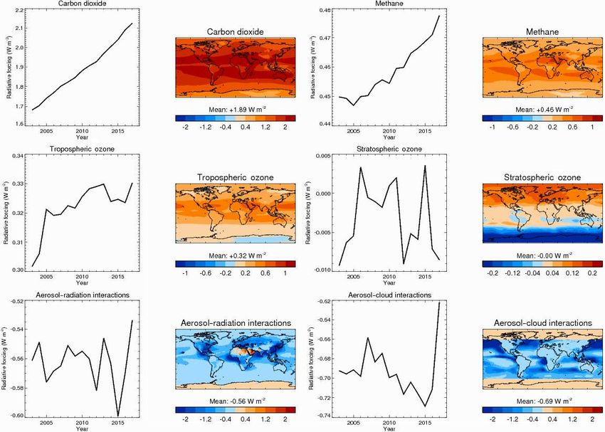
1650                                                                    N. Bellouin et al.: Radiative forcing of climate change

1   Introduction                                                   and longwave radiation, a process called aerosol–radiation
                                                                   interactions (ari; Boucher et al., 2013). Aerosols also exert
                                                                   an RF indirectly through their roles as cloud condensation
Human activities have profoundly modified the composition          nuclei (CCN), which regulate cloud droplet number con-
of the Earth’s atmosphere. They have increased the con-            centration and therefore cloud albedo. Those processes are
centrations of greenhouse gases, with concentrations of car-       called aerosol–cloud interactions (aci; Boucher et al., 2013).
bon dioxide increasing from 278 to 407 ppm (an increase of         Quantifying RF is a difficult task. It strongly depends on the
46 %) and methane from 722 to 1858 ppb (+157 %) over               horizontal and vertical distributions of the forcing agents,
the period 1750–2018 (Dlugokencky et al., 2019). Con-              which in the case of ozone and aerosols are very heteroge-
centrations of aerosols and tropospheric ozone (Hartmann           neous. It depends on the ability of forcing agents to interact
et al., 2013) are frequently above pre-industrial levels in        with radiation, which is difficult to characterise well in the
many regions, especially those that are the most densely           case of chemically diverse species like aerosols (Bellouin
populated. The stratospheric ozone layer is only begin-            et al., 2020a) or may be incompletely represented in many
ning its recovery after being affected by emissions of man-        radiative-transfer codes (e.g. Collins et al., 2006; Etminan
made ozone-depleting substances in the 1970–1980s (WMO,            et al., 2016). RF is defined with respect to an unperturbed
2018). Those modifications have important impacts on hu-           state, typically representing pre-industrial (PI) conditions,
man health and prosperity and on natural ecosystems. One           which is very poorly known for the short-lived forcing agents
of the most adverse effects of human modification of atmo-         like ozone and aerosols (Myhre et al., 2013a; Carslaw et al.,
spheric composition is climate change.                             2013). RF also depends on the ability to understand and cal-
    A perturbation to the Earth’s energy budget leads to tem-      culate the distributions of radiative fluxes with accuracy (So-
perature changes and further climate responses. The initial        den et al., 2018), including the contributions of clouds and
top-of-atmosphere imbalance is the instantaneous radiative         the surface. Those difficulties translate into persistent uncer-
forcing. Several decades ago, it was realised that for compar-     tainties attached to IPCC radiative-forcing estimates. Those
ison of climate change mechanisms the radiative flux change        difficulties are compounded by the lack of consistent and in-
at the tropopause, or equivalently at the top of the atmosphere    tegrated quantifications across forcing agents. In the IPCC
after stratospheric temperatures are adjusted to equilibrium,      Fifth Assessment Report (AR5) (Myhre et al., 2013a), car-
was a better predictor for the surface temperature change and      bon dioxide and methane radiative forcing were derived from
defined as radiative forcing (RF) (Ramanathan, 1975; Shine         fits to line-by-line radiative-transfer models (Myhre et al.,
et al., 1990; Ramaswamy et al., 2019). The adjustment time         1998) using global-mean changes in surface concentrations
in the stratosphere is of the order of 2 to 3 months and is sev-   as input. Aerosol radiative forcing from interactions with
eral orders of magnitude shorter than the time required for        radiation was based on global modelling inter-comparisons
the surface–tropospheric system to equilibrate after a (time-      (Myhre et al., 2013b; Shindell et al., 2013a) and observation-
independent) perturbation. More recently the effective ra-         based estimates (Bond et al., 2013; Bellouin et al., 2013).
diative forcing (ERF) has been defined to include rapid ad-        Aerosol radiative forcing from interactions with clouds was
justments, where, in addition to the stratospheric tempera-        based on many satellite- and model-based studies (Boucher
ture adjustment, these adjustments occur due to heating or         et al., 2013). Ozone radiative forcing was based on results
cooling of the troposphere in the absence of a change in the       from the Atmospheric Chemistry and Climate Model Inter-
ocean surface temperature (Boucher et al., 2013; Myhre et          comparison Project (ACCMIP) (Stevenson et al., 2013; Con-
al., 2013a; Sherwood et al., 2015; Ramaswamy et al., 2019).        ley et al., 2013).
For certain climate change mechanisms, especially those in-            The development of observing and modelling systems able
volving aerosols, the rapid adjustments are important, but in      to monitor and forecast changes in atmospheric composition
many cases, notably the well-mixed greenhouse gases, RF is         offers an attractive way to alleviate some of these difficul-
relatively similar to ERF (Smith et al., 2018a). In principle,     ties. One of those systems is the reanalysis routinely run by
the ERF is a better predictor of surface temperature change        the Copernicus Atmosphere Monitoring Service (CAMS; In-
than RF but is less straightforward to quantify for all forcing    ness et al., 2019), which crowns more than a decade of scien-
mechanisms (see, e.g. Ramaswamy et al., 2019). The quan-           tific endeavours (Hollingsworth et al., 2008) rendered possi-
tification of RF has been a central part of every Assessment       ble by the impressive increase in observing capabilities and
Report of the Intergovernmental Panel on Climate Change            numerical weather prediction over the past 40 years (Bauer et
(IPCC) (Shine et al., 1990; Schimel et al., 1996; Ramaswamy        al., 2015). The CAMS reanalysis combines, in a mathemat-
et al., 2001; Forster et al., 2007; Myhre et al., 2013a).          ically optimal way, many diverse observational data sources
    Carbon dioxide, methane, and ozone exert an RF by ab-          (see Table 2 of Inness et al., 2019) from ground-based and
sorbing and emitting longwave (LW), or terrestrial, radiation      space-borne instruments, with a numerical weather predic-
and absorbing shortwave (SW), or solar, radiation. Aerosols        tion model (see Table 1 of Inness et al., 2019) that also rep-
exert an RF directly by scattering and absorbing shortwave

Earth Syst. Sci. Data, 12, 1649–1677, 2020                                         https://doi.org/10.5194/essd-12-1649-2020
N. Bellouin et al.: Radiative forcing of climate change                                                                      1651

resents the sources and sinks of carbon dioxide and methane
and the complex chemistry governing the concentrations of
ozone and aerosols. Reanalysis products therefore give a
complete and consistent picture of the atmospheric compo-
sition of the past, covering in the case of CAMS the period
2003 to the present. Reanalysis products are therefore a ro-
bust basis for estimating RF of climate change.
   This article describes the RF estimates of carbon diox-
ide, methane, aerosol, and ozone made as part of the CAMS
from its reanalysis of atmospheric composition. The article
starts by describing the methods used to estimate RF from
the reanalysis in Sect. 2, before discussing how the PI ref-
erence state is estimated for the different forcing agents in    Figure 1. Diagram of the radiative-forcing production chain (light
Sect. 3. Section 4 describes the estimates of uncertainties      orange), which takes inputs from the CAMS global reanalysis (blue)
in CAMS RF. Section 5 presents the results over the pe-          and produces radiative-forcing estimates and their uncertainties
riod 2003–2017, discussing distributions and temporal rate       (dark orange). Green boxes indicate observational constraints. BB
of change and comparing these to previous estimates from         stands for biomass burning, and AOD stands for aerosol optical
the IPCC. Section 6 concludes by describing potential uses       depth. ecRad is the radiative-transfer code used by the ECMWF
for the CAMS radiative-forcing products and outline further      IFS.
research avenues that would improve the estimates further.

                                                                 (Morcrette et al., 2009) cycle 42r1. The version of IFS used
2    Methods                                                     has a horizontal resolution of 80 km (T255) and 60 hybrid
                                                                 sigma–pressure levels in the vertical, with the top level at
CAMS estimates follow the definitions for instantaneous and
                                                                 0.1 hPa. The time step is 30 min, with output analyses and
stratospherically adjusted RF given in the IPCC AR5 (Myhre
                                                                 forecasts produced every 3 h. In addition, the reanalysis in-
et al., 2013a).
                                                                 cludes assimilation of satellite retrievals of atmospheric com-
    – Instantaneous RF (IRF) is the “instantaneous change        position, thus improving RF estimates compared to free-
      in net (down minus up) radiative flux (shortwave plus      running models. Improvements derive directly from observa-
      longwave; in W m−2 ) due to an imposed change.”            tional constraints on reactive gas columns and aerosol optical
                                                                 depths (Benedetti et al., 2009) and, for ozone, vertical pro-
    – Stratospherically adjusted RF (hereafter simply referred   files. Data assimilation also constrains gaseous and biomass-
      to as RF) is “the change in net irradiance at the          burning aerosol emissions, leading to indirect improvements
      tropopause after allowing for stratospheric temperatures   in the simulation of atmospheric concentrations. The RF pro-
      to readjust to radiative equilibrium, while holding sur-   duction chain therefore relies primarily on variables tied to
      face and tropospheric temperatures and state variables     observations by the data assimilation process (gas mixing ra-
      such as water vapour and cloud cover fixed at the un-      tios, total aerosol optical depth). However, it is not possible
      perturbed values”.                                         to solely rely on assimilated variables because other charac-
The reference state is taken to be the year 1750. CAMS IRF       teristics of the model affect RF directly (vertical profiles of
and RF are quantified in terms of irradiance changes at the      aerosols and gases, speciation of total aerosol mass) or in-
top of the atmosphere (TOA), the surface, and the climato-       directly (cloud cover and cloud type, surface albedo). Some
logical tropopause for carbon dioxide, methane, and ozone,       other variables relevant for the RF computations (e.g. tem-
although it is noted that RF is necessarily identical at TOA     perature and moisture profiles) are constrained by the assim-
and tropopause. RF is not estimated for tropospheric aerosol     ilation of meteorological parameters, which also indirectly
perturbations because it differs only slightly from IRF at the   affects the cloud structure and transport in the assimilated
TOA (Haywood and Boucher, 2000). CAMS RF estimates               state. In addition, parameters required by the RF estimate but
are quantified in both “all-sky” conditions, meaning that        not simulated by the global reanalysis (e.g. aerosol size dis-
the radiative effects of clouds are included in the radiative-   tributions) are provided by ancillary datasets.
transfer calculations, and “clear-sky” conditions, which are
computed by excluding clouds in the radiative-transfer cal-      2.1   Radiative-transfer calculations
culations.
   Figure 1 illustrates the sequence of tasks that produce the   The radiative-transfer model used is a stand-alone version of
CAMS RF estimates. The source of atmospheric composi-            the ECMWF IFS ecRad model (Hogan and Bozzo, 2018),
tion data is the CAMS reanalysis (Inness et al., 2019) per-      version 0.9.40, configured like in IFS cycle 43r1. Gaseous
formed with the ECMWF Integrated Forecast System (IFS)           optical properties are computed by the Rapid Radiative

https://doi.org/10.5194/essd-12-1649-2020                                        Earth Syst. Sci. Data, 12, 1649–1677, 2020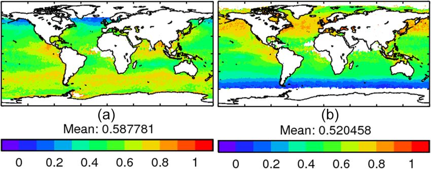
1652                                                                   N. Bellouin et al.: Radiative forcing of climate change

Table 1. Values of LW surface emissivity used for the LW atmo-
spheric window in the radiative-transfer calculations.

               Surface type          LW emissivity
               Land (except sand                0.96
               and snow)
               Sand                             0.93
               Sea                              0.99
               Snow                             0.98

Transfer Model – General Circulation Model (GCM) appli-
cations (RRTMG) (Mlawer et al., 1997). The cloud solver is
the SPeedy Algorithm for Radiative TrAnsfer through CloUd         Figure 2. Time series of globally and monthly averaged concen-
Sides (SPARTACUS) (Hogan et al., 2018). The LW and SW             trations of (a) carbon dioxide (ppm) and (b) methane (ppb) over
                                                                  the period 2003–2017. Bold lines show mass-weighted total column
solvers are based on the Monte Carlo Independent Column
                                                                  averages for the CAMS Greenhouse Flux Inversion products. Thin
Approximation (McICA; Pincus et al., 2003). Surface albedo        lines show background surface measurements from NOAA’s Earth
is calculated by the CAMS reanalysis based on a snow-             System Research Laboratory for carbon dioxide and the Advanced
free surface albedo over land in the UV-visible (0.3–0.7 µm)      Global Atmospheric Gases Experiment for methane, respectively.
and the near-infrared (0.7–5.0 µm) derived from a 5-year cli-
matology by the Moderate Resolution Spectral Radiometer
(MODIS) (Schaaf et al., 2002) and over ocean on a fit of
aircraft measurements (Taylor et al., 1996). The albedo also      decimal place) changes in globally averaged RF. Daily av-
includes the effect of snow cover and sea ice as simulated by     eraged concentrations of carbon dioxide and methane are
the CAMS reanalysis. LW surface emissivity is computed by         taken from the data-assimilated, three-dimensional distribu-
averaging the spectrally constant emissivity of four surface      tions obtained by CAMS Greenhouse Gases Fluxes (Cheval-
tiles in proportion to their simulated coverage of each grid      lier et al., 2005; Bergamashi et al., 2013) for carbon diox-
box. Surface window emissivities used in that calculation are     ide and methane, respectively, with updates to both doc-
listed in Table 1. Outside the LW window region, the value        umented at https://atmosphere.copernicus.eu (last access:
for sea is used. Cloud vertical overlap is assumed to be expo-    14 July 2020). Nitrous oxide is set to its pre-industrial
nential random. Scattering by clouds and aerosols in the LW       mixing ratio of 270 ppb (Myhre et al., 2013a). The in-
spectrum is included. RF is integrated diurnally over six so-     version product versions used are v18r2 for carbon diox-
lar zenith angles, computed as a function of local latitude and   ide and v17r1 for methane. Figure 2 shows time series
day of the year, and symmetrically distributed around local       of global monthly total-column averages of carbon dioxide
noon. Radiative fluxes are calculated at 61 model half-levels,    and methane concentrations. The annually averaged carbon
but for RF purposes only three levels are retained: surface,      dioxide concentration in 2017 was 404 ppm, up 8 % from
TOA, and tropopause. The tropopause level is identified daily     374 ppm in 2003. For methane, the concentration for year
according to its thermal definition, adopted by the World Me-     2017 was 1804 ppb, up 4 % from 1730 ppb in 2003. Figure 2
teorological Organization (WMO), where the tropopause is          also shows equivalent time series for background surface
the lowest altitude at which lapse rate drops to 2 K km−1 . In    measurements by the NOAA Earth System Research Lab-
its standard version, ecRad uses fixed values for the effec-      oratory (downloaded from https://www.esrl.noaa.gov/gmd/
tive radius of cloud liquid droplets and ice crystals at 10 and   ccgg/trends/global.html#global_data, last access: 14 July
50 µm, respectively. The calculations of radiative fluxes by      2020) for carbon dioxide and by the Advanced Global Atmo-
the radiative-transfer code have been compared against glob-      spheric Gases Experiment (AGAGE, downloaded from https:
ally averaged observational estimates (Kato et al., 2013) and     //agage.mit.edu/data/agage-data, last access: 14 July 2020)
found to be accurate within a few percent.                        for methane. Surface measurements are generally higher than
   The distributions taken from the CAMS reanalysis as in-        the column averages, especially for methane that decreases
puts to the CAMS radiative-transfer calculations are listed in    with height by oxidation.
Table 2. The distributions are used as the mean of four time         Adjustment of radiative fluxes to account for changes in
steps (00:00, 06:00, 12:00, and 18:00 Z) for the reanalysis       stratospheric temperatures uses the fixed dynamical heating
dated 00:00 Z daily. The distributions are used at the de-        (FDH) method (Ramaswamy et al., 2001). Convergence is
graded horizontal resolution of 3.0◦ × 3.0◦ , down from the       reached when globally averaged changes in heating rate, RF,
original 0.75◦ × 0.75◦ resolution, to reduce computational        and stratospheric temperature become less than 0.05 K d−1 ,
cost. That decrease in resolution causes negligible (third        0.05 W m−2 , and 0.01 K, respectively. The maximum num-

Earth Syst. Sci. Data, 12, 1649–1677, 2020                                        https://doi.org/10.5194/essd-12-1649-2020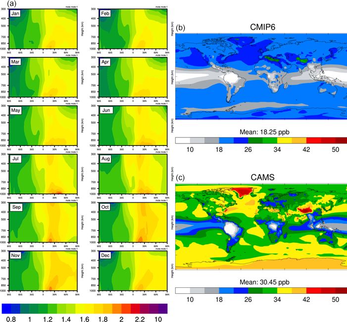
N. Bellouin et al.: Radiative forcing of climate change                                                                                  1653

Table 2. List of variables used by the offline radiative-transfer model ecRad and their provenance. All variables are set as daily averages.

              Variable                                        Provenance
              Atmospheric and surface state
              Fraction of cloud cover                         CAMS reanalysis
              Forecast albedo (surface)                       CAMS reanalysis (includes the effect of snow and sea ice cover)
              Logarithm of surface pressure                   CAMS reanalysis
              Specific cloud ice water content                CAMS reanalysis
              Specific cloud liquid water content             CAMS reanalysis
              Skin temperature                                CAMS reanalysis
              Snow depth                                      CAMS reanalysis
              Soil type                                       CAMS reanalysis
              Specific humidity                               CAMS reanalysis
              Temperature                                     CAMS reanalysis
              Atmospheric composition
              Sea salt (0.03–0.5, 0.50–5.0, 5.0–20.0 µm)      CAMS reanalysis
              Dust (0.03–0.55, 0.55–0.90, 0.90–20.0 µm)       CAMS reanalysis
              Hydrophilic organic matter                      CAMS reanalysis
              Hydrophobic organic matter                      CAMS reanalysis
              Hydrophilic black carbon                        CAMS reanalysis
              Hydrophobic black carbon                        CAMS reanalysis
              Ammonium sulfate                                CAMS reanalysis
              Non-abs stratospheric sulfate                   CAMS reanalysis
              GEMS ozone                                      CAMS reanalysis
              CH4 mixing ratio                                Atmospheric concentrations from CAMS73
              CO2 mixing ratio                                Atmospheric concentrations from CAMS73
              Industrial-era increments
              Pre-industrial CH4 mixing ratio                 Scaled to match IPCC AR5 Table 8.2; see Sect. 3.1
              Pre-industrial CO2 mixing ratio                 Scaled to match IPCC AR5 Table 8.2; see Sect. 3.1
              Pre-industrial O3 mixing ratio                  Scaled according to CMIP6 ozone climatology; see Sect. 3.2

ber of iterations is also set to 200. Once stratospheric adjust-             – Aerosol origin is not always given in emission invento-
ment is complete, the sum of the SW + LW radiative fluxes                      ries.
at the tropopause equals that at the top of the atmosphere.
Methane RF is given in the LW and SW parts of the spec-                      – The same aerosol particle may be an internal mixture
trum, although it is now known that ecRad – similar to many                    with anthropogenic and natural contributions.
other radiative-transfer codes used in global models – is un-                – Data assimilation cannot constrain natural and anthro-
likely to properly handle methane absorption bands in the                      pogenic aerosols separately.
SW part of the spectrum because it does not have sufficient
spectral resolution. Therefore, the CAMS products likely un-               Instead, aerosol origin is obtained using the algorithm de-
derestimate methane RF in the SW spectrum, and that under-                 scribed by Bellouin et al. (2013), where aerosol size is used
estimate affects its stratospheric adjustment. The SW con-                 as a proxy for aerosol origin. The algorithm identifies four
tribution may be of the order of 15 % of total methane RF                  aerosol origins: anthropogenic, mineral dust, marine, and
(Etminan et al., 2016).                                                    land-based fine-mode natural aerosol. The latter originates
                                                                           mostly from biogenic aerosols. The reader is referred to
2.2   Aerosol–radiation interactions                                       Sect. 3 of Bellouin et al. (2013) for details of the algorithm.
                                                                           The present paper describes two updates made to the algo-
To obtain aerosol RF, it is necessary to distinguish between               rithm since the publication of Bellouin et al. (2013).
aerosols of natural origin and aerosols of anthropogenic ori-                 The first update is the replacement of continental-wide
gin. The ECMWF IFS does not keep track of the aerosol ori-                 anthropogenic fractions used over land surfaces by a fully
gin mainly to keep computational cost reasonable but also                  gridded dataset that includes seasonal variations. Over land,
due to the following reasons.                                              identification of component aerosol optical depths (AODs)
                                                                           starts with removing the contribution of mineral dust aerosols

https://doi.org/10.5194/essd-12-1649-2020                                                  Earth Syst. Sci. Data, 12, 1649–1677, 2020
1654                                                                  N. Bellouin et al.: Radiative forcing of climate change

                                                                 Figure 4. Fine-mode fraction of marine aerosol optical depth at
                                                                 0.55 µm as derived from MODIS/Terra Collection 6 aerosol re-
                                                                 trievals for the months of January (a) and July (b).

Figure 3. Annually averaged anthropogenic fraction of non-dust
aerosol optical depth over land at 0.55 µm.
                                                                 at 0.55 µm is between 0.03 and 0.10. Then, an AOD-weighted
                                                                 averaged FMF is computed. The analysis has been applied
from total AOD. The remaining non-dust AOD, τnon-dust , is
                                                                 to retrievals from MODIS instruments on both the Terra
then distributed between anthropogenic and fine-mode nat-
                                                                 (dataset covering 2001–2015) and Aqua (dataset covering
ural components, referred to as τanth and τfine-mode , respec-
                                                                 2003–2015) platforms. Both instruments yield very similar
tively, as follows:
                                                                 marine FMF distributions, and the distributions used here are
τanth = fanth · τnon-dust ,                                (1)   the multi-annual monthly averages of the two instruments.
τfine-natural = (1 − fanth ) · τnon-dust ,                 (2)   Figure 4 shows the marine FMF derived from MODIS/Terra
                                                                 for the months of January and July. It suggests that marine
where fanth is the anthropogenic fraction of the non-dust        FMF varies over a wide range of values. Regions of high
AOD. In Bellouin et al. (2013), fanth was prescribed over        wind speeds, around 40–50◦ in both hemispheres, are asso-
broad regions on an annual basis. Here, fanth is given by        ciated with large FMFs, indicating that the marine aerosol
monthly distributions on a 1◦ × 1◦ grid. This new dataset        size distribution includes a sizable fraction of smaller par-
derives from an analysis of AeroCom 2 numerical mod-             ticles there. There are indications of contamination by fine-
els (Kinne et al., 2013). Its annual average is shown in         mode anthropogenic and mineral dust aerosols in coastal ar-
Fig. 3. Anthropogenic fractions show a north–south gradi-        eas, but the impact on speciated AODs is small because the
ent, as expected from the location of population and in-         aerosol identification algorithm uses broad FMF categories
dustrial activities. Anthropogenic fractions are larger than     rather than absolute values. Indeed, anthropogenic AOD de-
0.8 over most industrialised regions of North America, Eu-       creases only slightly in the roaring forties in the Southern
rope, and Asia. The largest fractions are located over China,    Ocean and tends to increase slightly in the northern Atlantic
where more than 90 % of non-dust AOD is attributed to an-        and Pacific oceans. On a global average, the change in an-
thropogenic aerosols. In the Southern Hemisphere, anthro-        thropogenic AOD due to the improved specification of ma-
pogenic fractions are typically smaller than 0.7 on an an-       rine FMF is +0.001 (+1.4 %). Bellouin et al. (2013) esti-
nual average. In terms of seasonality, anthropogenic fractions   mated the relative uncertainty in τanth at 18 %. The updates
remain larger than 0.7 throughout the year in the Northern       to land-based anthropogenic fractions and marine FMF de-
Hemisphere, with a peak in winter when energy consumption        scribed here are not expected to reduce their large contribu-
is high. In the Southern Hemisphere, seasonality is driven by    tion to that uncertainty.
biomass-burning aerosols, which are considered purely an-           Radiative effect and forcing of aerosol–radiation inter-
thropogenic in the CAMS Climate Forcing estimates. An-           actions are computed by radiative-transfer calculations that
thropogenic fractions therefore peak in late boreal summer       combine the speciated AODs derived above with prescrip-
in South America and southern Africa.                            tions of aerosol size distribution and single-scattering albedo.
   The second change concerns the fine-mode fraction (FMF)       The methods are as described in Sect. 4 of Bellouin et
of marine AOD at 0.55 µm, which gives the fraction of            al. (2013) with one exception: the prescription of single-
marine AOD that is exerted by marine particles with radii        scattering albedo has been updated from a few continental-
smaller than 0.5 µm. In Bellouin et al. (2013), this fraction    wide numbers to gridded monthly climatologies. This up-
was set to a fixed value of 0.3. Here, this fraction is deter-   dated dataset introduces two major improvements compared
mined by a gridded dataset that includes monthly variations.     to Bellouin et al. (2013). First, the new dataset provides the
The dataset is obtained by applying the method of Yu et          monthly cycle of fine-mode absorption. Second, the dataset is
al. (2009) to daily MODIS Collection 6 aerosol retrievals of     provided on a finer, 1◦ ×1◦ grid. The method used to produce
AOD and FMF. First, the marine aerosol background is iso-        the dataset is described in Kinne et al. (2013). First, distribu-
lated by selecting only ocean-based scenes where total AOD       tions of fine-mode extinction and absorption AODs are ob-

Earth Syst. Sci. Data, 12, 1649–1677, 2020                                       https://doi.org/10.5194/essd-12-1649-2020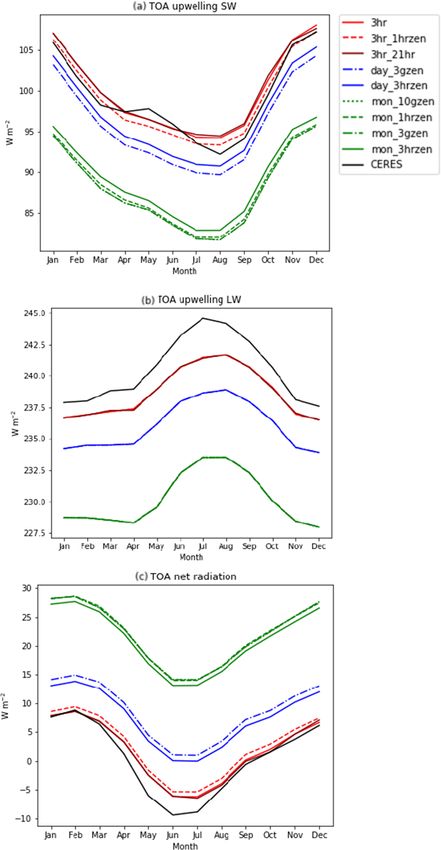
N. Bellouin et al.: Radiative forcing of climate change                                                                          1655

                                                                      cloud anthropogenic and mineral dust AODs weighted by
                                                                      cloud fraction are 0.005 and 0.003, respectively, or 8 % of
                                                                      their clear-sky counterparts. Above-cloud marine and fine-
                                                                      mode natural AODs are negligible. Above-cloud anthro-
                                                                      pogenic aerosols exert a positive radiative effect because of
                                                                      their absorbing nature and the high reflectance of clouds.
                                                                      Those radiative effects commonly reach +5 to +10 W m−2
                                                                      locally during the biomass-burning season that lasts from
                                                                      late August to October over the south-eastern Atlantic stra-
                                                                      tocumulus deck. However, this only translates into a cloudy-
                                                                      sky anthropogenic RFari of +0.01 W m−2 , in agreement with
                                                                      AeroCom-based estimates, which span the range +0.01 ±
Figure 5. Annually averaged distribution of column-averaged           0.1 W m−2 (Myhre et al., 2019). Studies based on the Cloud-
single-scattering albedo at 0.55 µm used to characterise absorption   Aerosol Lidar with Orthogonal Polarization (CALIOP) esti-
of anthropogenic aerosols.                                            mate that all-sky radiative effects of present-day above-cloud
                                                                      aerosols range between 0.1 and 0.7 W m−2 on an annual av-
                                                                      erage over 60◦ S to 60◦ N (Oikawa et al., 2018; Kacene-
tained from a selection of global aerosol numerical models            lenbogen et al., 2019), but only a fraction of that radiative
that participated in the AeroCom simulations using a com-             effect contributes to RFari because of compensations from
mon set of aerosol and precursor emissions for present-day            pre-industrial biomass-burning aerosols. Neglecting above-
conditions (Kinne et al., 2006). To include an observational          cloud aerosols therefore introduces a small uncertainty into
constraint, those modelled distributions are then merged with         the global average but leads to larger errors regionally and
retrievals of aerosol single-scattering albedo (SSA) for the          seasonally.
period 1996–2011 at more than 300 AERONET sites. The
merging is based on a subjective assessment of the quality            2.3    Aerosol–cloud interactions
of the measurements at each of the AERONET sites used,
along with their ability to represent aerosols in a wider re-         The algorithm that estimates the RF of aerosol–cloud in-
gion around the site location. The main impact of merg-               teractions (RFaci) is the same as that used in Bellouin et
ing observed SSAs is to make aerosols in Africa and South             al. (2013). It is based on satellite-derived cloud susceptibil-
Asia more absorbing than numerical models predicted. The              ities to aerosol changes, which are given seasonally and re-
distribution of annual and column-averaged aerosol SSA is             gionally. Statistics of satellite retrievals of liquid clouds are
shown in Fig. 5. The dataset represents the local maximum             poor at high latitudes (Grosvenor et al., 2018), so cloud sus-
of absorption over California and the change in absorption as         ceptibilities are not available poleward of 60◦ and RFaci is
biomass-burning aerosols age during transport, which is vis-          not estimated there. Aerosol changes are obtained by the an-
ible over the south-eastern Atlantic. Over Asia, Europe, and          thropogenic AOD derived in Sect. 2.2. The cloud susceptibil-
South America, absorption is also larger near source regions,         ities are applied to low-level (warm) clouds only.
with less absorption elsewhere.
   It is worth noting that the SSA distribution characterises         3     Pre-industrial state
absorption of fine-mode aerosols but is used to provide the
absorption of anthropogenic aerosols, which is not fully con-         3.1    Carbon dioxide and methane
sistent. The inconsistency is, however, mitigated by two fac-
                                                                      The three-dimensional distributions of carbon dioxide and
tors. First, fine-mode aerosols are the main proxy for anthro-
                                                                      methane derived for present-day (PD) strongly benefit from
pogenic aerosols in the Bellouin et al. (2013) algorithm that
                                                                      data assimilation of surface measurements and satellite re-
identifies aerosol origin, and their distributions are broadly
                                                                      trievals, which partly offset the biases of the chemistry
similar. Second, regions where natural aerosols such as ma-
                                                                      model. That, however, creates the difficulty that estimating PI
rine and mineral dust may contaminate the fine-mode AOD
                                                                      concentrations by running the chemistry model with PI emis-
often correspond to minima in anthropogenic AOD.
                                                                      sions would be biased with respect to the data-assimilated,
   Like in Bellouin et al. (2013), the RF of aerosol–radiation
                                                                      present-day distributions. Instead, daily PI mixing ratios of
interactions (RFari) is estimated in clear-sky (cloud-free sky)
                                                                      carbon dioxide and methane are scaled from daily CAMS
then scaled by the complement of the cloud fraction in each
                                                                      Greenhouse Gas Flux mixing ratios in each grid box and at
grid box to represent all-sky conditions, thus assuming that
                                                                      each model level using the following equation:
cloudy-sky aerosol–radiation interactions are zero. Experi-
mental estimates of cloudy-sky RF have been done but are
based on a simplified account of cloud albedo, which limits
their usefulness. For the year 2003, globally averaged above-

https://doi.org/10.5194/essd-12-1649-2020                                             Earth Syst. Sci. Data, 12, 1649–1677, 2020
1656                                                                       N. Bellouin et al.: Radiative forcing of climate change

                                                                     stratosphere, allowing for mutual influence. Historical strato-
                  D              E                                   spheric ozone reflects the effects of long-lived greenhouse
                   [X]AR5
                      PI,surface                                     gases such as carbon dioxide, nitrous oxide, and methane in
[X]PI = [X]PD ·                      ,                        (3)    a physically and chemically consistent way. The interannual
                  [X]PD,surface
                                                                     variability, including the Quasi-Biennial Oscillation, is in-
where [X] denotes the mixing ratio of carbon dioxide or              cluded. The CMAM pre-industrial control configuration uses
methane, and angle brackets denote annual averaging. All             precursor and greenhouse gas emissions for the year 1850 in
variables are taken from the CAMS GreenhouseD Gas Flux in-      E    a 40-year simulation, with the last 10 years used to create the
versions, except for PI surface mixing ratios, [X]AR5                mean ozone field. The WACCM pre-industrial control con-
                                                      PI,surface ,
which come from footnote a of Table 8.2 of Myhre et                  figuration averages precursor and greenhouse gas emissions
al. (2013a), 278 ppm for carbon dioxide and 772 ppb for              over the 1850–1859 period. The reference spectral and total
methane. The scaling factors are calculated at the surface be-       irradiances are derived from averages over the period 1834–
cause this is the level where PI concentrations are given in         1867 (solar cycles 8–10), but the 11-year solar cycle is not
Myhre et al. (2013a): the whole profile is scaled like the sur-      considered.
face level, which is justified by the relatively well-mixed na-         Figure 6 shows the monthly cross sections of the PD-to-
ture of both gases. By construction, the scaled PI distribution      PI ratios used to scale CAMS reanalysis ozone mixing ra-
has the same global, annual average value at the surface as          tios following the equation above. The ratios exhibit a strong
given in Myhre et al. (2013a) but inherits the horizontal, ver-      hemispheric contrast. In the Northern Hemisphere, ratios are
tical, and temporal variabilities of the PD distribution. Using      typically larger than 1.5 throughout the year and can be
this scaling method replicates the PD amplitude of the sea-          around 2 in the lower troposphere above polluted regions. In
sonal cycle of carbon dioxide and methane concentrations.            the Southern Hemisphere, ratios are closer to 1.2 and are be-
For carbon dioxide, there is a suggestion from modelling             low 1 in the upper tropospheric Antarctic ozone hole, where
studies that the amplitude of the seasonal cycle may have            the ozone layer has been diminished since PI conditions. Fig-
increased since PI (Lindsay et al., 2014). Replicating the PD        ure 6 also compares surface ozone volume mixing ratios in
amplitude would therefore cause a small underestimate of the         the Hegglin et al. (2016) dataset for the year 1850 to those
forcing.                                                             resulting from scaling CAMS reanalysis ozone concentra-
                                                                     tions, averaged over the period 2003–2016. CAMS PI sur-
                                                                     face ozone is about 1.7 larger than in the Hegglin et al. (2016)
3.2    Ozone                                                         dataset. The global distribution of PI ozone concentrations is
Like carbon dioxide and methane, ozone distributions in the          poorly known due to a lack of measurements in different re-
CAMS reanalysis are strongly affected by data assimilation           gions of the world, but ACCMIP models (Young et al., 2013)
of ozone profiles and total and partial columns (Inness et al.,      and the isotopic analysis of Yeung et al. (2019) suggest that
2015). Consequently, it is also not advisable to simply simu-        the PI ozone levels in the Northern Hemisphere were of the
late PI ozone concentrations by running the chemistry model          order of 20 to 30 ppbv in the Northern Hemisphere and 10
with PI emissions, as that would introduce biases between a          to 25 ppbv in the Southern Hemisphere. CAMS estimates are
data-assimilated PD and a free-running PI. Instead, daily PI         higher, probably because of overestimations of surface ozone
ozone mixing ratios are scaled in each grid box and at each          in the CAMS reanalysis, especially in the Tropics and North-
model level from daily CAMS reanalysis mixing ratios as              ern Hemisphere (Inness et al., 2019), which propagate to the
follows:                                                             PI estimates. Although it will be good to reduce those bi-
                                                                     ases in future versions of the dataset, the fact that both PI
                      [O3 ]CMIP6
                           PI                                        and PD ozone concentrations are similarly biased should not
[O3 ]PI = [O3 ]PD ·                  ,                        (4)
                      [O3 ]CMIP6                                     have a large impact on tropospheric ozone RF, which mostly
                           PD
                                                                     depends on the PI to PD increment in ozone concentrations.
where [O3 ] denotes ozone mixing ratios and angle brackets
denote monthly averaging. [O3 ]CMIP6
                                  PD    and [O3 ]CMIP6
                                                 PI     are          3.3   Aerosols
taken from the three-dimensional CMIP6 input4MIPs ozone
concentration dataset of Hegglin et al. (2016), briefly de-          The anthropogenic AOD (Sect. 2.2), which is then used to
scribed by Checa-Garcia et al. (2018), for the years 2008–           estimate RFari and RFaci, is defined with respect to PD nat-
2012 for PD and 1850–1899 for PI. The Hegglin et al. (2016)          ural aerosols, which is a different reference to PI (1750) so a
dataset was obtained by merging 10-year running-averaged             correction is required (Bellouin et al., 2008). That correction
simulated ozone distributions by the Canadian Middle Atmo-           factor is taken from Bellouin et al. (2013) and is equal to 0.8;
sphere Model (CMAM) and the Whole Atmosphere Chem-                   i.e. RFari and RFaci defined with respect to PI are 80 % of
istry Climate Model (WACCM), both driven by CMIP5 his-               RFari and RFaci defined with respect to PD natural aerosols.
torical emissions (Lamarque et al., 2010). The models re-
solve the chemistry and dynamics of the troposphere and

Earth Syst. Sci. Data, 12, 1649–1677, 2020                                            https://doi.org/10.5194/essd-12-1649-2020
N. Bellouin et al.: Radiative forcing of climate change                                                                           1657

Figure 6. (a) Monthly averaged zonal cross sections of ratios of present-day (2008–2014) to pre-industrial (1850–1900) ozone mass-mixing
ratios from the CMIP6 input4MIPs climatology. Surface ozone volume mixing ratios (in ppb) in (b) the CMIP6 input4MIPs climatology and
(c) scaled from the CAMS reanalysis using the ratios shown on the left.

4   Uncertainties                                                     transfer equation is solved) in addition to parametric uncer-
                                                                      tainty. Parametric uncertainty is also present from the choices
                                                                      of which refractive index to use for calculating aerosol scat-
Model uncertainty can be structural or parametric in nature.          tering and absorption processes.
The structural uncertainty relates to methodological and pa-
rameterisation choices in the characterisation of the radia-
                                                                      4.1   Uncertainty from methodological choices
tive forcing. It is known to be influenced by the atmospheric
time step used in evaluating the radiative forcing (Colman et         All experiments in this section are performed using the
al., 2001), the effect of any climatological averaging (Mül-          CAMS reanalysis dataset for the year 2003. Greenhouse gas
menstädt et al., 2019) and for IRF or RF, the definition of           concentrations for carbon dioxide, methane, and nitrous ox-
tropopause (Collins et al., 2006). Parametric uncertainty re-         ide but also for CFC-11, CFC-12, HCFC-22, and CCl4 from
lates to choices of the value of the parameters within the            2003 and 1850 are taken from the Representative Concentra-
parameterisations. As radiation calls are expensive, in cli-          tion Pathways (RCP) historical dataset (Meinshausen et al.,
mate reanalysis or general circulation models the SW and              2011). Although these forcings do not comprise the totality
LW parts of the spectrum are divided into a small number of           of anthropogenic greenhouse gas RF, 98 % of the well-mixed
bands that exhibit similar scattering and absorption proper-          greenhouse gas RF is included from these species according
ties. This parameterisation error can be significant (Collins         to Table 8.2 of Myhre et al. (2013a), which is for the year
et al., 2006; Pincus et al., 2015). Different radiative-transfer      2011.
solvers divide the bands in different ways, and the choice
of radiative-transfer code contributes structural uncertainty
(as there are methodological differences in how the radiative-

https://doi.org/10.5194/essd-12-1649-2020                                             Earth Syst. Sci. Data, 12, 1649–1677, 2020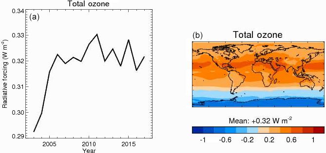
1658                                                                    N. Bellouin et al.: Radiative forcing of climate change

4.1.1   Time stepping and averaging                                ter than monthly. Agreement with observations is less good
                                                                   with the 3-hourly instantaneous radiative fluxes in the LW
Uncertainty relating to time stepping comes from both the          than in the SW. Figure 7c shows net TOA radiation. Again,
resolution of the climatology (the effect of averaging or          3 h instantaneous climatologies agree better with observa-
sampling frequency of the input data), as well as the fre-         tions than daily means, which are in turn better than monthly
quency of the radiation calls. Table 3 summarises the nine         means. Biases with mean climatologies add rather than can-
time-stepping and climatological-averaging experiments un-         cel, as upwelling radiation is underestimated in both the LW
dertaken to quantify that uncertainty. In the IFS, full ra-        and the SW for daily and monthly means. Note that Fig. 7
diation calls are only made every 3 simulated hours, with          and Table 4 suggest that the effect of climatological averag-
reduced radiation calls made on intermediate model time            ing dominates over the frequency of SW radiation calls.
steps (30 min), to mitigate against the high cost of radiative-
transfer calculations. Alongside using 3 h instantaneous data,
reanalysis data are prepared as both daily and monthly means       Radiative forcing at top-of-atmosphere and tropopause
with a range of reduced-frequency radiation call methodolo-        Here, IRF is estimated by comparing all-sky net fluxes at the
gies. In the SW this requires an appropriate choice of solar       tropopause and at the TOA for 2003 and 1850. A simplified
zenith angle. Alongside the standard case of 6 representative      definition of the tropopause is employed for this comparison,
solar zenith angles per day, we investigate 6 and 20 represen-     defined as the 29th model level in the CAMS reanalysis, the
tative zenith angles for monthly averaged climatologies. The       level closest to 200 hPa. Alternative tropopause assumptions
impact of averaged climatologies is also isolated by using 3 h     are investigated below. For the purpose of these experiments,
solar zenith angles with daily and monthly climatologies. In       the 1850 atmosphere is created by adjusting the concentra-
addition, an experiment using instantaneous 3-hourly reanal-       tions of the eight greenhouse gases included in the ecRad
ysis in which we retain every seventh model output time step       code to 1850 levels following Meinshausen et al. (2011).
(i.e. interval of 21 h) is performed. This experiment does not     Mixing ratios of ozone and aerosol species are prescribed
introduce bias from averaging the underlying reanalysis data       using a gridded PI to PD ratio. Meteorology (temperature,
while reducing the number of radiation calls. A 21 h sam-          water vapour, and cloud variables) is fixed at 2003 levels in
pling frequency is chosen to preserve the diurnal and sea-         all experiments.
sonal insolation cycles, as recommended in partial radiative          Figure 8 shows the results for the 3hr, day_3hrzen and
perturbation studies (Colman et al., 2001). The approxima-         mon_3hrzen experiments. In the absence of PI observations,
tions introduced by using a 3-hourly effective zenith angle        the RF calculated in the 3hr experiment is assumed to be
are compared by using the same underlying reanalysis data          closest to the truth, given the better agreement to CERES
with a 1-hourly effective zenith angle. At periods of 1 h or       TOA fluxes than the daily or monthly averaged reanalysis
less, the effective and instantaneous zenith angles are very       data. Corresponding time-stepping experiments for differ-
similar in most grid points.                                       ent solar zenith time steps give almost identical results. SW
                                                                   IRF is deficient when using averaged climatology, with TOA
Top-of-atmosphere flux imbalance                                   mon_3hrzen disagreeing in sign with 3hr. The errors intro-
                                                                   duced in the LW by climatological averaging are relatively
Although the focus of this work is the accuracy of the RF, it      small, amounting to about 6 % at the tropopause and 10 %
is useful to explore the dependency of the present-day sim-        at the TOA for mon_3hrzen compared to 3hr. Although LW
ulation of TOA irradiances on the time-stepping. Figure 7          forcing dominates, the errors in the SW forcing are of larger
shows the results from the time-stepping experiment, and           magnitude, so the net climatological averaging effect is 15 %
root-mean-squared errors (RMSEs) for the simulated data            at the tropopause and 21 % at the TOA. The error in net
versus observations from the Clouds and the Earth’s Radiant        IRF is 0.21 W m−2 at the tropopause for day_3hrzen (and
Energy System, Energy Balanced and Filled dataset (CERES           day_3gzen, not shown) compared to 3hr. This is used as our
EBAF TOA Ed4.0) (Loeb et al., 2018) are given in Table 4.          uncertainty range in the CAMS reanalysis RF product, which
The CERES data assumes a nominal TOA height of 20 km,              is calculated using a day_3gzen methodology.
which is well above the cloud layer, so radiative fluxes are not
significantly different to those at the top level of the model.    4.1.2   Spatial resolution of reanalysis data
Figure 7a shows that accuracy in the SW upwelling TOA ra-
diation is compromised by using climatological averaging.          To determine whether the 3◦ × 3◦ grid resolution for RF cal-
Monthly averaging is 3 to 4 times less accurate than daily av-     culation introduces additional error, the 2003 TOA fluxes
eraging, whereas 3-hourly instantaneous climatologies agree        were analysed using the 3hr_21hr methodology at the native
well with observations. This result agrees with Mülmentstädt       model resolution of 0.75◦ ×0.75◦ . Only minor differences are
et al. (2019). Figure 7b shows the corresponding fluxes for        found in the TOA radiative fluxes: −0.02 W m−2 in the SW
LW outgoing radiation. Again, 3-hourly instantaneous clima-        and +0.07 W m−2 in the LW, resulting in a +0.05 W m−2 net
tologies perform better than daily, which in turn perform bet-     difference. As the pre-industrial ratios of ozone and aerosol

Earth Syst. Sci. Data, 12, 1649–1677, 2020                                        https://doi.org/10.5194/essd-12-1649-2020
N. Bellouin et al.: Radiative forcing of climate change 1659 Figure 7. Radiative fluxes calculated by ecRad using 2003 CAMS reanalysis data for the nine time-stepping experiments described in Table 3 (coloured lines): (a) top-of-atmosphere shortwave upwelling radiative flux, (b) top-of-atmosphere longwave upwelling radiative flux, (c) top-of-atmosphere net downwelling radiation. The black line shows the observed radiation fluxes for CERES EBAF. https://doi.org/10.5194/essd-12-1649-2020 Earth Syst. Sci. Data, 12, 1649–1677, 2020
1660                                                                            N. Bellouin et al.: Radiative forcing of climate change

Table 3. Time-stepping and climatological-averaging experiments.

                    Label            Reanalysis data              Solar zenith angle            Radiation calls per year
                                                                                                 SW      LW       Total
                    3hr              3-hourly instantaneous       3 h effective                 2920    2920      5840
                    3hr_1hrzen       3-hourly instantaneous       1 h effective                 8760    2920     11 680
                    3hr_21hr         3-hourly instantaneous,      3 h effective, every           418     418        836
                                     every 7th model time step    7th model time step
                    day_3hrzen       daily mean                   3 h effective                 2920     365      3285
                    day_3gzen        daily mean                   3 representative Gaussian     1095     365      1460
                    mon_1hrzen       monthly mean                 1 h effective                 8760      12      8772
                    mon_3hrzen       monthly mean                 3 h effective                 2920      12      2932
                    mon_10gzen       monthly mean                 10 representative Gaussian     120      12       132
                    mon_3gzen        monthly mean                 3 representative Gaussian       36      12        48

Figure 8. Global-mean instantaneous radiative forcing for the year 2003 (in W m−2 ) at the tropopause and top of atmosphere for 3-hourly
solar zenith angle time steps for 3-hourly, daily, and monthly climatologies.

precursors are not available on this higher-resolution grid,              tify the impact of that definition on estimated RF (Forster and
IRF cannot be calculated using the finer grid, but IRF errors             Shine, 1997). The uncertainty analysis is done on tropopause
are likely to be even smaller because taking the difference in            IRF because of the large number of radiation calls needed
TOA (or tropopause) fluxes is expected to result in smaller               to produce an FDH estimate of RF. Experiment 3hr_21hr is
errors than the absolute TOA difference. The spatial resolu-              used as a basis to investigate the uncertainty in the tropopause
tion error is assessed to be 0.05 W m−2 .                                 definition for IRF.
                                                                             The default definition of the tropopause used in CAMS
4.1.3   Tropopause definition                                             RF estimates is the WMO definition of the lowest altitude at
                                                                          which lapse rate drops to 2 K km−1 , providing the lapse rate
Figure 8 shows that TOA IRF differs significantly from                    in the 2 km above this level does not exceed 2 K km−1 . The
tropopause IRF – in fact the difference, which is mostly due              tropopause level is calculated daily. Alternative definitions
to carbon dioxide, explains the need for stratospheric tem-               used here are as follows:
perature adjustment. But regardless of whether IRF or RF is
estimated, there is a need to define the tropopause and quan-

Earth Syst. Sci. Data, 12, 1649–1677, 2020                                                https://doi.org/10.5194/essd-12-1649-2020
N. Bellouin et al.: Radiative forcing of climate change 1661
Table 4. Root-mean-square error (RMSE, in W m−2 ) of monthly Table 5. Shortwave, longwave, and net instantaneous radiative forc-
top-of-atmosphere (TOA) radiation compared to CERES-EBAF for ings (in W m−2 ) calculated with different tropopause definitions.
2003.
Definition SW LW Net
Experiment SW TOA LW TOA Net TOA
Level 29 −0.55 2.88 2.33
RMSE RMSE RMSE
200 hPa −0.56 2.88 2.31
3hr 1.07 1.9 1.79 Hansen, 1997 −0.46 2.98 2.52
3hr_1hrzen 1.02 1.9 2.48 Soden, 2008 −0.52 2.92 2.40
3hr_21hr 1.18 1.91 1.74 WMO −0.44 3.01 2.57
day_3gzen 3.78 4.52 8.23 CAMS −0.50 2.97 2.46
day_3hrzen 2.77 4.52 7.18
mon_10gzen 11.25 10.33 21.55
mon_1hrzen 11.26 10.33 21.57
mon_3gzen 11.24 10.33 21.54
as radiative-transfer codes with higher spectral resolution
mon_3hrzen 10.34 10.33 20.65
are too computationally expensive. Structural uncertainty
also arises from the choices of approximations and numer-
ical methods used in the actual solving of the radiative-
– the 200 hPa level, calculated by interpolating ecRad- transfer equation. Parameterisation uncertainty arises from
calculated fluxes on model levels in logarithm of pres- the treatment of scattering and absorption of gases, clouds,
sure, this level is used as a proxy for the tropopause from and aerosols. Further uncertainty is introduced by use of
model results in the RF inter-comparison of Collins et a two-stream radiative-transfer model, which is standard in
al. (2006); most GCMs, as well as in ecRad, again for reasons of effi-
ciency. This component of uncertainty is not quantified here,
– level 29 of the CAMS reanalysis grid, which is closest
but, in the case of RFari, Randles et al. (2013) found bi-
to 200 hPa at most locations and easy to obtain;
ases of both signs due to two-stream models, depending on
– a linearly varying tropopause, from 100 hPa at the aerosol single-scattering albedo and solar zenith angle. They
Equator to 300 hPa at the poles, as used by Soden et also noted that compensation of errors and the mitigating ef-
al. (2008); fect of delta scaling reduce two-stream biases of globally and
annually averaged RFari compared to regional and seasonal
– 100 hPa from the Equator to 39◦ N/S, where it drops estimates.
abruptly to 189 hPa and is then linear in latitude to IRF calculated by ecRad is compared against the Suite
300 hPa at the poles, as used by Hansen et al. (1997); Of Community Radiative Transfer codes based on Edwards
and Slingo (SOCRATES), as configured in the UK Met Of-
– the CAMS model-defined tropopause but calculated
fice’s GA3.1 configuration (Manners et al., 2017) optimised
from instantaneous 3 h fields instead of daily.
for use in the HadGEM3 family of GCMs. In this configura-
Results are presented in Table 5. The WMO definition gives tion, SOCRATES uses a Delta-Eddington two-stream solver
the largest net IRF at 2.57 W m−2 at the tropopause, whereas with 6 SW and 9 LW radiation bands. In comparison, ecRad
the CAMS definition of the tropopause results in a net IRF uses 16 bands in the LW and 14 in the SW. Owing to the
of 2.46 W m−2 , giving a difference of 5 %. In determining the differences in how aerosols are specified between the ecRad
tropopause level uncertainty, equal weight is assigned to the and SOCRATES interfaces, comparisons are performed in
WMO, CAMS, Soden et al. (2008), and Hansen et al. (1997) aerosol-free cases. Aerosols may contribute further uncer-
definitions. A weighting of 0.5 is assigned to the level 29 and tainties, although Zhang et al. (2020) only found a small
200 hPa definitions, as they are measuring the same quantity. dependence of aerosol radiative effects on the spectral res-
The CAMS and WMO definitions are considered sufficiently olution of radiative-transfer calculations. All-sky and clear-
different to be treated as independent. Using these weights, sky cases are compared between ecRad and SOCRATES,
the uncertainty for the choice of tropopause level is assessed but it should also be noted that methodological differences
as 0.15 W m−2 , which is the 5 % to 95 % confidence interval between the two codes, including the scattering and absorp-
of the estimates taking into account weighting. tion profiles of cloud droplets and treatment of cloud overlap,
may preclude a direct comparison of all-sky cases.
For the IRF calculations, full-year 3hr_21hr calculations
4.1.4 Radiative-transfer code
with 2003 CAMS reanalysis are again used but with GHGs
Structural uncertainty is introduced by the reduction of both set to 1850 levels in the 1850 simulation. The simulations are
the solar and thermal radiation into a small number of spec- run only with the greenhouse gases common to both codes
tral bands. This reduction is required to facilitate rapid run (CO2 , CH4 , N2 O, CFC11, CFC12, and HCFC22). A global
time of radiation schemes in GCM and reanalysis schemes, effective radius of 10 µm is set for liquid water cloud droplets
https://doi.org/10.5194/essd-12-1649-2020 Earth Syst. Sci. Data, 12, 1649–1677, 20201662 N. Bellouin et al.: Radiative forcing of climate change
and 50 µm for ice crystals. The net GHG-only tropopause
(level 29) IRF is 2.71 W m−2 in ecRad and 2.97 W m−2 in
SOCRATES, whereas clear-sky IRF is 3.17 W m−2 in ecRad
and 3.44 W m−2 in SOCRATES. SOCRATES therefore cal-
culates a stronger IRF by about 10 %, which is not reduced
by the inclusion of clouds.
One further comparison against a narrow-band calculation
in the libRadtran implementation of DISORT (Mayer and
Kylling, 2005) is performed for a global reference profile us-
ing the Representative Wavelength parameterisation (REP-
TRAN; Gasteiger et al., 2014) with a spectral resolution of
15 cm−1 . The reanalysis data from 21 March 2003 at 15:00 Z
is selected for clear-sky conditions only.
This comparison against the reference profile results in an
IRF of 2.85 W m−2 in libRadtran, 3.13 W m−2 in ecRad and
3.34 W m−2 in SOCRATES. The error due to radiation pa-
rameterisation is estimated to be 0.33 W m−2 at the 5 % to
95 % level from these three estimates. The radiation code
inter-comparison planned by the Radiative Forcing Model
Intercomparison Project (RFMIP; Pincus et al., 2016) will
further quantify uncertainties in GCM radiation codes. Figure 9. Probability density function for the global annual mean
instantaneous radiative forcing (W m−2 ) for the year 2003, resulting
from the CAMS Climate Forcing Perturbed Parameter Ensemble. A
4.2 Uncertainty from aerosol optical properties and lognormal fit to the distribution is shown in red.
climatology
In addition to the parametric uncertainty discussed in
et al. (2013). The prior for mean sulfate size distribution used
Sect. 4.1, there is parametric uncertainty from the base cli-
in the PPE admits values that are mostly larger than 35 nm, so
mate state unrelated to any climatological averaging. Meteo-
the geometric standard deviation is reduced to compensate.
rological reanalysis is not perfect since limited and spatially
In this section, tropopause IRF is calculated on level 29,
incomplete observations are used to drive an atmospheric
and a 3hr_21hr time-stepping methodology is used. The dis-
model (Dee et al., 2011). Additionally, the SW, and to a lesser
tribution of the global mean tropopause IRF for the year 2003
extent LW, transmission and reflectivity of the atmosphere is
in the 240-member PPE using ecRad is shown in Fig. 9. The
heavily dependent on aerosol optical properties, which are
distribution of RF is positively skewed and well-represented
not well constrained from observations (Regayre et al., 2018;
by a lognormal distribution (red curve in Fig. 9). This con-
Johnson et al., 2018).
trasts with the anthropogenic forcing assessment in the IPCC
To quantify those uncertainties, a 240-member perturbed
AR5, which shows a mild negative skew (Myhre et al.,
parameter ensemble (PPE) is built by sampling uncertainty
2013a), mostly due to the influence of the asymmetric uncer-
in 24 input variables, including aerosol and greenhouse gas
tainty in AR5-assessed aerosol forcing. It should be noted,
emission and composition parameters, using a Latin hyper-
however, that the two different methods of arriving at distri-
cube approach (Lee et al., 2011) according to assumed prior
butions of radiative forcing are not equivalent and have dif-
distributions (Table 6). For each sample set, a pair of 2003
ferent approaches to quantify sources of uncertainty.
and 1850 simulations is performed, using the 2003 reanaly-
The mean (5 %–95 %) IRF from the 240-member ensem-
sis data as before. Prior distributions of each parameter are
ble is 2.44 (1.67 to 3.42) W m−2 , which is slightly stronger
informed from literature ranges and other modelling stud-
than the 2.33 W m−2 arising from using default ecRad pa-
ies. In many cases the prior distributions in Table 6 differ
rameters (Sect. 4.1.1). The mean (5 %–95 %) IRF from the
from those used in referenced studies. Our prior distributions
lognormal curve fit is 2.44 (1.67 to 3.40) W m−2 . Due to the
are informed by the references but are adapted to account
good agreement between the sample and distribution fit, the
for known information about the default parameter combina-
mean and uncertainty range from the lognormal curve fit to
tions used in ecRad, which produce a 2003 IRF estimate that
the PPE are used in our overall uncertainty assessment for
is well within the expected range (see Sect. 4.1.1). For exam-
computational ease.
ple, the geometric standard deviation of the sulfate size dis-
tribution is modified from the prior used in Lee at al. (2013)
of 1.2–1.8 to account for the fact that the IFS by default uses
a relatively small size distribution mean radius of 35 nm with
a larger geometric standard deviation of 2.0 than used in Lee
Earth Syst. Sci. Data, 12, 1649–1677, 2020 https://doi.org/10.5194/essd-12-1649-2020You can also read