Rates and Mechanisms of Water Mass Transformation in the Labrador Sea as Inferred from Tracer Observations
←
→
Page content transcription
If your browser does not render page correctly, please read the page content below
666                                 JOURNAL OF PHYSICAL OCEANOGRAPHY                                                               VOLUME 32

Rates and Mechanisms of Water Mass Transformation in the Labrador Sea as Inferred
                           from Tracer Observations*
                            SAMAR KHATIWALA, PETER SCHLOSSER,                     AND   MARTIN VISBECK
  Lamont-Doherty Earth Observatory and Department of Earth and Environmental Sciences, Columbia University, Palisades, New York

                                   (Manuscript received 15 February 2000, in final form 8 May 2001)

                                                               ABSTRACT
                Time series of hydrographic and transient tracer ( 3H and 3He) observations from the central Labrador Sea
             collected between 1991 and 1996 are presented to document the complex changes in the tracer fields as a result
             of variations in convective activity during the 1990s. Between 1991 and 1993, as atmospheric forcing intensified,
             convection penetrated to progressively increasing depths, reaching ;2300 m in the winter of 1993. Over that
             period the potential temperature (u)/salinity (S) properties of Labrador Sea Water stayed nearly constant as
             surface cooling and downward mixing of freshwater was balanced by excavating and upward mixing of the
             warmer and saltier Northeast Atlantic Deep Water. It is shown that the net change in heat content of the water
             column (150–2500 m) between 1991 and 1993 was negligible compared to the estimated mean heat loss over
             that period (110 W m 22 ), implying that the lateral convergence of heat into the central Labrador Sea nearly
             balances the atmospheric cooling on a surprisingly short timescale. Interestingly, the 3H– 3He age of Labrador
             Sea Water increased during this period of intensifying convection. Starting in 1995, winters were milder and
             convection was restricted to the upper 800 m. Between 1994 and 1996, the evolution of 3H– 3He age is similar
             to that of a stagnant water body. In contrast, the increase in u and S over that period implies exchange of tracers
             with the boundaries via both an eddy-induced overturning circulation and along-isopycnal stirring by eddies
             [with an exchange coefficient of O(500 m 2 s 21 )].
                The authors construct a freshwater budget for the Labrador Sea and quantitatively demonstrate that sea ice
             meltwater is the dominant cause of the large annual cycle of salinity in the Labrador Sea, both on the shelf and
             the interior. It is shown that the transport of freshwater by eddies into the central Labrador Sea (;140 cm
             between March and September) can readily account for the observed seasonal freshening. Finally, the authors
             discuss the role of the eddy-induced overturning circulation with regard to transport and dispersal of the newly
             ventilated Labrador Sea Water to the boundary current system and compare its strength (2–3 Sv) to the diagnosed
             buoyancy-forced formation rate of Labrador Sea Water.

1. Introduction                                                         The Labrador Sea also provides an important setting in
   The Labrador Sea is the site of intense air–sea inter-               which to test parameterizations of subgrid-scale pro-
action, resulting in convection that in recent years has                cesses, a crucial aspect of large-scale numerical models.
reached depths greater than 2000 m (Lab Sea Group                          In this study we present time series of temperature,
1998). In response to such wintertime convection, a                     salinity, tritium, and 3He collected between 1991 and
weakly stratified water mass, Labrador Sea Water                        1996 and relate them to the history of deep convection
(LSW), of nearly uniform temperature and salinity has                   during that period. Whereas the interpretation of these
developed. Because of both its importance for the cli-                  time series is largely qualitative, they clearly indicate
mate system and the fundamental fluid dynamics in-                      the importance of lateral exchange with the boundaries
volved, the process of water mass transformation due                    for the tracer balance of the central Labrador Sea (de-
to buoyancy-forced convection has attracted much at-                    fined by the boxed region shown in Fig. 1) and dem-
tention. Over the past several years a series of obser-                 onstrate the utility of documenting the tracer ‘‘boundary
vational campaigns has been conducted in the Labrador                   conditions’’ for studies of deep water formation and
Sea to study various aspects of deep-water formation.                   spreading.
                                                                           We also examine the annual cycle of salinity to quan-
  * Lamont-Doherty Earth Observatory Contribution Number 6172.          tify the importance of sea ice meltwater in producing
                                                                        the observed seasonal freshening in the central Labrador
                                                                        Sea. A persistent theme is the importance of eddies in
   Corresponding author address: Dr. Samar Khatiwala, Department
of Earth, Atmospheric and Planetary Sciences, Massachusetts Insti-
                                                                        the exchange of heat and salt between the boundaries
tute of Technology, Cambridge, MA 02139.                                and interior. Here, we provide additional evidence for
E-mail: spk@ocean.mit.edu                                               a recently proposed eddy-induced ‘‘overturning’’ cir-

q 2002 American Meteorological Society
FEBRUARY 2002                                         KHATIWALA ET AL.                                                       667

                                                                       as can be seen in hydrographic sections (Fig. 2) across
                                                                       the Labrador Sea (occupied in 1993). These low salinity
                                                                       shelf waters penetrate into the interior of the Labrador
                                                                       Sea, but are restricted to the upper 100–200 m. In con-
                                                                       trast, the Irminger Current waters observed on the slope
                                                                       are warmer and saltier. The Irminger Current also flows
                                                                       cyclonically around the Labrador Sea on the West
                                                                       Greenland and Labrador slopes, and is distinguished by
                                                                       subsurface temperature (.48C) and salinity maxima
                                                                       (.34.9 psu). The Irminger Current is an important
                                                                       source of heat and salt to the Labrador Sea, balancing
                                                                       both the annual mean surface heat loss [;50 W m 22
                                                                       (Smith and Dobson 1984; Kalnay et al. 1996)] and the
                                                                       addition of freshwater from the boundary currents.
                                                                          In the center of the cyclonic gyre between 500 and
                                                                       2300 dbar lies Labrador Sea Water, a relatively cold (Fig.
                                                                       2a) and fresh (Fig. 2b) water mass renewed convectively
                                                                       during winter (Lazier 1973; Talley and McCartney 1982;
                                                                       Clarke and Gascard 1983; Lab Sea Group 1998). The
                                                                       potential density (su ) section displayed in Fig. 2c shows
                                                                       the weak stratification characterizing LSW: between 500
                                                                       and 2300 dbar su varies by only ;0.02 kg m 23 . In recent
                                                                       years, intense atmospheric forcing has led to convection
                                                                       to depths greater than 2000 m (Lab Sea Group 1998;
                                                                       Lilly et al. 1999). Underlying LSW are the two other
                                                                       components of North Atlantic Deep Water (NADW).
                                                                       Northeast Atlantic Deep Water (NEADW), characterized
                                                                       by a salinity maximum at around 3000 dbar, is a mixture
   FIG. 1. Schematic of the circulation in the Labrador Sea. Major
currents are indicated. Also shown is a typical WOCE AR7W cruise       of Iceland–Scotland overflow water and ambient north-
track and the nominal position of OWS Bravo. Solid squares show        east Atlantic water (Swift 1984). NEADW flows into the
locations of stations occupied in Jun 1993 and at which samples for    western Atlantic through the Charlie Gibbs Fracture
3
  H and 3He were collected. Region used to define ‘‘central Labrador   Zone. Below this water mass Denmark Strait overflow
Sea’’ is marked by a rectangle.
                                                                       water (DSOW), a colder and by far the densest water
                                                                       mass in the region (Swift et al. 1980), is observed. DSOW
culation and study its implications for freshwater trans-              originates in the convective gyre north of Iceland and
port into the central Labrador Sea as well as dispersal                flows into the Irminger Sea via Denmark Strait. This
of newly ventilated LSW.                                               water mass structure is summarized in the u–S diagram
                                                                       shown in Fig. 3.
2. Hydrography and circulation
                                                                       3. Samples and measurements
   In this section we briefly review the circulation and
hydrography of the Labrador Sea. The cyclonic circu-                      The samples used in this study were collected on
lation in the Labrador Sea (Fig. 1) is composed of three               various cruises to the Labrador Sea between 1991 and
currents (Lazier 1973; Chapman and Beardsley 1989;                     1996. In March 1991, samples for tritium ( 3H) and 3He
Loder et al. 1998): the West Greenland Current, the                    were collected from a station (55.28N, 47.18W) in the
Labrador Current, and the North Atlantic Current. Flow-                Labrador Sea (McKee et al. 1995). Tracer measurements
ing northward along the continental shelf and slope off                were performed at the Woods Hole Oceanographic In-
Greenland is the West Greenland Current, a continuation                stitution Helium Isotope Laboratory. Between 1992 and
of the East Greenland Current, carrying cold, fresh polar              1996, a repeat hydrographic section (AR7W) was oc-
water out of the Arctic Ocean. Although most of the                    cupied, typically in June, between Labrador and Green-
West Greenland Current flows into Baffin Bay, a part                   land as part of the World Ocean Circulation Experiment
of it turns westward just south of Davis Strait and joins              (WOCE). A typical cruise track is shown in Fig. 1. The
the Baffin Island Current that flows south out of Baffin               solid squares indicate the typical sampling density for
Bay. The Baffin Island Current then continues south-                   3
                                                                         H and 3He data. Samples for He isotope and tritium
ward as the Labrador Current, transporting cold and                    analysis were collected in 40-ml copper tubes sealed by
fresh polar water over the upper continental slope and                 stainless steel pinch-off clamps. Tritium samples were
shelves of Labrador and Newfoundland (Lazier and                       degassed using a high vacuum extraction system and
Wright 1993; Loder et al. 1998; Khatiwala et al. 1999),                stored in special glass bulbs with low He permeability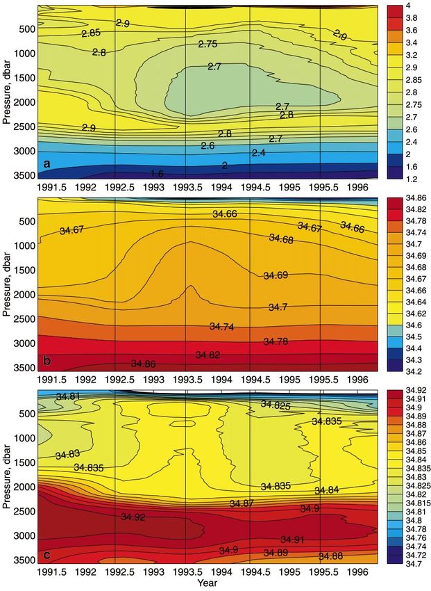
668                                JOURNAL OF PHYSICAL OCEANOGRAPHY                                                           VOLUME 32

FIG. 2. Sections of (a) potential temperature, (b) salinity, and (c) s1500 across the Labrador Sea along the AR7W section occupied in Jun
                                                                     1993.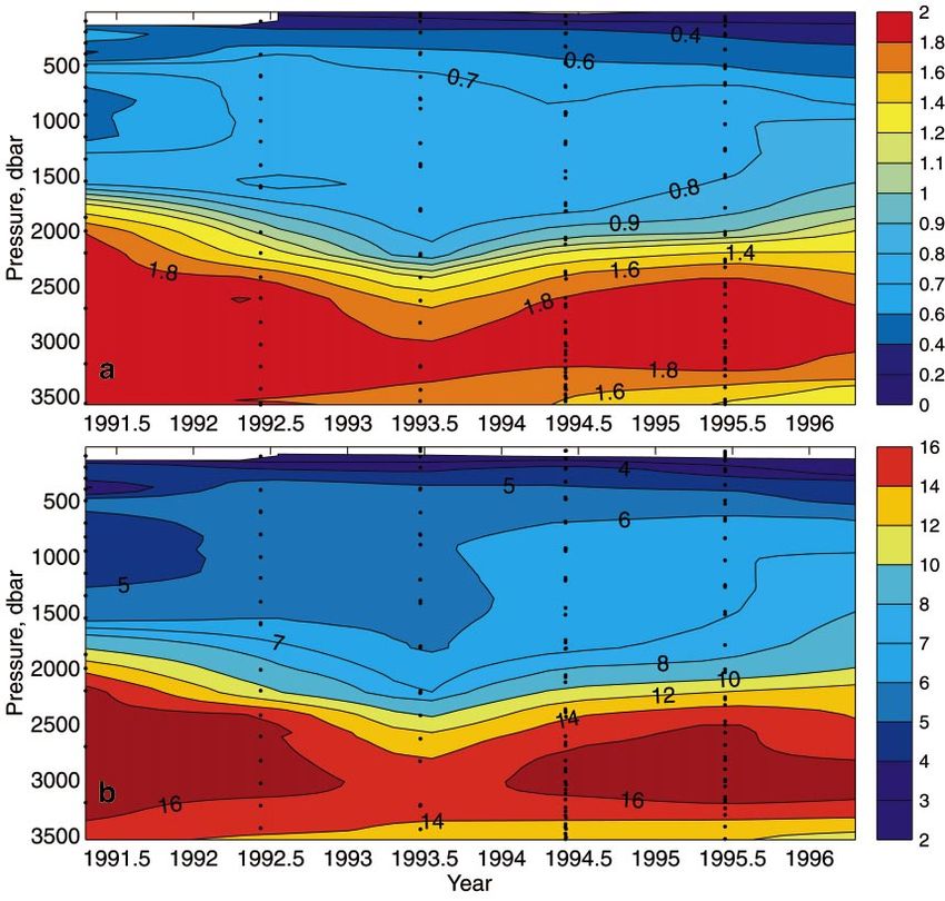
FEBRUARY 2002                                          KHATIWALA ET AL.                                                        669

                                                                        ently, the main source of tritium to the Labrador Sea is
                                                                        via the boundary currents transporting low-salinity wa-
                                                                        ter from the Arctic Ocean (Doney et al. 1993).
                                                                           Tritium decays to 3He with a half-life of 12.43 years
                                                                        (Unterweger et al. 1980), thus elevating the 3He/ 4He
                                                                        ratio in subsurface ocean waters above solubility equi-
                                                                        librium. In practice, a more useful quantity is tritiogenic
                                                                        3
                                                                          He, which is derived from the measured 3He concen-
                                                                        tration by correcting the latter for 3He in solubility equi-
                                                                        librium and for 3He originating from ‘‘excess’’ air (bub-
                                                                        bles). In this study, tritiogenic 3He will be reported in
                                                                        TU. 3He is a gas and its concentration in a water parcel
                                                                        tends to shift toward solubility equilibrium with the at-
                                                                        mosphere near the ocean surface; that is, the tritiogenic
                                                                        3
                                                                          He shifts toward 0 TU. By simultaneously measuring
                                                                        tritium and 3He we can compute the apparent ‘‘age’’ of
                                                                        a water parcel (e.g., Jenkins and Clarke 1976). In the
  FIG. 3. u–S plot for stations from the central Labrador Sea showing
the water mass structure described in the text. The three main water    absence of mixing, this age is the time elapsed since
masses, LSW, NEADW, and DSOW are indicated. The solid line is           the water parcel was isolated from the surface (e.g., by
a CTD cast from spring 1994 (58.28N, 50.98W). The gray dots rep-        convection). Such 3H– 3He ages (t th ) provide a first-or-
resenting all available data from the central Labrador Sea (see Fig.    der estimate of renewal rates and residence times. It
1 for locations) show the extent of hydrographic variability. Note      should be emphasized that the 3He concentration in the
that the data coverage is biased toward the 1964–74 period. Also
shown are contours of s1500 .                                           mixed layer is rarely in solubility equilibrium. Indeed,
                                                                        in regions with deep mixed layers (Fuchs et al. 1987)
                                                                        and rapid convection the finite gas exchange velocity
for ingrowth of tritiogenic 3He. The 3He ingrowth from                  (5–10 m day 21 ) can prevent t th from being reset to zero.
tritium decay was measured on a commercial VG 5400                      Furthermore, exchange with the boundaries, and in par-
mass spectrometer with a specially designed inlet sys-                  ticular with older recirculating waters, can also modify
tem (Ludin et al. 1998). Helium isotope samples were
                                                                        3
                                                                          H– 3He ages in a manner that complicates straightfor-
extracted using the same extraction system and mea-                     ward interpretation.
sured on a similar mass spectrometric system (MM
5400). Precision of the tritium data reported here is                   5. Distribution of transient tracers in the
62%, or 60.02 TU (tritium units), while that of the                        Labrador Sea
3
  He data is 60.05 TU (Ludin et al. 1998). The 3H– 3He
age in years was calculated by                                          a. 3H and 3He

                                 1                 2
                                         [ 3 He]                           Figure 4a shows the distribution of tritium across the
                   t th 5 t m ln 1 1                                    Labrador Sea. The surface-intensified boundary currents
                                          [ 3 H]
                                                                        with high tritium concentrations (4–7 TU) are clearly
where t m is the mean lifetime of tritium (17.93 yr).                   visible. This tritium is mixed laterally into the interior
                                                                        and then to depth during deep convection, thus pro-
                                                                        ducing the elevated tritium values of Labrador Sea Wa-
4. Overview of transient tracers
                                                                        ter.
   In this section we present a brief overview of the                      The distribution of 3He (Fig. 4b) mirrors that of 3H
transient tracers 3H and 3He. Tritium is produced nat-                  and clearly shows recently ventilated LSW, marked by
urally in the upper atmosphere, where it is oxidized to                 low excess 3He concentrations. The NEADW under-
HTO to participate in the hydrological cycle. Natural                   lying LSW is characterized by high [ 3He] and low [ 3H]
tritium concentrations in continental precipitation are                 values due to the long transit time from the eastern
;5 TU [Roether (1967): 1 TU represents a 3H/H ratio                     Atlantic. In contrast, DSOW, seen in the eastern part of
of 10 218 ], while those in surface ocean water are ø0.2                the section on the west Greenland slope, has relatively
TU (Dreisigacker and Roether 1978). This background                     low 3He and high 3H concentrations. Also interesting is
signal was masked by anthropogenic tritium produced                     the relatively high 3He values found on the Labrador
during atmospheric nuclear weapons tests, mainly in the                 shelf. Such elevated 3He concentrations are character-
early 1960s, and injected into the stratosphere. This el-               istic of Arctic waters, and are due to the large tritium
evated tritium concentrations in continental precipita-                 values coupled with the strong stratification, which in-
tion by two to three orders of magnitude, while those                   hibits vertical mixing and gas exchange, thus building
in Northern Hemisphere ocean surface waters increased                   up excess 3He (e.g., Schlosser et al. 1990). In the context
to about 17 TU (Dreisigacker and Roether 1978). Pres-                   of the Labrador shelf, the 3He is likely transported from
670 JOURNAL OF PHYSICAL OCEANOGRAPHY VOLUME 32 FIG. 4. Sections of (a) 3H, (b) 3He, and (c) 3H– 3He age across the Labrador Sea along the WOCE AR7W section occupied in Jun 1993.
FEBRUARY 2002                                       KHATIWALA ET AL.                                                               671

  FIG. 5. A schematic of the 2D numerical model (horizontal resolution 40 km, vertical resolution 87 m, time step 4320 s) showing its
                  various components. Also shown are the S and u profiles to which the lateral boundary is relaxed.

farther north. For example, Top et al. (1981) have noted             in a simple numerical model using idealized tracer
high subsurface 3He concentrations in Baffin Bay, and                boundary conditions. The model used here is two-di-
it is possible that the 3He observed on the Labrador                 mensional, formulated in cylindrical coordinates, and
shelf was transported in the Labrador Current from Baf-              based on the model described in Visbeck et al. (1997).
fin Bay.                                                             A schematic of the model is shown in Fig. 5. Since, to
                                                                     first order, the distribution of various properties is sym-
                                                                     metric about the central Labrador Sea, the Labrador Sea
b. 3H–3He age                                                        can be modeled as an azimuthally symmetric cylinder.
   Figure 4c shows the distribution of 3H– 3He age (t th ).          In the context of the numerical model, the domain is
Not surprisingly, LSW shows the lowest t th (4–6 yr),                thus a radial section across this cylinder.
consistent with its recent ventilation. The next oldest                 The model solves the linearized momentum equations
water mass in the Labrador Sea is DSOW (12–14 yr),                   in the hydrostatic, geostrophic, and Boussinesq limits.
followed by NEADW (16 yr).                                           The ocean model is forced by surface fluxes of buoy-
   It should be emphasized that t th is a rather crude               ancy. The surface heat fluxes are determined by a prog-
measure of ‘‘age’’ and caution must be exercised in its              nostic atmospheric boundary layer model (Seager et al.
interpretation. Indeed, in the presence of mixing a water            1995) coupled to the ocean model’s sea surface tem-
parcel cannot be assigned a single age but must instead              perature. The boundary layer atmospheric temperature
be characterized by an age distribution or distribution              and humidity are specified over land but vary over the
of transit times (Holzer and Hall 2000). However, as                 ocean according to an advective–diffusive balance sub-
shown by Khatiwala et al. (2001), tracer-derived ages                ject to air–sea fluxes. All other boundary conditions
(such as t th ) are weighted toward the leading part of the          such as the shortwave radiation, cloud cover, wind
transit-time distribution and can accordingly be fruit-              speed, and wind vector are specified at each grid point
fully interpreted and used. To better understand the be-             with monthly resolution. The prescribed monthly mean
havior of transient tracers in a highly variable environ-            air temperature and humidity are based on monthly
ment with relatively short timescales, such as the Lab-              mean meteorological data (collected between 1935 and
rador Sea, we have performed a series of simulations                 1995) from weather stations (Cartwright and Hopedale)
672 JOURNAL OF PHYSICAL OCEANOGRAPHY VOLUME 32
on the Labrador coast. The predominantly northwesterly
(cyclonic) winds justify the use of data from the Lab-
rador coast rather than from the West Greenland coast.
Monthly mean values for other variables were derived
from da Silva et al. (1994).
Tracers in the model are restored to prescribed values
at the lateral boundaries (Fig. 5). This is necessary be-
cause the ocean model has solid boundaries, and surface
fluxes of tracers (e.g., heat and freshwater) must be bal-
anced by sources or sinks elsewhere. In the Labrador
Sea, surface heat loss and freshwater input are balanced
by the convergence of heat and salt mixed in from the
warmer and saltier boundary currents. In the model, this
interaction with the large-scale circulation is represented
by means of relaxation boundary conditions at the pe-
riphery. These restoring boundary conditions (Fig. 5)
and the relaxation timescale (;4 months) were derived
by minimizing the weighted sum of the square of the
differences between model and observed variables [for
details see Khatiwala (2000)]. The model removes in-
stabilities created by surface forcing by a simple con-
vective adjustment scheme that mixes adjacent cells in
the vertical until the water column is stable. Transport
of tracers by eddies is parameterized by the Gent–
McWilliams scheme (Gent and McWilliams 1990; Vis-
beck et al. 1997) using an exchange coefficient, k, of FIG. 6. Time series (from top to bottom) of u, S, 3H, 3He, and t th
400 m 2 s 21 . Exchange of 3He between the ocean mixed simulated in a numerical model at three different depths (300, 500,
layer and atmosphere is parameterized in terms of a gas and 1500 m). No flux boundary conditions were imposed on 3H and
3
He at the sidewall.
exchange velocity. The gas exchange velocity for 3He
(y he ) in cm h 21 is computed following Wanninkhof
(1992): convection cools and freshens subsurface waters. Sub-
0.39w 2 sequently, u and S increase due to exchange with the
y he 5 , warmer and saltier boundary waters. The simulated con-
ÏSc/660 centrations of 3H, 3He, and calculated t th are shown in
where w is the surface wind speed and Sc(T) is the the bottom three panels of Fig. 6 at 300, 500, and 1500
Schmidt number for 3He at temperature T (in 8C) cal- m. Both 3H and 3He (and the calculated t th ) undergo a
culated as strong seasonal cycle as a result of the winter deepening
and subsequent shoaling of the mixed layer. It is sus-
Sc 5 410.14 2 20.503T 1 0.531 75T 2 2 0.006 011 1T 3 . pected that this strong seasonality is in part due to the
The flux of tritiogenic 3He out of the ocean is then given crude nature of the convective adjustment scheme em-
by y he [ 3He]/Dz where 3He is the surface concentration ployed, although no observations exist to demonstrate
and Dz is the thickness of the surface grid box. this. During winter, subsurface 3H concentrations are
In each of the simulations discussed here, the model elevated, while 3He is lost to the atmosphere. Conse-
was ‘‘spun up’’ for 30 years before initializing any pas- quently, the 3H– 3He age at 1500 m decreases from 3 yr
sive tracers. Thereafter, the model was integrated for an to ,2 yr. Following wintertime convection, the 3H– 3He
additional 70 years. Only the last two years of the sim- age starts increasing. The modeled mean 3H– 3He age at
ulation will be shown. The maximum depth of convec- 1500 m is ;2.5 yr, considerably less than the observed
tion was 2300 m. In the first experiment 3H was strongly (in June) age of 4–6 yr.
relaxed at the surface to 1 TU with a timescale of 0.2 While a detailed comparison between model and ob-
days, while 3He was allowed to approach solubility servations is obviously not very meaningful, we believe
equilibrium via gas exchange. The model produced typ- this difference in age is significant. One possibility is
ical winter gas exchange rates of 10–12 m day 21 . Both that lateral exchange with the relatively old waters along
3
H and 3He were subject to no-flux boundary conditions the boundaries of the Labrador Sea could affect the 3H
at the lateral wall. The modeled u and S variations in and 3He concentrations, resulting in higher observed
the convecting ‘‘interior’’ are shown in the top two pan- ages. To examine the influence of lateral mixing on 3H–
els of Fig. 6 at 300, 500, and 1500 m. There is a fairly 3
He age a second experiment was performed with more
robust seasonal cycle in u, which is also seen in the realistic lateral boundary conditions imposed on 3H and
observations (Lazier 1980; Lilly et al. 1999). Winter 3
He. At the surface, 3H was restored to observed values,FEBRUARY 2002 KHATIWALA ET AL. 673
salinity cycle (Lazier 1980). In this section we examine
this annual salinity signal. Previous work (e.g., Lazier
1982; Myers et al. 1990; Khatiwala et al. 1999) has
focused on freshwater sources to the Labrador shelf and
further downstream. Here we will synthesize the results
of earlier studies in the context of understanding the
freshwater inventory of the central Labrador Sea, and
systematically construct a freshwater budget in terms of
available sources. We begin by reviewing the freshwater
balance on the shelves.
a. Freshwater sources to the Labrador shelf
Recent work by Loder et al. (1998) using hydro-
graphic data and Khatiwala et al. (1999) using oxygen
isotope (d18O) measurements has examined the fresh-
water sources to the Labrador Sea. In particular, with
the available d18O data Khatiwala et al. (1999) con-
cluded that high-latitude rivers dominated by Arctic run-
off are the primary source of freshwater to the Labrador
shelf. This freshwater is transported into the Labrador
Sea via two pathways: the East–West Greenland Cur-
rents carrying low-salinity waters out of Fram Strait and
the Baffin Island–Labrador Currents linking the Arctic
Ocean to the Labrador Sea via the Canadian archipelago,
FIG. 7. Time series (from top to bottom) of u, S, 3H, 3He, and t th Baffin Bay, and Davis Strait (Fig. 1). Consistent with
simulated in a numerical model at three different depths (300, 500, hydrographic observations (Lazier and Wright 1993;
and 1500 m). 3H and 3He were restored to observations at the sidewall. Loder et al. 1998), the isotope data suggested that the
latter pathway involving the Canadian archipelago pre-
dominates. The pervasive influence of sea ice on the
while 3He was subjected to gas exchange as before. Labrador shelf was also documented. The importance
More importantly, both 3H and 3He were restored to of Arctic runoff is also seen in tritium data (Khatiwala
‘‘observations’’ at the sidewall on a timescale of ;4 2000).
months. Just as for temperature and salinity these re-
storing conditions are a crude attempt to represent the
boundary currents. The results of this experiment are b. Annual cycle of salinity in the Labrador Sea
shown in Fig. 7. The resulting 3H– 3He age at 1500 m As a first step, we have constructed a mean annual
is now much greater. This suggests that the 3H– 3He age cycle of salinity in the central Labrador Sea using data
is determined by a number of factors, such as intensity collected between 1964 and 1974 at Ocean Weather Ship
of convection, the extent to which the 3H– 3He age is (OWS) Bravo (568N, 518W), which was occupied in
reset by gas exchange, and mixing with ambient waters nearly all months during that period. We have not used
with different tracer concentrations. data from other years because in most years only a few
months were sampled at best. This poor coverage would
be less of a problem but for the presence of long-term
6. Freshwater sources to the central Labrador Sea
trends in the data (Lazier 1995), which could potentially
The nonlinear equation of state for seawater implies influence the estimated annual cycle. Even during the
that salinity rather than temperature controls density 1964–74 period the observations show significant trends
(and hence stability) at the low temperatures character- (Lazier 1980). In particular, the 1960s and early 1970s
istic of the subpolar ocean. As a result, changes in fresh- coincided with the passage of the Great Salinity Anom-
water supply have the potential to impact deep convec- aly (Dickson et al. 1988), weak atmospheric forcing,
tion. For example, the period of weak convection in the and moderate convective activity. To remove these
Labrador Sea during the late 1960s and early 1970s trends from the data a simple procedure was followed.
(Lazier 1995) has been linked to anomalously fresh- A mean profile of salinity was constructed for each cal-
waters in the subpolar North Atlantic (Dickson et al. ender month between 1964 and 1974. Next, at each
1988), and in particular on the West Greenland and Lab- pressure level interpolation was performed in time to
rador shelves. It should be remembered that these low fill in the few missing months. A first-guess seasonal
frequency fluctuations in the salinity of the near-surface cycle was then estimated from the resulting gridded
Labrador Sea are in fact superposed on a large annual field. To detrend the data, the estimated annual cycle at674 JOURNAL OF PHYSICAL OCEANOGRAPHY VOLUME 32
would be transported south in the Labrador Current and
laterally mixed into the interior. Regardless of the source
of the freshwater, in the absence of a mean advection
into the interior of the Labrador Sea, eddy exchange
appears to be the only plausible mechanism for the
freshwater flux. An alternative is for sea ice to drift into
the central Labrador Sea and then melt, but the available
d18O data suggest that this is not a significant mechanism
(Khatiwala et al. 1999).
It should be noted that our estimate of the seasonal
cycle is based on a period of low surface salinity in the
Labrador Sea (Dickson et al. 1988; Lazier 1995) and
weak convection. In years with more robust convection
near-surface salinity in winter may well be higher. For
example, in late February 1997 the salinity of the (well
mixed) upper 100 m was typically .34.8 psu (Pickart
et al. 2002). By mid-May of that year the salinity in the
central Labrador Sea was ;34.7 psu. No data are avail-
able from later in the year to assess the amplitude of
the seasonal cycle in recent years.
c. Sources of freshwater
An important question (Lab Sea Group 1998) is the
contribution of sea ice melt to the seasonal freshening
FIG. 8. Seasonal cycle (from top to bottom) of salinity in the central in the central Labrador Sea. The salinity data presented
Labrador Sea (upper 100 m) and on the Labrador shelf (upper 100 above do not directly identify the source of the fresh-
m) (Lazier 1982), and sea ice area on the Labrador Shelf, in Baffin
Bay, and in Hudson Bay. water, but the timing of the salinity minimum strongly
hints at sea ice meltwater being the dominant source.
To begin, consider the freshwater flux implied by the
each pressure level was subtracted from the correspond- salinity data. To produce the March–September fresh-
ing field and the residual smoothed with a 13-month ening in the central Labrador Sea requires ;60 cm of
boxcar filter to retain interannual variations. This freshwater, or a mean freshwater flux over that period
smoothed residual was next subtracted from the original of 11 mSv (mSv [ 10 3 m 3 s 21 ). For this calculation we
gridded field to obtain a detrended field. The procedure have used a disk of radius 300 km to represent the
was repeated once more, but the results did not change ‘‘central’’ Labrador Sea and assumed that the value of
significantly. The annual cycle we discuss below is de- 60 cm derived mostly from observations at OWS Bravo
rived from the detrended, gridded values. is, in fact, representative of that area. Lazier (1980)
The top panel in Fig. 8 shows the annual cycle of obtains a value of 30 mSv by using a substantially larger
salinity in the central Labrador Sea averaged over the area, but it appears that his value was meant to apply
upper 100 m. The salinity signal below a few hundred to the entire Labrador Sea. In any event, this flux should
meters is weak and opposes the decrease in the upper be compared to the total freshwater transport of the
100 m. Evidently, there is a large decrease in salinity Labrador and West Greenland Currents [;200 and 30
between March and September, which corresponds to a mSv relative to S 5 34.8 psu, respectively (Loder et al.
change in salt content (over the upper 100 m) of ;220 1998)] as well as that produced by melting of sea ice.
kg m 22 , or a salt outflux over that period of 1.3 3 10 26 To estimate the freshwater contribution from melting
kg m 22 s 21 . Equivalently, assuming a mean surface sa- of sea ice we have computed the annual cycle of sea
linity of 34.5 psu, this implies an addition of 60 cm of ice area (Fig. 8) in Baffin Bay, Hudson Bay, and on the
freshwater between March and September to the upper Labrador shelf from satellite microwave observations
100 m, similar to the value calculated previously by of sea ice concentration. By assuming an ice thickness
Lazier (1980). Averaged over the upper 1500 m, how- of 2 m for Baffin Bay and Hudson Bay, and 1 m for
ever, the net change in salinity is negligible, approaching the Labrador shelf (Ice Climatology Services 1992) the
the measurement precision (Lazier, 1980). ice volumes were converted into a ‘‘discharge’’ rate.
As suggested by Lazier (1980), the salinity changes The peak (March–August average) discharge rates thus
in the upper 100 m cannot be explained by precipitation calculated are 19 (11) mSv for the Labrador shelf, 190
(;20 cm during summer). Instead, he attributed the sea- (110) mSv for Baffin Bay, and 335 (134) mSv for Hud-
sonal salinity decrease to runoff and sea ice meltwater son Bay. The maxima for sea ice melt in each of these
delivered into Hudson Bay (see below). This freshwater regions occurs in June. In addition to meltwater, riverFEBRUARY 2002 KHATIWALA ET AL. 675
TABLE 1. Freshwater volumes from various sources. observations (Fig. 8) the ice cover is greatly reduced
Volume by June. Finally, runoff along the Labrador shelf con-
Source (3 1011 m 3 ) tributes an additional 1 3 1011 m 3 between March and
Labrador shelf sea ice (Mar) 1.6 September.
Baffin Bay and Davis Strait sea ice (Mar) 16 Having looked at the sources, it is useful to compute
Hudson Bay sea ice (Mar) 20 the volume of freshwater required to produce the ob-
Davis Strait ice drift (annual) 11 served freshening in the Labrador Sea. For the central
Labrador shelf ice drift (annual) 3 Labrador Sea we require 60 cm or 1.7 3 1011 m 3 of
Davis Strait ice drift (Mar–Jun) 5.6
Labrador shelf ice drift (Mar–Jun) 1.4 freshwater between March and September. On the Lab-
Labrador shelf runoff (Mar–Sep) 1 rador shelf the mean salinity (upper 200 m) changes by
Labrador shelf (top 200 m) required freshwater 7 ;0.75‰ between March and August (Lazier, 1982),
Central Labrador Sea (top 100 m) required 1.7 requiring an addition of nearly 4.6 m of freshwater.
freshwater
Integrated over the entire shelf (width ;150 km and
length ;1000 km), this requires the addition of 7 3
1011 m 3 of freshwater between March and August. Over
runoff along the Labrador coast is about 5 mSv, while the entire Labrador Sea the seasonal freshening requires
that into the Hudson Bay drainage area has a peak dis- the addition of ;9 3 1011 m 3 or 900 km 3 of freshwater.
charge rate (in June) of ø60 mSv (Inland Waters Di- All estimates are summarized in Table 1.
rectorate 1991). Undoubtedly, some of the sea ice ex- Clearly, although we have not included the contri-
isting at the beginning of the melt season is exported bution from runoff, Hudson Bay emerges as the largest
out of the region and will be lost as a freshwater source. potential source of freshwater. However, there is some
Consider now the timing of the salinity minimum in debate as to the importance of Hudson Bay sea ice melt-
the Labrador Sea. The salinity minimum on the Lab- water and runoff to the Labrador Sea. For example,
rador shelf occurs in July–August (Fig. 8) (Lazier 1982), Lazier (1980) suggests that the freshening in the Lab-
while that in the central Labrador Sea occurs in Sep- rador Sea can be explained by Hudson Bay sources,
tember. The obvious explanation for this timing is the while Lazier and Wright (1993) find evidence for the
seasonal melting of sea ice in the region, but we also dominance of Baffin Bay. The latter view is also re-
need to account for the export of sea ice out of the flected in the freshwater estimates made by Loder et al.
region. At this point it is more convenient to compare (1998). Furthermore, a lag-correlation analysis (Myers
the volume of available freshwater sources. Since we et al. 1990) shows that runoff into Hudson Bay has the
are interested in the summer freshening we first calculate most negative correlation with the salinity off New-
the amount of freshwater available in the form of sea foundland (downstream of the Labrador shelf ) at a lag
ice at the beginning of the melt season. This is reported of 9 months. Thus, the runoff pulse from Hudson Bay
in Table 1 for the Labrador shelf (1.6 3 1011 m 3 ), Baffin should reach the Newfoundland shelf in March. How-
Bay and Davis Strait (16 3 1011 m 3 ), and Hudson Bay ever, the salinity minimum off Newfoundland occurs in
(20 3 1011 m 3 ). Again, some of this ice, particularly on August–September, thus leading Myers et al. (1990) to
the Labrador shelf, will drift out of the region during conclude that Hudson Bay runoff does not contribute
the melt season and, while difficult to estimate just how significantly to the salinity minimum off Labrador and
much, an upper bound can be placed on the volumes Newfoundland. This inference is supported by data from
involved. Ingram and Prinsenberg (1998) estimate the a current meter in Hudson Strait where the surface sa-
annual mean sea ice export through Davis Strait to be linity reaches its minimum in November. Significantly,
equivalent to ;35 mSv of freshwater, while Loder et they find no consistent evidence of any relationship be-
al. (1998) estimate the sea ice drift along the southern tween sea ice melt into Hudson Bay and salinity off
Labrador coast (Hamilton Bank) to be ;10 mSv. This Newfoundland. This is surprising considering that the
represents an annual freshwater export of 11 3 1011 m 3 freshwater discharge from sea ice melt is at least twice
through Davis Strait and 3 3 1011 m 3 south of the Lab- as large as that produced by runoff. They attribute this
rador shelf (Table 1). However, we are more interested to the poor quality of sea ice data. In any event, the
in the ice export during summer. This can be crudely advective lags for both runoff and sea ice melt are likely
estimated as follows. The mean current velocity on the to be similar and, along with the salinity observations
southern Labrador shelf is ;10 cm s 21 (Lazier and from Hudson Strait, the evidence strongly suggests that
Wright 1993), while that in Davis Strait is ;20 cm s 21 neither river runoff nor sea ice melt from the Hudson
(Ingram and Prinsenberg 1998). Assuming that the sea Bay region contributes substantially to the seasonal
ice tracks the surface currents, for which there is some freshening of the surface Labrador Sea. This leaves Baf-
evidence, the potential export of ice between March and fin Bay as the primary source of freshwater, as there is
June is ;5.6 3 1011 m 3 out of Davis Strait and 1.4 3 insufficient sea ice on the Labrador shelf to provide the
1011 m 3 across the southern Labrador shelf (assuming a necessary 900 km 3 of freshwater. It is supposed that
width of 200 km for both sections). These should be over the summer months some fraction of the existing
considered upper bounds because according to satellite 16 3 1011 m 3 of sea ice from Baffin Bay and Davis676 JOURNAL OF PHYSICAL OCEANOGRAPHY VOLUME 32
Strait will be exported south and melt on the Labrador depths, we will also discuss the variation of tracer in-
shelf, while some of it will melt in situ and be trans- ventories in different layers (delineated by isobars).
ported in the Baffin Island Current and onto the Lab-
rador shelf. Lazier and Wright (1993) estimate that the
a. Potential temperature (u) time series
seasonal freshening just south of Davis Strait is ;70%
of that on the Labrador shelf and suggest that this low- Figure 9a shows the evolution of u in the central
salinity water is then advected south, producing the ob- Labrador Sea between 1991 and 1996. Below 1000 dbar
served freshening on the Labrador shelf. This leaves us u showed a monotonic decrease between 1991 and 1993.
with ;4 3 1011 m 3 of freshwater (split evenly between (For reference, Fig. 9b shows the time evolution of
the Labrador shelf and the interior) unaccounted for, s1500 .) In particular, the mean u between 1000 and 1500
and from Table 1 we see that sea ice export through dbar (core LSW) decreased by ;0.18C in that period.
Davis Strait can reasonably explain the balance. Interestingly, between 1991 and 1992, the average u of
The estimates presented here, while rather crude, the underlying layer (1500–2000 dbar) decreased by
quantitatively support the idea that sea ice meltwater is ;0.158C while that of the 500–1000-dbar layer re-
the dominant cause of the large annual cycle in the mained virtually unchanged. This strongly suggests that
Labrador Sea, both on the shelf and the interior. It is the properties of LSW are determined in part by surface
important to note that, since we are only discussing the forcing and mixing with underlying waters. It is also
seasonal cycle, this conclusion does not contradict the clear that convection to successively deeper levels be-
results of previous studies that identify Arctic runoff as tween 1991 and 1993 had eroded the upper part of
the most important contributor to the average freshwater NEADW (2000–2500 dbar) so that its temperature de-
transport along the Labrador shelf. (Arctic runoff also creased by ;0.38C. The mean temperature of the water
spreads into the central Labrador Sea, as seen by high column between 150 and 2500 dbar decreased by
surface 3H values.) Finally, it is interesting to note that ;0.18C. If the central Labrador Sea is treated as a one-
the total sea ice exported south of the Labrador shelf is dimensional fluid column, then such a cooling would
nearly twice that present at the end of winter on the require a net heat loss of 15 W m 22 over the entire two
Labrador shelf. This is consistent with the d18O–S cal- year period. This number, however, should be compared
culations of Khatiwala et al. (1999), which imply that with an estimated mean heat loss over that 2-yr period
nearly 2 m of sea ice is formed annually on the Labrador of 110 W m 22 (Kalnay et al. 1996). [We note that,
shelf as opposed to a directly observed value of 1 m according to Renfrew et al. (2002), National Centers for
(Ice Climatology Services 1992). That is, the total vol- Environmental Prediction (NCEP) fluxes are somewhat
ume of ice produced on the Labrador shelf is nearly biased toward higher values.] Comparing the actual
twice that present at the end of winter. cooling with that expected from a heat loss of 110 W
m 22 (Fig. 10) implies that the convergence of heat into
the central Labrador Sea nearly balances the atmospher-
7. Interannual variability in the Labrador Sea
ic cooling. The relatively small net storage of heat points
In this section we report changes in hydrographic and to an efficient mechanism for exchange between the
transient tracers in the central Labrador Sea between boundaries and interior. Following the winter of 1994,
1991 and 1996 and relate this variability to changes in the temperature increased at all depths, a feature dis-
the convective regime. It has long been recognized that cussed later.
the formation of Labrador Sea Water is not a steady- It is also instructive to look at the time history of
state process, but exhibits significant low frequency var- atmospheric forcing. In the absence of any wintertime
iability. Previous studies, notably those by Lazier (1980, measurements of heat loss during that period, we use
1995), have documented variability in the hydrographic the reanalyzed diagnostic net heat flux from the National
properties of LSW on decadal timescales and related Center for Atmospheric Research (NCAR)–NCEP data
them to changes in convective activity. Here, we will assimilation project (Kalnay et al. 1996). Measurements
focus on interannual changes in both hydrographic prop- conducted during the Labrador Sea Deep Convection
erties as well as transient tracers (tritium and 3He) and Experiment (Lab Sea Group 1998) in February and
relate them to the history of convection in the 1990s. March of 1997 indicate that the diagnosed heat flux was
The tracer data will be presented as time–pressure somewhat higher than the measured values but did well
‘‘sections’’, which were prepared as follows. Between in accounting for the heat storage inferred from CTD
1991 and 1996, for every cruise, a mean profile of tracer casts. It should be kept in mind that the shipboard mea-
in the central Labrador Sea (see Fig. 1 for locations) surements were not synoptic, which makes it difficult
was constructed by linearly interpolating the data onto to directly test the accuracy of the diagnosed heat flux.
a uniform pressure grid. For u, S, and s1500 , the higher The upper panel in Fig. 11 is a time series of winter
resolution CTD data were used. Next, for each pressure [December–March (DJFM) mean] net heat loss in the
level, the data were linearly interpolated onto a uniform central Labrador Sea. Also shown for reference is a time
time grid to arrive at the gridded (in time and pressure) series of the winter (DJFM) index of the North Atlantic
tracer fields. For the purpose of inferring convection Oscillation (NAO) (Hurrell 1995) based on the differ-FEBRUARY 2002 KHATIWALA ET AL. 677
FIG. 9. Time–pressure sections of (a) potential temperature, (b) potential density anomaly ( s1500 ), and (c) salinity from the central
Labrador Sea. Vertical lines show when the data were collected (typically in Jun).678 JOURNAL OF PHYSICAL OCEANOGRAPHY VOLUME 32
between 1991 and 1993, whereas the temperature data
suggest a monotonic increase in the depth of convection.
These observations are consistent with the idea that the
interior of the Labrador Sea in essence integrates in time
the effect of atmospheric forcing, and thus responds
more slowly to the relatively more variable surface forc-
ing. This implies that convection in previous years pre-
conditions the water column for the following winter
(Marshall and Schott 1999).
b. 3He time series
Temporal evolution of [ 3He] (Fig. 12a) closely fol-
lows the temperature changes, with the tritiogenic [ 3He]
of the LSW layer (1000–1500 dbar) remaining nearly
FIG. 10. A comparison of observed (broken line) and expected constant, while that of the deeper layer (1500–2000
(solid lines) potential temperature in the 150–2500 dbar layer in the
central Labrador Sea. The observed cooling between 1991 and 1993 dbar) decreased by ;0.5 TU between 1991 and 1993.
implies an average heat loss of 15 W m 22 over that period. The The 3He concentration of the 2000–2500 dbar layer de-
predicted temperature curves for that period were computed by ap- creased even more dramatically by 1 TU. This reduction
plying the indicated heat loss to the water column. The average heat was followed by an increase in the mean [ 3He] of the
loss between 1991 and 1993 (estimated from NCEP reanalysis) is
110 W m 22 .
1000–2500 dbar layer between 1994 and 1996. The 3He
concentration of the 500–1500 dbar layer shows a slight
increase between 1991 and 1993, reflecting the balance
ence of normalized sea level pressures between Lisbon, between the (finite) rate at which tritiogenic 3He can
Portugal, and Stykkisholmur/Reykjavik, Iceland. The escape to the atmosphere during deep convection, and
modulation of heat flux in the North Atlantic by the mixing with underlying waters with higher tritiogenic
NAO is well documented (Lab Sea Group 1998; Dick- 3
He concentration. It is thus apparent that excess 3He
son et al. 1996) and will not be discussed further. The is a particularly sensitive indicator of the ventilation
atmospheric forcing does not increase monotonically process, but is not reset to zero by convection (Fuchs
FIG. 11. (top) The time series of mean winter (DJFM) net heat flux (solid line) in the central Labrador Sea from the NCAR–
NCEP reanalysis, and the winter index of NAO (broken line). (bottom) The time series of anomalies of sea ice extent on the
Labrador shelf from SSM/I data. Vertical bars are average winter (DJFM) anomalies.FEBRUARY 2002 KHATIWALA ET AL. 679
FIG. 12. Time–pressure sections of (a) tritiogenic 3He concentration and (b) 3H– 3He age in the central Labrador Sea.
Dots show the time (typically in Jun) and pressure at which samples were collected.
et al. 1987). In particular, mixing with underlying and ported by the time evolution of s1500 (Fig. 9b), which
surrounding fluid with higher 3He concentrations can shows a sharp shoaling of the deeper isopycnals between
complicate its interpretation. 1991 and 1993, and following winter 1993/94 a more
The time evolution of u and 3He can be used to re- gradual deepening of the isopycnals in the upper 2000
construct (qualitatively) the time history of deep con- dbar.
vection in the Labrador Sea in the 1990s. The 3He con- It is important to note that our inferred ventilation
centration can decrease by gas exchange with the at- depth during winter 1994/95 (,1000 m) is quite dif-
mosphere during deep convection. Alternatively, it can ferent from the value cited by Lilly et al. (1999), who
increase by in situ decay of 3H (at a rate of ;0.1 TU suggest that convection that winter penetrated to a depth
yr 21 for typical LSW 3H concentrations of 1.5 TU) or of 1750 m. This difference exists because our estimate,
by ‘‘excavation’’ of deeper layers (in particular, based on large-scale tracer budgets, refers to the depth
NEADW). Thus, it appears that there was increasing to which the ocean was ventilated, while that of Lilly
convection between 1991 and 1993 as the stratified up- et al. (1999), which is based on evidence of convective
per part of NEADW was eroded, followed by a reduc- plumes in a mooring record (May 1994–June 1995),
tion in convective activity in 1994. Thereafter convec- refers to the depth to which these convective plumes
tion was restricted to shallower depths and probably did penetrated. Given the large lateral variations in depth
not penetrate below 800 dbar. These inferences are sup- of convection (Lab Sea Group 1998; Lilly et al. 1999;680 JOURNAL OF PHYSICAL OCEANOGRAPHY VOLUME 32
shallower convection in 1994 (,2000 m). Convection
in 1994 was still sufficiently robust to mix down the
excess freshwater, thus reducing the salinity of the 150–
2000-dbar layer. As mentioned above, this robustness
might have been due to preconditioning of the water
column in previous years. After 1994, the data suggest
that convection was restricted to the upper 500–800 m.
As a result, the salinity of the upper layer decreased as
freshwater accumulated, while that of the deeper water
increased due to lateral mixing. This strong reduction
in ventilation is consistent with the heat flux time series
(Fig. 11), which shows that average winter heat flux in
1996 was less than half its 1993 value.
d. 3H–3He age (tth )
FIG. 13. Time series of average salinity (open circles) in the upper
150 dbar in the central Labrador Sea. Also shown (*) to illustrate Finally, we discuss the time series of 3H– 3He age (Fig.
the variability is the average salinity at individual stations. 12b). As was noted above, the 3H– 3He ages depend not
only on the intensity of convection (‘‘ventilation rate’’)
and entrainment of underlying older water, but also on
Pickart et al. 2002), it is likely that convective events mixing with recirculating waters in the boundary cur-
observed at a single location do not adequately capture rents. Furthermore, the modeled 3H– 3He age also un-
the ventilation of LSW as diagnosed from tracer bud- dergoes a substantial seasonal cycle, decreasing in win-
gets. ter and increasing through the remainder of the year,
both by in situ decay of 3H to 3He and by mixing with
the ambient and boundary fluid. Given these compli-
c. Salinity time series
cations, our interpretation of the tracer-derived ages as
While the amplitudes of salinity changes (Fig. 9c) are ‘‘ventilation’’ or ‘‘residence’’ times will be largely qual-
small relative to changes in u or 3He, they are consistent itative.
with the inferred history of convection described above. During the early 1990s, t th of LSW (1000–1500 dbar)
The onset of deeper convection in winter 1992 mixed increased from 5 yr in 1991 to 6 yr in 1993. This in-
down the fresher surface waters, thus reducing the sa- crease in t th occurred even as convection penetrated to
linity of the deep waters. The largest changes occur in greater depths. In this case, mixing with older waters
the 1500–2000-dbar (0.02 psu) and 2000–2500-dbar with higher excess 3He concentrations coupled with a
(0.05 psu) layers. Like u, the salinity in the 500–1500- finite gas exchange velocity shifted the t th toward higher
dbar interval remained constant due to the competing values. Between 1991 and 1993, t th of the 1500–2000-
influence of mixing down of fresher water and entrain- dbar layer decreased from ;9 to 6 yr, while the mean
ment of saltier water from below. As the convection t th of the 2000–2500-dbar layer decreased from 16 to
penetrated even deeper in 1993 (;2300 m), eroding into 8.5 yr. After 1994, t th shows a systematic increase below
the saltier NEADW, the salinity throughout the upper ø800 dbar and, as convection was restricted to pro-
2000 dbar increased. However, the mean salinity of the gressively shallower depths, a decrease in the upper 500
150–2500-dbar interval remained virtually unchanged. dbar. This latter result is consistent with the notion that
Lazier (1995) has also noted the opposite trends in sa- as the winter mixed layer becomes shallower, tritiogenic
linity in the deeper and shallower layers, especially dur- 3
He is lost more effectively.
ing periods of increasing convective activity, and sug- Between 1994 and 1996 the 3H– 3He age of the 1000–
gested that salt is conserved through vertical mixing. 2000-dbar layer changed by nearly 2 yr over that 2-yr
An interesting feature is the sharp decrease in the period. Furthermore, the increase in 3He between 1994
salinity of the upper layer in June 1993 (Fig. 13). As and 1996 is roughly 0.2 TU, which can be explained
discussed above, freshwater produced by melting of sea almost entirely due to tritium decay (tritium decays at
ice is sufficient to account for the observed summer roughly 6% per year; for typical LSW 3H concentrations
freshening in the Labrador Sea. Consistent with this, we decay will produce ;0.1 TU of tritiogenic 3He per year).
hypothesize that the strong atmospheric forcing in win- These data thus give the impression that this layer is
ter 1993 resulted in increased sea ice formation on the responding as a stagnant water body. However, as is
Labrador shelf (lower panel of Fig. 11). Subsequent clearly seen by the increase in u and S after 1994 of
melting of the sea ice would then increase the amplitude waters below ;1000 dbar (Fig. 9), this layer is not truly
of the seasonal freshening. stagnant and exchanges tracers with the boundaries both
It appears that the combined effects of excess fresh- via an eddy-induced circulation (see below) and iso-
water and moderate atmospheric forcing resulted in pycnal stirring by eddies.FEBRUARY 2002 KHATIWALA ET AL. 681
8. Role of eddies in the Labrador Sea
The time series presented above shows that the central
Labrador Sea exchanges heat and salt very efficiently
with the warmer and saltier boundary currents. In the
absence of Eulerian mean currents it is clear that eddies
must play an important role in this exchange process.
In a recent study, Khatiwala and Visbeck (2000) pro-
posed the existence of an eddy-induced ‘‘overturning’’
circulation in the Labrador Sea and estimated its
strength using hydrographic data. Here we provide ad-
ditional evidence in support of the proposed eddy-in-
duced circulation and discuss its implications in more
detail. We first review the notion of an eddy-induced
circulation.
a. The eddy-induced circulation in the Labrador Sea
FIG. 14. Schematic of eddy-induced circulation in the Labrador Sea
Guided by previous work (e.g., Gill et al. 1974; Gent from Khatiwala and Visbeck (2000). The schematic is superimposed
et al. 1995; Visbeck et al. 1997), Khatiwala and Visbeck on a potential density section (see inset map for position of section)
(2000) suggest that the combined effects of buoyancy across the Labrador Sea. The proposed circulation consists of a sur-
and wind forcing result in a buildup of available po- faced intensified inflow (y *s ), sinking motion in the interior (w*), and
tential energy (APE), which is then released via the an ‘‘outflow’’ at depth (y *d).
action of baroclinic eddies. They propose that this re-
lease of APE due to slumping of isopycnals drives an tiwala and Visbeck (2000) attribute the absence of a
eddy-induced ‘‘overturning’’ circulation that is an im- signal below 1000 m to weak convection during the
portant aspect of the adjustment process following deep 1964–74 period (Lazier 1995). This is probably rea-
convection. The strength of this circulation could be sonable, but we believe that in years of more intense
inferred from hydrographic data by assuming that away convection the eddy-induced circulation likely extends
from the mixed layer the eddy-induced circulation is deeper. Here we present indirect evidence for such a
adiabatic; that is, deep eddy-induced circulation in the central Labrador
]s u Sea.
1 u · =su 5 0, (1) The upper panel in Fig. 15 shows the s u across the
]t
Labrador Sea in June 1994, while the lower panel shows
where s u is the potential density anomaly and u the the s u in May of 1995. As discussed above, tracer data
velocity, which can be split into mean (u ) and time- suggest that convection in winter 1994 reached ;2000
varying or ‘‘eddy’’ (u*) components. The proposed m, while that in 1995 was restricted to the upper 800
eddy-induced circulation is illustrated in Fig. 14. m. Evidently, in both years the density between 1000–
Applying the above equation to a mean annual cycle 2000 m is very uniform. Next, note the changes in the
of s u in the central Labrador Sea (1964–74) and in- 27.77–27.78 kg m 23 s u layer. In 1994 there are strong
voking continuity, they infer a vertical eddy-induced horizontal gradients in the thickness of this layer, par-
velocity, w* ø 210 23 cm s 21 (;1 m day 21 ), a surface ticularly near the boundary. By the following year
intensified inflow velocity, y *s ø 0.5 cm s 21 , and an (1995) these gradients have been smoothed out and the
outflow velocity (at depth), y *d ø 0.1–0.2 cm s 21 . Note 27.78 isopycnal (for example) is noticeably flatter.
that a y *d of this magnitude implies an isopycnal ex- These changes are consistent with the notion that the
change coefficient k ; y *d L greater than 300–600 m 2 eddy-induced flow effectively transports fluid adiabat-
s 21 (L 5 300 km, half the basin width) and considerably ically so as to remove such gradients (Gent et al. 1995).
larger toward the surface. In the process mass is rearranged so as to reduce the
available potential energy. This interpretation of the
density changes can be quantified as follows. In the
b. Deep eddy-induced circulation
central part of the basin the 27.77 isopycnal moved
One drawback of the technique employed by Khati- down by ;100 m between 1994 and 1995, while the
wala and Visbeck (2000) to quantify the eddy-induced 27.78 isopycnal moved up by ;400 m, implying ver-
circulation is that below ;1000 m vertical gradients in tically convergent motion in the core LSW layer. The
density are extremely small, and thus vertical eddy-in- implied vertical velocity for the lower isopycnal is ;1
duced motion would not produce any local changes in m day 21 , of similar magnitude (but of opposite sign) to
density. Thus, their technique cannot detect eddy-in- that estimated by Khatiwala and Visbeck (2000). If we
duced motion in the homogeneous core of LSW. Kha- consider a small cylinder in the central Labrador Sea ofYou can also read