Real Estate Taxes and Home Value: Winners and Losers of TCJA

Working Papers                                                                                                    WP 20-12
                                                                                                                  April 2020
                                                                                                                  https://doi.org/10.21799/frbp.wp.2020.12

Real Estate Taxes and Home Value:
Winners and Losers of TCJA
Wenli Li
Federal Reserve Bank of Philadelphia Research Department

Edison G. Yu
Federal Reserve Bank of Philadelphia Research Department

ISSN: 1962-5361
Disclaimer: This Philadelphia Fed working paper represents preliminary research that is being circulated for discussion purposes. The views
expressed in these papers are solely those of the authors and do not necessarily reflect the views of the Federal Reserve Bank of
Philadelphia or the Federal Reserve System. Any errors or omissions are the responsibility of the authors. Philadelphia Fed working papers
are free to download at: https://philadelphiafed.org/research-and-data/publications/working-papers.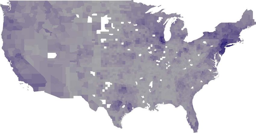

Real Estate Taxes and Home Value: Winners and Losers of TCJA

                                     Wenli Li and Edison G. Yu*

                                      First Draft: January 23, 2020

                                   This Draft Printed: April 1, 2020

                                                 Abstract
          In this paper, we examine the impact of changes in the federal tax treatment of local property
      taxes stemming from the implementation of the Tax Cuts and Jobs Act (TCJA) in January 2018
      on local housing markets. Using county-level house price information and IRS tax data, we find
      that capping the federal tax deduction of real estate taxes at $10,000 has caused the growth rate
      of home value to decline by an annualized 0.8 percentage point, or 15 percent, in areas where
      real estate taxes as shares of taxable income exceeded the national median. Additionally, these
      areas with a high real estate tax burden suffered from reductions in market liquidity after the
      reform. Fewer houses were transacted either in absolute numbers or as shares of total listings,
      houses stayed on the market longer before being sold, and more houses were listed with price
      cuts. Importantly, we find that the housing market slowdown was accompanied by declines in
      local construction employment growth as well as multi-family building permits. Furthermore,
      on net more people moved out of these areas after the reform. Finally, we show that the act has
      already had political consequences. In the 2018 midterm Senate elections, more voters voted for
      Democratic candidates in areas with high real estate tax burden than they did for Republican
      candidates.

         JEL codes: R0, R2, G1
         Keywords: real estate tax, home value, housing liquidity

* Wenli Li, Research Department, Federal Reserve Bank of Philadelphia, Email: wenli.li@phil.frb.org; Edi-
son Yu, Research Department, Federal Reserve Bank of Philadelphia, Email: edison.yu@phil.frb.org. We
thank seminar participants at the Federal Reserve Bank of Philadelphia and Princeton University for their
comments and suggestions. The views expressed in these papers are solely those of the authors and do not
necessarily reflect the views of the Federal Reserve Bank of Philadelphia or the Federal Reserve System. Any
errors or omissions are the responsibility of the authors.

                                                      1

1.     Introduction

     The Tax Cuts and Jobs Act (TCJA), which went into effect on January 1, 2018, made the most

significant changes in the federal tax treatment of homeownership since the Tax Reform Act of 1986.

Among the many changes in the act, itemized deductions of state and local taxes (SALT) from

federal income tax, previously uncapped, are now limited to $10,000 for individuals and married

couples filing jointly. This change undoubtedly affected different geographical areas differently as

households’ SALT obligation varies significantly with their residence. For instance, for the tax year

of 2016, Internal Revenue Service tax data indicate that the average ratio of real estate taxes to

adjusted gross income ranged from zero in Houston County, Georgia, King County, Texas, and

Hayes County, Nevada to over 5 percent in Putnam County and Rockland County in New York.1

For homeowners living in areas with high state and local taxes,2 the change directly lowered the

value of tax-exempt imputed income from owning their houses.

     In this paper, we provide the first nationwide analysis on the heterogeneous impact TCJA had

on U.S. residential housing value as well as other economic consequences over the period between

January 2018 and October 2019. The main part of our study tests how changes in the tax treatment

of homeownership in TCJA affected house prices across different geographical locations. It is

important to understand this impact because housing wealth constitutes almost half of American

household wealth and about 80 percent of the housing wealth is in owner-occupied units. Using

county-level house price data from Zillow, an online real estate data company, and a difference-in-

difference estimation method across time and space, we find that counties with high real estate taxes

relative to income had slower house price growth during the first 22 months after the implementation

of TCJA.

     In our analysis, we utilize several measures of local home value including median home value

per square foot, sale price, listing price per square foot and Zillow Home Value Index to fully take

advantage of the different strength of these measures in terms of their coverage and construction

methodology. We also calculate growth rates at both the (annualized) month-to-month frequency

and the year-to-year frequency to capture different price growth volatility over different horizons,
   1
     Note that in the IRS data, zero real estate taxes imply that no residents filed using itemized deductions or they
had zero property tax in the itemized deductions.
   2
     Local taxes are typically collected as property or real estate taxes.

                                                          2

as year-over-year growth rates typically exhibit less volatility than month-over-month growth rates.

Under our benchmark measure, annualized monthly growth rates of median home value per square

foot, we find that counties with real estate taxes relative to income in the top half of the nation

experienced a drop in home value growth rate of 0.8 percentage point per year or 15 percent during

the first 22 months after the implementation of TCJA. This is equivalent to $2,400 for the median

house in the high tax counties. The other measures generate a decline in house value growth rates

ranging from a low of 0.05 percentage point to a high of 2.6 percentage points.

       A number of events took place in and around 2018 besides the implementation of TCJA. For

instance, the Federal Reserve raised interest rates three times in 2017 and then another three

times in 2018 before lowering them three times in the second half of 2019. Mortgage rates rose in

response during most of our sample period, hurting areas with high house prices where households

likely need to borrow large amount of mortgages. Additionally, TCJA was first introduced in the

House in November 2017, two months before it was signed into law. As a result, households may

have preemptively responded to the proposal. To address the concern that these events may have

caused different areas to have different trends in house price growth prior to 2018, and, as a result,

invalidate our difference-in-difference estimation method, we introduce additional controls such as

lagged mean house value in our analysis. More important, we conduct placebo tests where we

assume the intervention occurred in the other months of our sample period than January 2018.

We find that our estimates are robust to the introduction of additional controls and there exist no

statistically significant price effects associated with these other dates in the placebo tests.

       Our main argument for constructing real estate tax burden, i.e., normalizing real estate taxes

paid by taxable income, to proxy for different location’s exposure to TCJA is to account for the

fact that households living in expensive areas also have higher income on average.3 It is true,

however, that TCJA imposes constraints on tax levels. We thus repeat our analysis using average

real estate taxes paid while controlling for taxable income as well as the other factors included in

the previous analyses. We find that counties with average real estate taxes paid in the top half

of the nation experienced a decline of 1.5 percentage points or 30 percent in house price growth

during that period.
   3
    In addition to the differences in statutory tax rates, our measurement of real estate tax burden captures differences
in property tax exemptions states offer to older homeowners and the disabled as well as property tax breaks for home
improvements and the installation of renewable energy.

                                                           3

To investigate the heterogeneous response within the local housing market, we further divide

the local market by its purchase prices relative to the area median and repeat our analysis using

the corresponding house price index from CoreLogic Solutions. We find that the negative impact

on house price growth rates was most felt within the medium range of the market. While the

most expensive segment of the local housing market also suffered after the tax reform, the positive

income effect it received from the reduction in income tax rates for high income brackets negated

the magnitude.

      Given that residential rental prices are typically closely tied to residential house prices, it is

likely that the slower house price growth transmits to the rental market and leads to slower rental

price growth. TCJA, however, adversely affects only homeowners while landlords can continue to

claim all SALT taxes as business expenses. In addition, TCJA added a generous new business

deduction for pass-through businesses which benefited small business owners such as landlords.

Indeed, our analysis reveals that the tax reform did not have a negative impact on local rent price

growth.

      Housing market liquidity affects households’ ability to buy and sell housing units. Asset prices

tend to decline when liquidity is poor. Using several proxies for local housing market liquidity and

the same difference-in-difference estimation technique, we find that, after TCJA, in areas with high

real estate taxes relative to income, fewer houses were sold both in absolute numbers and relative

to those listed, houses stayed on the market longer before being sold, and more listed houses had

price cuts. In other words, TCJA reduced housing market liquidity in areas with high real estate

tax burden. This deterioration in housing liquidity likely contributed to the severity of the decline

in local house price appreciation rates.

      Taken together, our analysis indicates that there were sizable slowdowns in local house price

growth in high tax areas after TCJA took effect. We next investigate whether these declines

had real economic consequences and how households have responded to its differential impact

across geographical regions. For real economic consequences, we focus on employment in the local

construction sector and building permits granted.4 Our study suggests that, after the reform,

growth rates in local construction sector employment slowed and building permits granted for

multi-family units also declined in areas with high real estate taxes relative to income. Given the
  4
      A building permit is the approval given by a local jurisdiction to proceed on a construction project.

                                                           4

sizable negative effects on house prices and real economic variables associated with TCJA, it is,

therefore, not surprising that less than two years after the implementation of TCJA, more people

have moved out of areas with high real estate tax burden after the reform relative to areas with low

real estate tax burden. This effect is more pronounced for individuals with a mortgage, a proxy of

their homeownership status. Furthermore, it is also not surprising that the act appeared to have

had political consequences. During the 2018 midterm Senate elections, the share of voters who

voted for Democratic candidates increased in areas with real estate tax burdens above the national

median. This result holds irrespective of the party affiliation of the incumbent candidate or the

Senate election results in 2016.

      The paper proceeds as follows. In the next section, we conduct literature review. In Section 3,

we summarize the changes in SALT deduction as a result of the TCJA and present a simple user

cost model. Section 4 describes the data. Section 5 investigates the differential impacts of the tax

reform on house price growth across different geographical areas. Section 6 studies the effects of

the tax reform on rental prices and house market liquidity. Section 8 explores other real economic

effects. Section 9 concludes.

2.      Literature Review

      Our paper is related to an extensive literature that investigates the effect of taxation on resi-

dential housing. Earlier seminar papers include Laidler (1969), Aaron (1972), and Rosen (1985),

who examine the efficiency losses of tax policy using Harbinger methods. Using an asset-market

approach, Poterba (1984) estimates that the coincidence of high inflation rates and the tax destruc-

tibility of nominal mortgage payments in the late 1970s and early 1980s accounted for as much as

a 30 percent increase in real house prices. Poterba (1991) and Poterba (1992) study the long-run

effect of the changes in tax policy toward housing in the 1980s (e.g., reductions in marginal in-

come tax rates and increases in standard deductions) and find the tax changes reduced attraction

of homeownership at high income levels and lowered after-tax rent benefits for landlords but had

muted effects on house prices.5 Capozza et al. (1998) assess the impact of income and property

taxes on house prices using a panel data for 63 metropolitan areas from 1970 to 1990. They find
  5
    Poterba (1991) suggests changes in income, construction costs and baby boomers coming of age may explain the
lack of the price declines in response to the 1980s reform that increased the user cost of homeownership.

                                                       5

that a cut in marginal federal income tax rates and the removal of the property tax deduction lower

house prices significantly with limited impact on homeownership rate or housing investment.

   More recently, using data from 1984 to 2007, Hilber and Turner (2014) find that state and

federal mortgage interest deduction only boosts homeownership of higher income households in

less tightly regulated housing markets. Davis (2019) studies the distributional impact of mortgage

interest subsidies and finds that average buyers at most incomes do not benefit from the mortgage

interest subsidies. As in our paper, Peach and McQuillan (2019) and Gilbukh et al. (2019) study

the impact of TCJA on housing. Peach and McQuillan (2019) focus on home sales between 2017Q4

and 2018Q3. They find evidence that changes in federal tax laws enacted in December 2017 have

contributed to the slowdown in housing sales, a finding we confirm in the paper. Using matched

CoreLogic Solutions MKS data from January 2010 to October 2018, Gilbukh et al. (2019) document

a narrowing in price/rent ratios between high- and low-tax states since the tax changes that started

taking effect at the beginning of 2018. In level terms, the ratios in high-tax, high-itemization areas

have stopped moving higher while the ratios in the rest of the country have continued to rise. Our

paper differs from theirs in that we use a national sample and difference-in-difference approach

that controls for other observables. In other words, we seek to isolate the effect associated with

the implementation of TCJA on the housing market from other factors such as interest rates and

local demand. Our results also suggest a narrowing in price-rent ratios between high-tax, high-

itemization areas and low-tax, low-itemization areas, but the narrowing came from the decline in

house price growth rates in the high-tax areas.

   In addition to the works cited above, in recent years researchers have used theoretical dynamic

models in the quantitative macroeconomic tradition to study these issues. Berkovec and Fullerton

(1992) find that the benefits to homeowners from the mortgage interest rate and property tax

deduction are small in a static general equilibrium model. In a dynamic model but focusing on

long-run steady state, Gervais (2002) and Chambers et al. (2009) also find that the elimination

of taxation of the imputed rental income from owner occupied housing and mortgage interest

deductions have small aggregate as well as distributional effects. Chatterjee and Eyigungor (2015),

however, find that the 2008 foreclosure crisis might have been smaller if mortgage interest payments

had not been tax deductible. Additionally, Sommer and Sullivan (2018) find much larger effects of

changing housing tax policies than the earlier research once house prices and rents are endogenized.

                                                  6

For example, eliminating the mortgage interest deduction causes house prices to decline and, hence,

increases homeownership and improves welfare. Rappoport (2018) builds an economic model that

features user cost and simulates the potential effect of TCJA on house prices. He finds that

simulated house prices decline an average of 2 percent across a sample of 269 metropolitan areas

with large dispersion ranging from as much as 7 percent to 0 percent. Our estimates are surprisingly

in line with the simulated findings in Sommer and Sullivan (2018) and Rappoport (2018).

3.       Homeowners and the Tax Treatment Before and After TCJA

     TCJA made significant changes to the federal income tax code for individuals and businesses.

As summarized in Peach et al. (2018), several provisions of the new tax law have altered the

tax treatment of individual homeownership in a number of ways. Among them, the new SALT

deduction cap is the most significant change. Itemized deductions of SALT, previously uncapped,

are now limited to $10,000 for singles and married couples filing jointly. The SALT deduction

provides a significant amount of savings for homeowners who itemize and pay a lot of real estate

taxes. For example, the average amount of real estate tax reported for tax filers who itemized in

2016 is about $3,800, which amounts to a $950 saving per year assuming a 25 percent marginal

federal income tax rate. The savings are even larger for households in areas with higher real estate

taxes.

     To take advantage of the SALT deduction, a tax filer has to itemize deductions. Since the tax

reform also increased the standard deduction substantially, the incentive to itemize decreased after

2018. For married couples filing jointly, the standard deduction increased to $24,000, almost double

the $12,700 figure in 2017. For individuals and heads of households, the deduction increased to

$12,000 and $18,000, respectively. Hence, capping the SALT deduction reduces the tax benefits of

owning a house.

     We use a simple model to describe effects of these changes on the tax benefits of homeownership.

To understand the implications of capping SALT deductions embodied in TCJA, we first review

the user cost of capital approach outlined in Poterba (1984) and subsequently adopted by many

other studies such as Himmelberg et al. (2005), Poterba and Sinai (2011), and Albouy and Hanson

(2014). Let ω denote the one-period cost of housing services from a house with real price of Q.

                                                  7

Before the implementation of the TCJA, the cost can be written as

           ω = [τp + ib (Q − m)/Q + im m/Q + δ − πH ] − τy [τp + im m/Q] × I[itemized],             (1)

where τy is the federal income tax rate; τp is the property tax rate; ib is the opportunity cost

of the fund; im is the mortgage interest rate; m is the amount of mortgage borrowed; δ is house

maintenance cost as a proportion of house value; πH is the expected house appreciation rate; and

I[itemized] is an indicator that takes value one if the household itemizes tax deductions. The terms

inside the first brackets of equation (1) represent the usual user costs of owning a house and the

remaining items in the equation represent the tax benefits of homeownership.

   It is important to bear in mind that the user cost of homeownership matters only if the home-

owner decides to itemize. Hence the tax benefit is equal to zero for tax filers not itemizing de-

ductions. But homeownership also makes a tax filer more likely to itemize deductions due to the

property taxes paid. For example, before the tax reform in 2017, the standard deduction for married

couples filing jointly is $12,700. So the indicator function takes the form

                          I[itemized] = I[τp Q + Ts + im m + X > 12700),                            (2)

where Ts indicates other state or local taxes, and X is all the other tax deductions. The larger the

size of property tax τp Q, the more likely a household itemizes and the higher the tax benefits as

illustrated in equation (1).

   The tax reform affects both equations above. First, for households who continue to find benefits

from using itemized deductions, the deductions become less generous due to the SALT deduction

cap. In equation (3), the property tax deduction is no longer unlimited, but capped by the difference

of $10,000 and Ts , other SALT excluding the real estate taxes that the tax filer is already paying:

 ω = [τp + ib (Q − m)/Q + im m/Q + δ − πH ] − τy [max(τp Q, 10000 − Ts , 0) + im m]/Q × I[itemized]. (3)

   Second, increasing the standard deduction limit to $24,000 and capping the SALT deduction in

2018 reduce a tax filer’s incentive to itemize. The indicator function in equation (4) is much less

                                                   8

likely to take the value one, holding SALT and other deductions fixed:

                      I[itemized] = I[max(τp Q + Ts , 10000) + im m + X > 24000)].                                (4)

       Hence, the tax reform reduces tax savings of user costs for homeowners in areas with higher real

estate taxes due to the new SALT cap, holding other things equal. If we assume that the housing

utility Qω is kept fixed before and after the tax reform, house prices Q fall as user cost ω increases,

particularly in places with higher real estate taxes.6

       It is important to note that other changes in the tax reform may directly and indirectly affect

the user costs that are not captured in the equations (1) – (4) for ease of exposition. For example,

the limit on the mortgage interest deduction for a married couple filing jointly has been reduced to

the interest on a maximum of $750,000 of acquisition indebtedness, down from $1,000,000 under

the old law. For individuals, the limit has also been lowered to $750,000. Spouses filing separately

each face a $375,000 limit. Compared with the SALT provision, this provision affects only new

home buyers after 2018. We control the effect of the new mortgage interest deduction cap in our

empirical analysis explicitly in section 5.1.7 TCJA also lowers the federal income tax rates for many

households and this change lowers the tax savings of homeownership due to fewer federal taxes paid

in the first place. In our empirical section 5.1, we explicitly address the potential impact of the tax

reform on households with different income levels.

4.       Data and Summary Statistics

4.1.      Housing

       Our housing related data mainly come from Zillow Group, Inc., an online real estate database

company. These include median home value per square foot (calculated by taking the estimated

home value for each home in a given region and dividing it by the home’s square footage), median

list price per square foot (median of list prices divided by the square footage of a home), median
   6
     One justification for this assumption is that rental markets are competitive. We also show that the rental prices
in high tax places are not disproportionally more affected by the tax reform in Section 6.
   7
     TCJA also suspends the deduction for interest paid on home equity loans and lines of credit when they are used
for something other than substantial improvement of their home. This provision is applicable regardless of when the
home equity debt had occurred.

                                                          9

sale price, Zillow home value index,8 home sales (the number of homes sold for the given time),

listings with price cut (the percentage of current for-sale listings on Zillow with a price cut), and

days on the market (the median days on market of homes sold including foreclosure resales). We

further construct sales to listings ratios by dividing total number of home sales by total number of

listings for the given time.

    Home sales are arms-length transactions of single-family, condominium and cooperative prop-

erties. They include real-estate-owned sales as well as auctions, but exclude bank takeovers of

foreclosed properties, title transfers after a death or divorce and non arms-length transactions. A

transaction date is defined as the closing date recorded on the county deed. The data are publicly

available at Zillow Research.

    House price indices for different housing market segments come from CoreLogic Solutions, Inc.

CoreLogic Solutions House Price Indices are repeat sales indices that match house price changes

on the same properties in the public record files. CoreLogic Solutions computes separate indexes

by geographical areas and by purchase prices. In particular, CoreLogic Solutions constructs four

purchase price tiers depending on whether the home sold for less than 75 percent of the area median

price, for between 75 percent and 100 percent of the area median, for between 100 percent and 125

percent of the area median and for more than 125 percent of the area median.

    For mortgage information at the time of application, we make use of the Home Mortgage Disclo-

sure act (HMDA). HMDA records the vast majority of home mortgage applications and approved

loans in the U.S. for both purchases and mortgage refinances. The data provide, among other

things, mortgage applicants’ application status, income, purpose of borrowing, occupancy type,

and, importantly for the purpose of this paper, loan amount. We calculate the share of applica-

tions whose mortgages are above $750,000. These are the people who would have been affected by

the change in the cap in mortgage interest deductions in TCJA had TCJA been implemented that

year.
    8
      Zillow home value index draws on Zestimates calculated on more than 100 million U.S. homes, including new
construction homes and/or homes that have not traded on the open market in many years. To calculate a Zestimate,
Zillow uses an algorithm that incorporates data from county and tax assessor records and direct feeds from hundreds
of multiple listing services and brokerages. The Zestimate accounts for variables like: home characteristics including
square footage, location or the number of bathrooms; unique features like hardwood floors, granite counter tops
or a landscaped backyard; on-market data such as listing price, description, comparable homes in the area and
days on the market; and off-market data — tax assessments, prior sales and other publicly available records. See
https://www.zillow.com/zestimate/ for more details.

                                                         10

4.2.     Tax

       The individual income tax data come from the IRS for the year 2016, which is tabulated using

individual income tax returns (Forms 1040) filed with the IRS during a calendar year. The data

include adjusted gross income, total number of returns, number of returns with itemized deductions,

total itemized deductions amount, state and local income tax amount, and real state tax amount.

With these data, we can calculate the indexes that capture the exposures of an area to TCJA: the

average real estate tax to income ratio per tax return and the average adjusted gross income per

tax return.9

4.3.     Other

       We obtain additional county-level information from various sources: unemployment from the

Bureau of Labor Statistics, and total employment from the quarterly Census of Employment and

Wages (QCEW). We also calculate the county-to-county migration flow using the FRB New York

Consumer Credit Panel/Equifax. The credit panel is a nationally representative 5 percent random

sample of all individuals with a Social Security number and a credit report (usually aged 19 and

over) drawn from Equifax credit report data.10 Finally, we obtain the 2016 and 2018 county-level

Senate general election information from Princeton University.11

4.4.     Summary Statistics

       Our real estate data span January 2015 to October 2019. We merge the real estate data with

the 2016 tax data by county. For our baseline sample, we have an unbalanced panel with 3,079

unique counties. Table 1 presents the summary statistics of the main variables and the number of

observations available for the associated variables.

       According to Table 1, between January 2015 and October 2019, the annualized monthly median

growth rate for house value per square foot averaged 5.2 percent. However, the variance of the
   9
     Note that the tax data do not represent the full population of a given region because many individuals are not
required to file an individual income tax return. Additionally, tax returns filed using Army Post Office (APO) and
Fleet Post Office addresses, foreign addresses, and addresses in Puerto Rico, Guam, Virgin Islands, American Samoa,
Marshall Islands, Northern Marianas, and Palau are excluded.
  10
     The credit panel is a nationally representative 5 percent random sample of all individuals with a Social Security
number and a credit report (usually aged 19 and over) drawn from Equifax credit report data.
  11
     Data source: https://libguides.princeton.edu/elections/us#s-lg-box-1612393.

                                                         11

growth rate was large. The top 5 percent of the counties had a growth rate of 23 percent while the

bottom 5 percent of the counties had a price decline of 13 percent. In terms of levels, the median

house value per square foot averaged $109 and the median was $82. The number of house sales

also differed significantly across counties with an average of 240 and a median of 57. About 13

percent of the listings had a price cut. On average, a sale occurred after staying on the market for

3 months. Over 95 percent of the houses were sold after the listing during our sample period.

   The size of the county as measured by the number of tax returns filed varied over time and

across the counties with a mean of roughly 76,000 and a median of about 20,460. Real estate taxes

as fractions of total gross income ranged from under 0.76 percent to almost 5 percent. Different

counties had different income distribution. In the poorest counties, over 3 percent of the filers had

adjusted gross income less than $1,000. By comparison, in the richest counties, more than 7 percent

of the filers had gross adjusted income above $200,000. In 2016, very few counties had new home

buyers who took out mortgages over $750,000.

   Finally, we present summary statistics for alternative house price growth rate measurement.

Though these measurement had similar annualized mean growth rates, the variances were much

larger when measured month over month than year over year. This is particularly true for median

sale price and median list price per square foot. Not surprisingly, given its methodology, the Zillow

house price index is the smoothest of all the measurement.

4.5.   The Distribution of Real Estate Tax Burden in 2016

   We do not directly observe real estate taxes each household faces. However, we do observe at

the county level the average share of real estate taxes to taxable income for those who itemize

their tax deductions, which we proxy as a county’s exposure to changes in the tax treatment of

real estate taxes in TCJA. We discussed in the last subsection that the real estate tax burden thus

constructed varies between 0.4 percent to almost 5 percent. In Figure 1, we graph the geographical

distribution of the tax burden. Areas with darker shades of blue are areas that have higher real

estate tax burden. As expected, these areas are concentrated in the East Coast such as Boston,

New York City, and the states of Connecticut and New Jersey; the West including major cities

in California and Portland in Oregon; and a few areas in central Texas and in Chicago near Lake

Michigan.

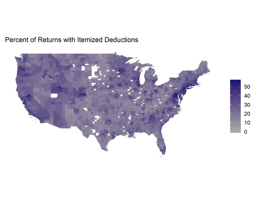
                                                 12

In Figure 2, we present the map which charts the distribution of the fraction of tax filings with

itemized deductions. Not surprisingly, areas with high real estate tax burdens are also areas that

have large fraction of tax returns with itemized deductions. Given their relatively moderate income

level, however, areas in the Midwest and Southeast, despite having large fractions of tax filings with

itemized deductions, do not have large tax burdens.

5.     Real Estate Taxes and House Prices

     In this section, we use a difference-in-difference approach to examine how the implementation

of TCJA affected local residential house prices through its changes in the deductibility of local real

estate taxes. As discussed earlier, because the limit TCJA imposed on SALT deduction in federal

taxes is uniform across the country, we expect the impact to be most felt in counties where the real

estate tax burden is already high.

     In Figure 3 panel (a), we chart the year-over-year growth rates of house value per square foot

for high real estate tax versus low real estate tax areas. We use the per square foot measure because

it controls for the house size in a county. High real estate tax areas include counties with average

real estate tax relative to taxable income, i.e., real estate tax burden, above the median of the

country in 2016. Low real estate tax areas include counties with average real estate tax burden

below the median of the country in 2016. We see that the two groups exhibit similar trends in home

value growth rates prior to the implementation of TCJA. After the reform, however, the two groups

demonstrate markedly different growth patterns, with the high tax burden areas experiencing much

slower house value growth relative to the low tax burden areas. This phenomenon is more evident

in Figure 3 panel (b) where we chart the growth rates of high tax group minus those of the low tax

group. The difference exhibits a prominent downward trend after January 2018, the date TCJA

became effective, indicating that home values grew slower in higher tax counties relative to lower

tax counties. Before January 2018, there was no obvious trend of the difference.

     As the next exercise, we divide the counties into five groups according to their real estate tax

burden. In Figure 3 panel (c), we chart the difference in year-over-year home value growth rates

of the top quintile and the bottom quintile. Prior to TCJA, there did not appear to be a trend in

home value growth rates between the two groups. After TCJA, however, home value per square

                                                  13

foot grew much faster for the bottom quintile than it did for the top quintile, leading to a drastic

decline in the difference of the growth rates.

   Formally, Table 2 reports the results of the difference-in-difference regressions. In the regres-

sions, we measure house price growth rates as annualized monthly growth rates of home value

per square foot. Column (1) estimates that the implementation of TCJA reduced the house price

growth rates of counties with above median real estate tax burden by 3.5 percentage points relative

to counties with below median real estate tax burden. House price growth is serially correlated and

often exhibits significant seasonality. Hence, column (2) controls for twelve lags of the house price

growth rates. The effects are smaller but remain negative and statistically significant.

   While the difference-in-difference approach has the advantage of being simple and straightfor-

ward, we need to address concerns of our identification strategy. The first concern is related to

confounding factors. The results in Table 2 can be spurious due to confounding events that oc-

curred at the same time as the tax reform that also have differential impacts on house value growth

in high and low tax counties. For example, the tax reform made significant changes to the federal

income tax brackets. Since levels of income are correlated with real estate taxes at the county level,

the negative coefficients we see in the regression can be because counties with higher income had

slower growth of home value due to the changes in the income tax brackets. Section 5.1 addresses

these concerns by including various controls to ensure no spurious regression results.

   Second, the difference-in-difference approach requires the parallel trend assumption. House

price of high and low real estate tax counties need to have a similar trend absent of the tax reform.

We test this assumption by using two separate placebo tests. The results in Section 5.2 show that

the parallel trend assumption cannot be rejected.

   Third, Table 2 uses a particular measure of the tax burden and the house value. To corroborate

our results and ensure our results are not simply due to measurement errors, Section 5.3 shows that

our results hold for various alternative measures of tax burden and home value.

   Finally, we investigate the heterogeneity of the impact associated with the act within the local

housing market. In particular, we divide the local housing market into four segments according

to their purchase prices. The results in Section 7 indicate that the medium segment of the local

housing market experienced the most negative impact on house price growth rates after the reform.

                                                 14

5.1.      Confounding Factors

       Table 3 reports regression results when we control for potential confounding factors. Column (1)

includes measures of income such as whether a county’s average taxable income is above the national

median. In addition, measures of local economic condition such as local unemployment rates and

employment growth rates are included. Column (2) adds county and time fixed effects to capture

time-invariant heterogeneity among counties and economy-wise time trend. Column (3) includes

county and state-by-time fixed effects, which absorbs time-varying factors that affect all counties in

a state. The inclusion of the state-by-time fixed effects helps address concerns that the tax reform

may affect state level economy differently over time. As a result of these fixed effects, some of the

controls in the earlier specification such as whether county average taxable income is above the

national median and whether there is tax reform or not drop out. The coefficient estimates remain

negative and statistically significant when including these control variables. Under this benchmark

specification in column (3), we estimate that the implementation of TCJA lowered the high real

estate tax burden area house price growth rates by 0.8 percentage point or 15 percent per year.12

This amounts to about $2,400 of loss in home value appreciation for the high tax counties on average

relative to counties with lower taxes. In terms of other variables, areas with average income over

the national median or high income were also negatively impacted by the implementation of the

act, as were areas with high unemployment rates.

       The tax reform made significant changes to the tax brackets. To control for the differential

effects of the tax reform on counties with more granular levels of household income, column (4)

divides counties into more income categories. The IRS reports the number of filers in each income

group by counties. We compute the fraction of filers in each income group in 2016 and interact these

variables with the tax reform dummy. The omitted group in the regression is for households with

taxable income between $25,000 and $50,000. We find that the impact of the tax reform on house

prices in areas with high real estate tax burden remained negative and statistically significant with

a slightly larger magnitude. Taxable income exhibited a nonlinear effect on house price growth

rates. In general, lower income areas tended to benefit from the act while higher income areas

tended to suffer in terms of house price growth.
  12
   The 15 percent is calculated by dividing 0.8 by 5.2, where 5.2 is the average annualized monthly growth rate of
house prices in percent.

                                                       15

In column (5), we examine the impact of lowering mortgage interest deduction allowance to

$750,000 from $1 million for new home buyers. We compute by county the fraction of buyers who

borrowed more than $750,000 in 2016, the range of mortgage borrowers affected by the provision.

Not surprisingly, we find that counties with more mortgages above $750,000 had slower house price

growth, but the economic magnitude was not large.

       Column (6) considers the size effect. We include the interaction of the median house sale price

from the previous year and the tax reform dummy. Our hypothesis is that areas with higher house

value would be more adversely affected by the act holding everything else the same since these

areas have high property taxes. In addition, counties with more expensive houses can be negatively

impacted by the rising interest rate during our sample period due to the larger mortgage size. As

expected, areas with high median sale prices indeed experienced slower house price growth after the

tax reform. The coefficient estimate of tax burden measure continues to be negative and significant,

though the extent of the impact differed a bit from our benchmark estimate reported in column

(3), mainly as a result of a smaller sample size due to the inclusion of the house sale price control.

       We include all the additional factors in column (7). The effect of the new real estate tax

deduction cap increased to 1.4 percentage points from the baseline estimate of 0.8 in column (3),

with more expensive houses continuing to be hurt by the act. Areas with more exposure to the

changes in the cap of mortgage interest deduction now are no longer negatively affected by the

reform.

5.2.      Placebo Tests

       To test the parallel trend assumption, we conducted two different placebo tests in this section.

In the first placebo test, we run a similar regression as in column (3) of Table 3, but with different

definitions of the tax reform dummy. In Table 4, each column includes a time dummy with a

different starting year and its interaction with the high tax burden indicator.13 For example, in

column (1) the time dummy is equal to 1 if the year is 2014 or after, instead of the cut-off of 2018 as

in Table 3. This regression treats the tax reform as if it became effective in 2014 and tests whether

there were divergent trends in house price growth between high and low tax counties after the year
  13
    We use a longer panel than that in the benchmark, January 2013 to October 2019, in order to test the parallel
trend assumption for a longer horizon.

                                                       16

2014. The parallel trend assumption would be violated if the coefficient of the interaction term

is significant both statistically and economically for starting years other than 2018. But Table 4

shows that the only significant coefficient is for the cut-off year of 2018, indicating that the results

we see in Table 3 are unlikely due to differential trends of the high and low tax burden counties.

   In the second test, we assume that the reform occurred in 22-month rolling windows with the

beginning month ranging from January 2016 to January 2019. For example, in the first regression,

the time dummy variable is equal to one between January 2016 and October 2018, and zero other-

wise. We run our benchmark regression for each of the artificially created 22-month reform period

indicated by the time dummies described above. Figure 4 reports the coefficient estimates and

the corresponding 95 percent confidence intervals for each of the regressions with the date on the

horizontal axis indicating the starting month of the 22-month periods. The coefficient estimates

are not statistically significant before the actual reform effective month of January 2018. The esti-

mates become significant when the rolling windows overlap with the actual reform period and less

significant when the starting month is after the actual effective month of January 2018.

5.3.   Alternative Measures

   We conduct two robustness analyses in this section. First, we experiment with different house

price measurement. Second, we construct different measures of local exposure to the TCJA provi-

sion of capping SALT.

   In Table 5, we experiment with different measures of the house price growth rates. Column (1)

uses our benchmark measure in Table 3 for ease of comparison. Columns (2) to (4) use sale price,

list price per square foot, and the Zillow House Price Index. As with the benchmark specification,

we construct the corresponding house price growth rates as annualized month over month. Columns

(5) to (8) use the same house price measures as in columns (1) to (4), but construct the house price

growth rates using the year-over-year basis. Two observations stand out from our exercises. First,

the negative effects associated with the tax reform that restricted local property tax deduction

on house price growth rates hold in all eight specifications and the estimates are all statistically

significant. Second, the size of the effects does vary over the different measures used. Overall, the

effects are smaller when the growth rates are measured as the year-over-year changes. Additionally,

the effects associated with sale price and list price are much larger than those associated with the

                                                  17

median value per square foot and the Zillow House Price Index. The smaller effect associated with

median value per square foot suggests that house size matters in the estimation. The smaller effect

associated with the Zillow House Price Index may have to do with the smoothness built in the

construction of the index as the Zillow House Price Index exhibits much stronger auto-correlation

than the other house price measures.

   So far we have measured the exposure to TCJA as the real estate tax burden, i.e., the ratio

of real estate tax to taxable income. Areas with high real estate tax payment relative to income

are more likely to have high real estate taxes and, hence, more likely to be adversely affected by

the TCJA cap on the SALT federal tax deduction. To corroborate our results, we experiment with

several alternative measures. First, we add together state and local taxes, and construct a high

state and local tax to income dummy that takes the value of 1 if the ratio exceeds the national

median, and zero otherwise. Then, we focus on tax levels and define high real estate tax areas as

areas where the average real state taxes paid exceed the national median. Similarly, we define high

income tax areas as areas where the average income taxes exceed the national median. The results

are displayed in Table 6.

   Interestingly, when we lump the state income taxes paid with the real estate taxes paid, though

the house price appreciation rates still slowed after the reform, the effect became statistically

insignificant as shown in column (2). This may be due to the fact that the state by time fixed

effects in the regression absorb most of the state-level variation in state income tax rates. When

we measure the exposure by levels, i.e., the amount of real estate taxes paid in column (3) or the

total amount of the state and local taxes paid in column (4), we observe a much larger negative

impact on house price growth rates after the implementation of the reform. Specifically, areas with

high real estate taxes or high state and local taxes experienced a slower house price growth of 1.5

percentage points, a reduction in growth rates of almost 30 percent (=1.5/5.2). The new estimates,

however, are on par with that in Table 3 columns (6) and (7) when we explicitly control for the

median sale price from the previous year. This is not surprising, as this alternative measure of

TCJA exposure is highly correlated with our benchmark measure with a correlation coefficient over

0.6.

                                                18

6.     Rental Prices and Housing Market Liquidity

     We focused on the effects of the tax reform on house prices in the previous section. To corrob-

orate the evidence, we investigate how the implementation of TCJA affected the rental prices and

other local housing market indicators such as sales volume, days on the market before sale, and

sales-to-list ratio.

     The tax reform on the SALT deduction does not directly affect rental properties since real estate

taxes are considered business expenses for landlords and can still be deducted from rental income

the same way as before the reform. To test the impact of the tax reform on rental prices, we run

our benchmark regressions on rental price growth. Table 7 reports the results. The coefficient for

the interaction term between the tax reform dummy and the tax burden measure is not statistically

significant. This indicates that the tax reform had no differential impact on rental price growth in

counties with high or low real estate tax burden. These results are consistent with our assumption

of a constant housing utility flow ωQ in equations (1) and (3), as mentioned in section 3.

     To help us understand the effects on market liquidity associated with the new SALT deduction

cap, we apply our benchmark regressions to various housing market indicators. The baseline housing

market liquidity results are reported in Table 8 columns (2) to (5). We include the benchmark

house price results in column (1) for ease of comparison. Overall, TCJA had a negative impact

on housing market liquidity in areas with high real estate tax burden. In particular, after TCJA

took effect, areas with high real estate tax burden had a decline in sales volume, an increase in

listings that had a price cut, longer days on the market before sales (though this estimate is not

statistically significant), and lower sale-to-list ratio relative to areas with low real estate tax burden.

Specifically, the implementation of TCJA reduced the sales volume by almost 2 percent, increased

the percentage of sales with a price cut by 13 basis points or 1 percent, and reduced the sale-to-list

ratio by 14 basis points or 0.2 percent. In addition to the negative impact from TCJA on high real

estate tax burden areas, we find negative housing liquidity effects associated with TCJA for high

income areas with magnitudes similar to those associated with high real estate tax burden areas. In

other words, the negative housing market liquidity effects from TCJA are doubled for those areas

with both high real estate tax burden and high income.

     In Table A2 in the appendix, we include more taxable income groups as controls, similar to

                                                    19

column (4) of Table 3. All the results reported continue to hold. Moreover, we find additional

negative housing liquidity effect on days on the market before sale. In particular, TCJA increased

the number of days a property stayed on the market before sale by 2, or a little over 2 percent.

7.     Different Housing Market Segments

     In our earlier analysis as reported in Table 3 column (6), we demonstrated that the tax reform

impacted areas with large median sale prices disproportionally more negatively. In this section, we

further investigate whether the effects of the tax reform on the housing markets vary by finer tax

burden groups or by different price segments.

     In Table 9, we allow for more real estate tax burden groups. This allows us to investigate the

nonlinear relationship between the effect of the tax reform over different tax burden levels. The

omitted group in the regressions is the third quintile of real estate tax burden. We see that areas in

the bottom two quintiles of real estate tax burden were either not affected by the implementation

of the tax reform or even positively affected as in the number of sales with the exception of the

number of days on the market before sale, while areas in the top two quintiles were significantly

and negatively affected both in home value and in market liquidity. More importantly, the house

price effect for the fifth quintile is much larger in magnitude, with the house price growth being 1.6

percentage points slower per year relative to the middle quintile.

     In Table 10, we bring in house price indices for different local housing market segments as con-

structed by CoreLogic Solutions, Inc., an on-line property data provider. The CoreLogic Solutions

Home Price Index is a repeat sales index created by CoreLogic Solutions. Specifically, CoreLogic

Solutions matches house price changes on the same properties in the public record files from First

American and then computes separate indexes by locality and price range. We use the four pur-

chase price tiers constructed depending on whether the home sold for less than 75 percent of the

area median price, for between 75 percent and 100 percent of the area median, for between 100

percent and 125 percent of the area median and for more than 125 percent of the area median.

     Looking across columns of Table 10, the middle two segments of the housing market suffered

the most in terms of house price appreciation rates after the tax reform, and the magnitude of the

negative effects was in line with our earlier findings reported in Table 3 column (6). The lowest

                                                  20

segment of the housing market was not affected statistically significantly, while the highest segment

of the market had a smaller negative impact due to the positive income tax we discussed earlier as

more expensive houses are typically associated with higher homeowner income.

8.     Real Effects and Household Response

     We now turn to analyzing the differential real effects of the tax reform on the local economies and

household response to the tax reform. We ask how the reform has affected the local labor market,

specifically the construction activities. We also examine household responses such as cross-county

migration and voting outcomes of the 2018 midterm Senate elections.

8.1.    Labor Market Performance and Construction activities

     In the analysis, we follow the specification in our benchmark analysis (Table 3 specification (3))

and also allow for the nonlinear effects (Table 9). For labor market performance, we use annualized

year-over-year employment growth rates in the construction sector as the dependent variables. For

construction activities, we use the log of the number of building permits for multi-family units

and single-family units. A building permit is an official approval issued by the local governmental

agency that allows a homeowner or a contractor to proceed with a construction or remodeling

project on the property. The estimation results are reported in Table 11. To control for other local

demand factors, we include non-construction employment growth in a county in the regressions.

     As can be seen from the table, areas with high real estate tax burden experienced slower

employment growth in the construction sector after TCJA took effect (column (1)). While areas

with high real estate tax burden also had a decline in multi-family building permits after the act,

areas with high income had a rise in multi-family building permits (column (2)). In terms of

single-family building permits, the effects were negative for both groups but were not statistically

significant. When we allow for more categories of tax burden, column (4) shows that the effects of

the tax reform on construction employment growth are more negative as the real estate tax burden

increases. For multi-family building permits, interestingly, the negative impact is statistically

significant for the 4th quintile. Again, single-family building permits did not appear to be impacted

by the act.

                                                   21

Our construction employment results are intuitive. Our finding that the single-family building

permits were not affected significantly by TCJA while the multi-family building permits were

significantly negatively affected seems counter intuitive since single-family houses tend to be more

expensive than multi-family units. It is important to bear in mind that building permits include

remodeling on the property, which is much less costly than constructing a new house.

8.2.   Cross-County Migration

   Given the significant heterogeneity in real estate tax burden across counties within the country,

everything else being equal, we expect to see relatively more out-migration in counties that are

more exposed to real estate tax burden than in counties that are less exposed after the tax reform.

To construct our migration rates at the county level, we use the FRB New York Consumer Credit

Panel/Equifax, which is a representative sample of everyone who maintains a credit file with the

credit bureau Equifax. The data record the county code of the individual each quarter. A person is

considered a mover if the recorded county codes are different across two adjacent quarters. For each

county in each quarter, we calculate the number of people who left the county as out-migration

and the number of people who moved into the county as in-migration. Then we divide the numbers

for the total number of people in that county to obtain the out-migration and in-migration rates.

Net out-migration rates are the difference of the two and they are annualized before the regression

analysis. We also separately measure the net migration rates for homeowners and non-homeowners.

We indicate an individual as a homeowner if the person has a mortgage in the previous quarter.

We hypothesize that homeowners are more negatively affected by the tax reform in high real estate

tax areas.

   We report our estimation results where we allow for nonlinear effects associated with the real

estate tax burden and with taxable income in Table 12. For areas with the highest real estate

tax burden, we see a statistically significant positive effect from TCJA on net out-migration rates

(column (1)). In addition, this effect is more pronounced for individuals with a mortgage in the

previous quarter. For example, counties in the fifth quintile of real estate tax burden experienced

a 0.21 percentage point increase in the net out-migration rate relative to counties in the middle

quintile. For individuals with a mortgage, the effect increases to 0.32 percentage point.

                                                22