Reconstructing extreme climatic and geochemical conditions during the largest natural mangrove dieback on record - Biogeosciences
←
→
Page content transcription
If your browser does not render page correctly, please read the page content below
Biogeosciences, 17, 4707–4726, 2020
https://doi.org/10.5194/bg-17-4707-2020
© Author(s) 2020. This work is distributed under
the Creative Commons Attribution 4.0 License.

Reconstructing extreme climatic and geochemical conditions during
the largest natural mangrove dieback on record
James Z. Sippo1,2 , Isaac R. Santos2,3 , Christian J. Sanders2 , Patricia Gadd4 , Quan Hua4 , Catherine E. Lovelock5 ,
Nadia S. Santini6,7 , Scott G. Johnston1 , Yota Harada8 , Gloria Reithmeir1 , and Damien T. Maher1,9
1 Southern   Cross GeoScience, Southern Cross University, Lismore 2480, Australia
2 National  Marine Science Centre, Southern Cross University, P.O. Box 4321, Coffs Harbour, NSW 2450, Australia
3 Department of Marine Sciences, University of Gothenburg, Gothenburg, Sweden
4 Australian Nuclear Science and Technology Organisation (ANSTO), Locked Bag 2001, Kirrawee DC, NSW 2232, Australia
5 School of Biological Sciences, the University of Queensland, St Lucia, QLD 4072, Australia
6 Cátedra Consejo Nacional de Ciencia y Tecnología, Av. Insurgentes Sur 1582, Crédito Constructor,

Benito Juárez 03940, Ciudad de México, Mexico
7 Instituto de Ecología, Universidad Nacional Autónoma de México, Ciudad Universitaria, 04500, Ciudad de México, Mexico
8 Australian Rivers Institute – Coast and Estuaries, and School of Environment and Science, Griffith University,

Gold Coast, QLD 4222, Australia
9 School of Environment, Science and Engineering, Southern Cross University, Lismore 2480, Australia

Correspondence: James Z. Sippo (james.sippo@gmail.com)

Received: 4 December 2019 – Discussion started: 16 January 2020
Revised: 29 June 2020 – Accepted: 30 July 2020 – Published: 28 September 2020

Abstract. A massive mangrove dieback event occurred in              redox transitions that are, in turn, associated with regional
2015–2016 along ∼ 1000 km of pristine coastline in the Gulf         variability in groundwater flows. Overall, our observations
of Carpentaria, Australia. Here, we use sediment and wood           provide multiple lines of evidence that the forest dieback was
chronologies to gain insights into geochemical and climatic         driven by low water availability coinciding with a strong El
changes related to this dieback. The unique combination of          Niño–Southern Oscillation (ENSO) event and was associated
low rainfall and low sea level observed during the dieback          with climate change.
event had been unprecedented in the preceding 3 decades.
A combination of iron (Fe) chronologies in wood and sed-
iment, wood density and estimates of mangrove water use
efficiency all imply lower water availability within the dead       1   Introduction
mangrove forest. Wood and sediment chronologies suggest a
rapid, large mobilization of sedimentary Fe, which is consis-       Mangroves provide a wide range of ecosystem services, in-
tent with redox transitions promoted by changes in soil mois-       cluding nursery habitat, carbon sequestration and coastal
ture content. Elemental analysis of wood cross sections re-         protection (Barbier et al., 2011; Donato et al., 2011). Climate
vealed a 30- to 90-fold increase in Fe concentrations in dead       change is a major threat to mangroves, which adds to exist-
mangroves just prior to their mortality. Mangrove wood up-          ing stressors imposed by deforestation and over-exploitation
take of Fe during the dieback is consistent with large appar-       (Hamilton and Casey, 2016; Richards and Friess, 2016). Sea
ent losses of Fe from sediments, which potentially caused an        level rise, altered sediment budgets, reduced water availabil-
outwelling of Fe to the ocean. Although Fe toxicity may also        ity and increasing climatic extremes are all negatively affect-
have played a role in the dieback, this possibility requires fur-   ing mangroves (Gilman et al., 2008; Alongi, 2015; Lovelock
ther study. We suggest that differences in wood and sedimen-        et al., 2015; Sippo et al., 2018).
tary Fe between living and dead forest areas reflect sediment          In Australia, an extensive mangrove dieback event in the
                                                                    Gulf of Carpentaria from December 2015 to January 2016

Published by Copernicus Publications on behalf of the European Geosciences Union.
4708           J. Z. Sippo et al.: Reconstructing extreme climatic and geochemical conditions during mangrove dieback

coincided with extreme drought and low regional sea lev-            also means that the uptake of Fe2+ into mangrove tissues
els. This extreme climatic event drove the largest recorded         may be a powerful proxy for historic sediment redox condi-
mangrove mortality event (∼ 1000 km coastline, ∼ 7400 ha)           tions. However, the process of Fe assimilation into mangrove
attributed to natural causes (Duke et al., 2017; Harris et al.,     tissues remains poorly understood. Marchand et al. (2016)
2017; Sippo et al., 2018) and led to extensive changes in the       suggest that the presence of Fe2+ may result in an increased
coastal carbon cycle (Sippo et al., 2019, 2020) and coastal         Fe uptake by the root system. Such uptake may be toxic for
food webs (Harada et al., 2020). Two other large-scale man-         the plant by reducing photosynthesis, increasing oxidative
grove dieback events occurred at the same time: one in Ex-          stress, and damaging membranes, DNA and proteins (Marc-
mouth (Lovelock et al., 2017) and the other in Kakadu Na-           hand et al., 2016). Fe toxicity in some mangrove species is
tional Park, Australia (Asbridge et al., 2019).                     reported to occur at concentrations ∼ 2-fold higher than the
   Mangrove mortality has been previously attributed to low         optimal Fe supply for maximal growth (Alongi, 2010). How-
water availability associated with extreme drought. Limited         ever, to our knowledge, Fe toxicity in Avicennia marina at
rainfall and groundwater availability combined with anoma-          extremely high Fe concentrations has not been investigated.
lously low sea levels effectively reduced tidal inundation and         An extensive salt marsh dieback in southern US in 2000
soil water content (Duke et al., 2017; Harris et al., 2017). A      provides an analogue to the mangrove dieback studied here.
strong El Niño event had resulted in the lowest recorded rain-      The salt marsh dieback coincided with severe drought condi-
fall in the 9 months preceding the mangrove dieback since           tions (McKee et al., 2004; Ogburn and Alber, 2006; Alber et
1971 and had been accompanied by regional sea levels that           al., 2008). McKee et al. (2004) found that sediments in dead
were 20 cm lower than average (Harris et al., 2017). Atmo-          salt marsh areas had significantly higher acidity upon oxida-
spheric moisture was also unusually low during 2015 – a fea-        tion than living areas. The dieback may have been caused
ture which may influence the physiological functioning of           by a combination of reduced water availability, increased
mangrove trees (Nguyen et al., 2017). Such severe climatic          sediment salinities and/or metal toxicity associated with soil
and hydrologic changes may affect both plant physiology and         acidification following sediment pyrite oxidation. However,
sediment geochemistry.                                              the precise cause of the dieback is a matter of debate and
   In contrast to terrestrial forest soils, mangrove sediments      remains inconclusive (McKee et al., 2004; Silliman et al.,
are largely anoxic due to their waterlogged nature and high         2005; Alber et al., 2008). In contrast to the herbaceous salt
organic matter contents. Mangrove sediments also receive a          marsh species affected in the US dieback, mangroves are
supply of materials from both terrestrial environments (e.g.        woody – thus providing an opportunity for dendrochronolog-
Fe, sediments) and oceanic water (e.g. SO4 ) which results          ical climatic reconstruction (Verheyden et al., 2005, Brook-
in distinctly different biogeochemical cycling than terrestrial     house 2006). To date, dendrochronological techniques have
forests (Burdige, 2011). As a result, mangrove sediments of-        not been used to assess changes in sediment geochemistry in
ten accumulate substantial (∼ 1 %–5 %) bioauthigenic pyrite         mangroves.
(FeS2 ). Pyrite remains stable under waterlogged and reduc-            Here, we combine multiple wood and sediment chronol-
ing conditions (van Breemen, 1988; Johnston et al., 2011).          ogy techniques to reconstruct water availability and sediment
However, lowering of water levels can alter sediment redox          geochemistry as well as to assess the links to climate and sea
conditions and result in rapid oxidation of FeS2 , releasing        levels. To evaluate the potential for mobilization of Fe during
acid and dissolved Fe (mostly as more soluble Fe2+ species)         the dieback, we combine multiple lines of evidence includ-
to porewaters (Burton et al., 2006; Johnston et al., 2011;          ing (1) micro X-ray fluorescence (Itrax) to analyse the ele-
Keene et al., 2014). Subsequent oxidation of Fe2+ and pre-          mental composition in wood and sediment cores; (2) wood
cipitation of Fe(III) (oxy)hydroxide minerals can then lead         density measurements, tree growth rates and δ 13 C isotopes
to the accumulation of highly reactive Fe in sediments. Such        to assess historic changes in water availability (Santini et
reactive Fe(III) minerals are, in turn, readily subject to reduc-   al., 2012, 2013; Van Der Sleen et al., 2015; Maxwell et al.,
tive dissolution and (re)-formation of soluble Fe2+ species         2018); and (3) sediment profiles of FeS2 concentrations to
during any subsequent switch to more reducing conditions.           provide insight into sediment redox conditions and possible
Thus, changes in sediment redox conditions (e.g. increased          Fe mobilization. We assess these parameters in areas where
oxidation and subsequent reduction) in mangrove sediments           mangroves died and in areas where they survived the dieback
that are rich in FeS2 can cause a release of relatively mobile      event.
and bioavailable Fe2+ during the redox transition(s).
   Mobilization of Fe due to fluctuating oxidation–reduction
cycles could also have important consequences for coastal           2     Methods
Fe cycling. For example, Fe is often a limiting nutrient in
ocean surface waters and, thus, Fe outwelling from man-             2.1    Study site
groves could have important implications for primary pro-
ductivity in coastal zone waters (Jickells and Spokes, 2002;        This study was conducted in the south-eastern corner of the
Fung et al., 2000; Holloway et al., 2016). Fe mobilization          Gulf of Carpentaria, in northern Australia (Fig. 1). The Gulf

Biogeosciences, 17, 4707–4726, 2020                                                     https://doi.org/10.5194/bg-17-4707-2020
J. Z. Sippo et al.: Reconstructing extreme climatic and geochemical conditions during mangrove dieback                      4709

of Carpentaria is a large and shallow (< 70 m) waterbody          (Hua et al., 2001). A portion of the graphite was used for the
with an annual rainfall of 900 mm yr−1 and a semi-arid cli-       determination of 13 C for isotopic fractionation correction us-
mate (Bureau of Meteorology; Duke et al., 2017). The region       ing a Micromass IsoPrime elemental analyser–isotope ratio
has low lying topography with A. marina and Rhizophora            mass spectrometer (EA-IRMS) at the Australian Nuclear Sci-
stylosa as the dominant mangroves fringing the coastline and      ence and Technology Organisation (ANSTO). The remaining
estuaries, and extensive salt pans in the upper intertidal zone   graphite was analysed for 14 C using the STAR accelerator
(Duke et al., 2017). Widespread dieback of the mangroves in       mass spectrometry (AMS) facility at ANSTO (Fink et al.,
the region was observed from 2015 to 2016.                        2004) with a typical analytical precision of better than 0.3 %
   The dieback predominantly affected A. marina which oc-         (2σ ). Oxalic acid I (HOxI) was used as the primary stan-
cupy the open coastlines and upper intertidal areas (Duke et      dard for calculating sample 14 C content, while oxalic acid II
al., 2017). Although 7500 ha of mangrove suffered mortality,      (HOxII) and IAEA-C7 reference material were used as check
some areas remained relatively unaffected, providing an op-       standards. The sample 14 C content was converted to calendar
portunity to compare conditions within live and dead stands.      ages using the “Simple Sequence” deposition model of the
We assessed a live and dead mangrove area 20 months after         OxCal calibration program based on chronological ordering,
the dieback event. The two mangrove areas were separated          where outer samples are younger than inner samples (Bronk
by the Norman River and were ∼ 4 km apart (Fig. 1). The           Ramsey, 2008), and the SH Zone 1–2 radiocarbon data (Hua
living mangrove had an area of 175 ha and had some dead           et al., 2013) extended to 2017 using recent atmospheric 14 C
trees in the upper intertidal zone and living trees that showed   measurements from Baring Head, Wellington (J. Turnbull,
signs of stress (dead branches and partial defoliation). To-      personal communication, 2019).
wards the seaward edge, the forest had no signs of canopy            Wood samples and sediment cores were analysed for el-
loss 8 months after the dieback event. The dead mangrove          emental composition with micro X-ray fluorescence con-
area was 169 ha and had close to 100 % mortality (Fig. 1b),       ducted at ANSTO using an Itrax core scanner (Cox An-
with only some trees at the waterline showing regrowth.           alytical Systems). The scanner produces a high-resolution
                                                                  (0.2 mm) radiographic density pattern and semi-quantitative
2.2   Field sampling and chemical and isotopic analyses           elemental profiles for each sample. The Itrax measured 34
                                                                  elements; although trends occurred in some elements (see
Tree and sediment samples were collected in August 2017,          Figs. A1 and A2 in the Appendix), here we focus on Fe.
approximately 20 months after the dieback event. Wood and         Itrax Fe results have been compared with absolute Fe2 O3
sediment samples were collected from transects from the           concentrations with high accuracy (R 2 = 0.74; Hunt et al.,
lower intertidal zone to the upper intertidal zone (Fig. 1).      2015). Wood samples were scanned along the same transect
Fully mature trees were selected ∼ 20 m inward from the           as for 14 C samples, i.e. the longest radius from the wood core
lower and upper intertidal forest edges and in the centre of      to the outer edge. Sediment cores were analysed using the
the forest. One upper, mid and lower intertidal wood samples      Itrax in four 50 cm increments. Immediately upon collection,
were taken in living and dead mangrove areas (Fig. 1a, b).        chromium-reducible sulfur (CRS) subsamples were placed
Wood samples from A. marina were taken from 50 cm above           in polyethylene bags with the air removed and were frozen
ground level by cutting a 1 cm thick disc from the trunk. At      prior to CRS analysis. CRS was measured at 5 cm intervals
the upper and lower intertidal sites, two sediment cores were     to 1 m depth to provide an estimate of reducible inorganic
taken. One core, taken to 2 m with a Russian peat auger with      sulfur (RIS) species such as pyrite (FeS2 – a key oxygen-
extensions, was sampled for elemental analysis with Itrax. A      sensitive sedimentary Fe species) with a linear relationship
second core, taken to a depth of 1 m using a tapered auger        of R 2 = 0.996 (Burton et al., 2008). Groundwater salinity
corer in August 2018 at the same site, was sampled for anal-      values were taken at the same sites as wood samples from
ysis of chromium-reducible sulfur (CRS).                          bore holes dug to ∼ 1 m depth. Groundwater in the holes was
   Wood samples were dated using bomb 14 C (e.g. Santini          purged and allowed to refill, and salinities were measured us-
et al., 2013; Witt et al., 2017). Water use efficiency (WUE),     ing a Hach multi-sonde.
which is the ratio of net photosynthesis to transpiration, was
assessed using the wood cellulose stable isotopic composi-        2.3   Data analysis
tion 13 C, following Van Der Sleen et al. (2015), as water
use efficiency correlates with 13 C (Farquhar and Richards,       To align radiocarbon calendar ages with Itrax data, we in-
1984; Farquhar et al., 1989). Subsamples for 14 C and 13 C        terpolated ages using the wood circumference. Itrax elemen-
were taken from tree samples (wood discs) along the longest       tal and density data were normalized as the mean subtracted
radius of each disc at regular intervals from the centre to the   from each value divided by the standard deviation, follow-
outer edge (youngest wood). The subsamples were collected         ing Hevia et al. (2018), and are hereafter referred to as rel-
using a scalpel parallel to tree rings to reduce errors. Alpha    ative concentrations. We also normalized the Fe data to to-
cellulose was extracted from the wooden subsamples (Hua           tal counts and other measured elements, following Turner et
et al., 2004), combusted to CO2 and converted to graphite         al. (2015) and Gregory et al. (2019), to confirm that the trends

https://doi.org/10.5194/bg-17-4707-2020                                                  Biogeosciences, 17, 4707–4726, 2020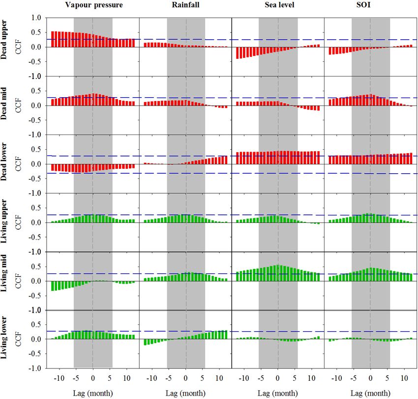
4710            J. Z. Sippo et al.: Reconstructing extreme climatic and geochemical conditions during mangrove dieback

Figure 1. Study sites of (a) the living mangrove area (green) and (b) the dead mangrove area (red) near the mouth of the Norman River,
Karumba, QLD. Note that the yellow crosses represent transects through the upper, middle and lower study sites. (c) The elevation above
the Australian Height Datum (AHD) from a lidar digital elevation model (DEM) was measured from the seaward mangrove edge in 2017,
from the same transects that samples were collected from in 2016, through the living (green line) and dead (red line) mangrove areas (data
available from http://wiki.auscover.net.au/wiki/Mangroves, last access: August 2019). The satellite images were sourced from © Google
Earth (2019) and the Queensland Government (2019).

did not change with different normalization approaches –               examine relationships between climate variables and Fe over
which they did not. This normalization reduces external ef-            a 2-year period, as records of all climate variables are in the
fects (Gregory et al., 2019) and allows a more direct com-             resolution of months, but the chronology of Fe (based on 14 C
parison between samples from living and dead forest areas.             dates) is in years.
Methods that provided absolute concentrations such as CRS
are simply referred to as concentrations. Growth rates (in
millimetres per year) were calculated as the measured in-              3     Results
crement divided by the difference in years (estimated from
14 C) between samples. De-trended growth rates were then
                                                                       3.1    Climatic conditions
calculated as the deviation from the exponential curve fitted
to growth rates for each sample. Water use efficiency (WUE)            The climate records over the last 3 decades reveal an un-
was calculated from 13 C isotope values (Van Der Sleen et              precedented combination of low sea levels and low annual
al., 2015). Differences in the WUE between living and dead             rainfall. The SOI is significantly correlated with all climate
mangrove areas were compared using a t test.                           variables (Pearson product moment correlation, P < 0.05).
   Cross correlations with a time lag of 1-month intervals             Lower sea levels and rainfall had previously occurred inde-
were used to evaluate the relationships between climatic vari-         pendently (Fig. 2). Since 1985, trends in the SOI index based
ables (the Southern Oscillation index, SOI; sea level; rainfall        on vapour pressure, precipitation and sea level observations
and vapour pressure) and wood density, elemental relative              show El Niño in 1983, 1987, 1992, 1994, 1998, 2015 and
concentrations and growth rates. SOI data and other climate            2016.
data were obtained from the Bureau of Meteorology (station
number 029028; 2019) and published reports (Jones et al.,              3.2    Wood samples and ages
2009; Harris et al. 2017). All climatic data were used with a
1-month resolution and were smoothed using a centred mov-              The ages of A. marina ranged from 15 ± 2 to 34 ± 2 years
ing mean. This time lag analysis was specifically chosen to            (Table 1). On average, the trees in the living and dead man-
                                                                       grove forests were 21 ± 4 and 34 ± 1 years old respectively.

Biogeosciences, 17, 4707–4726, 2020                                                        https://doi.org/10.5194/bg-17-4707-2020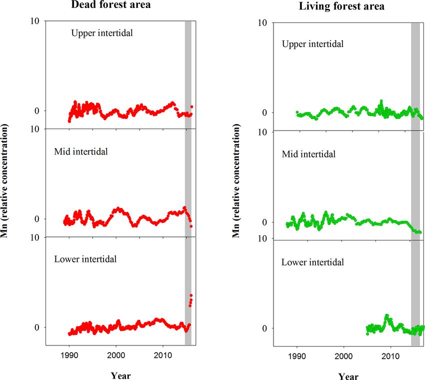
J. Z. Sippo et al.: Reconstructing extreme climatic and geochemical conditions during mangrove dieback 4711
the living mangrove area, peak wood Fe concentrations in the
upper, mid and lower intertidal areas were 25-, 4- and 3-fold
higher than their mean baseline concentrations respectively.
In the dead mangrove area, Fe levels were similar from the
upper to the lower intertidal zone (Fig. 3). In the living man-
grove area, Fe was highest in the upper and mid intertidal
zone and decreased in the lower intertidal zone. Itrax trends
are plotted against 14 C ages, and because tree growth rates
change over time, Itrax data are not evenly distributed over
time.
Significant correlations with no time lag were found be-
tween Fe in wood and vapour pressure, rainfall, sea level and
Southern Oscillation index (SOI; Fig. 4). All climate vari-
ables were strongly correlated with the SOI; therefore, we
could not separate the influence of individual climate vari-
ables on wood Fe. In the dead and living mangrove areas,
the strongest correlations with Fe occurred with no time lag
(Fig. 4).
Sediment cores had a similar pattern of decreasing Fe with
depth in the upper and lower intertidal areas as well as in liv-
ing and dead mangrove areas (Fig. 5a). Dead mangrove ar-
eas were depleted in Fe by ∼ 32 % in the surface 50 cm and
by ∼ 26 % in the surface 1 m relative to the respective living
mangrove areas in both the upper and lower intertidal areas
(Fig. 5b, c, d). Fe relative concentrations were significantly
higher in living mangrove areas compared with dead man-
grove areas (Mann–Whitney rank sum test, P < 0.001 for all
depths).
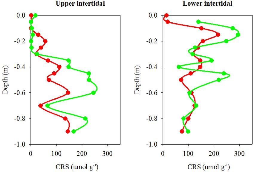
Chromium-reducible sulfur (CRS) absolute concentra-
tions, which provide a proxy for pyrite concentrations in sed-
iment cores, were also lower overall in the dead mangrove
area compared with the living mangrove area – by 36 %
in the upper and 38 % in the lower intertidal zones respec-
tively (Fig. 6). Although these differences were not signif-
icant (Mann–Whitney rank sum test, P > 0.05), they were
Figure 2. Climate observations from the south-eastern Gulf of Car- very similar to Itrax Fe trends. In the upper intertidal zone,
pentaria, Australian (Jones et al., 2009; Harris et al., 2017; Bureau CRS concentrations generally increased with depth, whereas
of Meteorology, 2019). The grey bar represents the period during
in the lower intertidal zone, CRS concentrations peaked from
which the dieback event occurred.
∼ 10 cm below the surface in both dead and living sediment
samples and then decreased with depth. Differences in CRS
Tree growth rates that were de-trended to negative exponen- concentrations (in both the upper and lower intertidal zones)
tial growth had no trends over time in either the living or dead between the dead and living mangroves were most prominent
mangrove areas (Table 1). in the upper ∼ 60 cm of each core and tended to converge at
greater depths (Fig. 6).
3.3 Fe in wood and sediment cores The water use efficiency (WUE) calculated from 13 C de-
creased in all wood samples from 1983 to 2017 (Fig. 7a),
Fe relative concentrations in all dead mangrove samples suggesting increasing water availability in the study area.
peaked at the time of mangrove mortality in late 2015–early During the dieback event, median WUE values were higher
2016 (Fig. 3). In the living mangrove samples, Fe peaked in in dead samples than in living samples, with the differ-
late 2015–early 2016 and then decreased in 2016 and 2017 ences being more pronounced in the upper intertidal zones
to long-term average levels. Peak wood Fe concentrations in (Fig. 7b). The comparison of the WUE in dead and living
the upper, mid and lower intertidal areas of the dead man- mangrove samples suggests lower water availability in the
grove samples were 40-, 90- and 30-fold higher respectively dead mangrove area (Fig. 7b). However, the mean WUE val-
than their mean baseline concentrations (i.e. the average Fe ues were compared from 1983 to 2017 and were not signifi-
concentrations in the sample prior to the dieback event). In cantly different (t test, P = 0.2) in dead and living mangrove
https://doi.org/10.5194/bg-17-4707-2020 Biogeosciences, 17, 4707–4726, 2020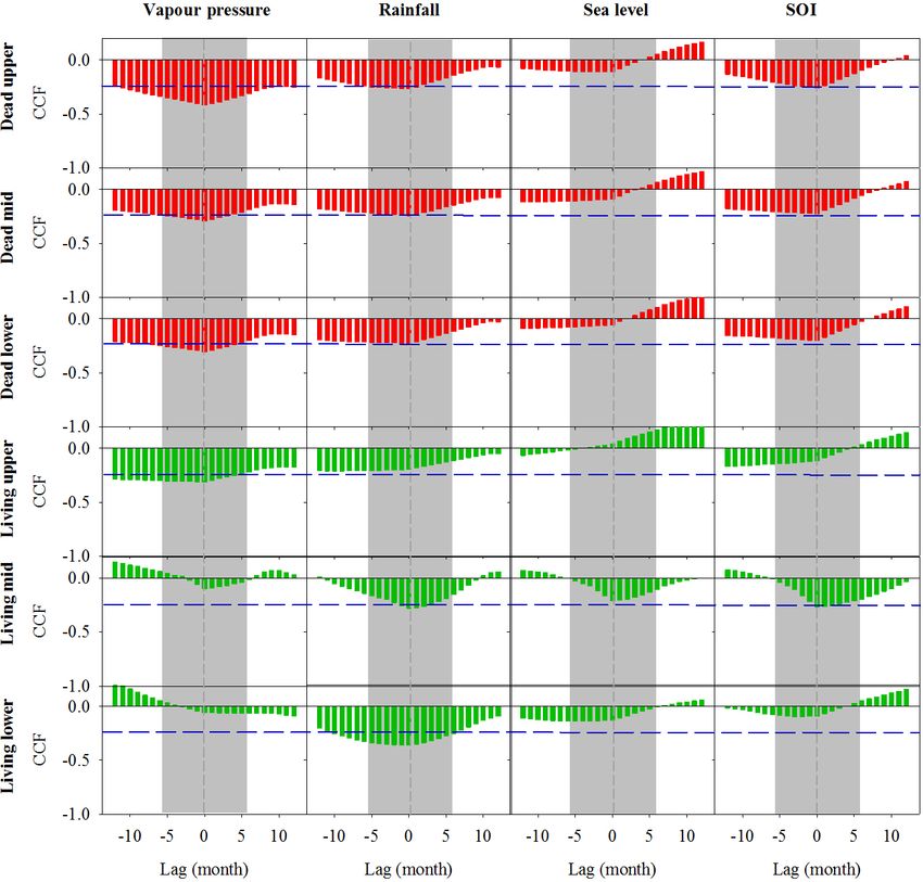
4712           J. Z. Sippo et al.: Reconstructing extreme climatic and geochemical conditions during mangrove dieback

Table 1. Summary of radiocarbon ages and growth rates (deviation from negative exponential growth) for all wood samples taken from dead
and living mangrove areas in the Gulf of Carpentaria, Australia.

                              Sample          Distance                14 C           Modelled           Deviation from
                                             from pith          mean ± 1σ         calendar age                 negative
                                                 (mm)             (pMC)a           mean ± 1σ         exponential growth
                                                                                     (year CE)              (mm yr−1 )
                                                                   Dead mangroves
                              Upper                   2     121.98 ± 0.28             1984 ± 2                             −
                              intertidal             17     119.82 ± 0.27             1986 ± 2                           −2.6
                                                     35     118.02 ± 0.27             1988 ± 2                           −1.4
                                                     52     116.07 ± 0.30             1990 ± 3                           −1.2
                                                     70     110.85 ± 0.26             1998 ± 2                           −4.7
                                                     87     105.35 ± 0.23             2010 ± 2                           −1.3
                                                     89                                 2015b                            −0.9
                              Mid                     2     123.56 ± 0.30             1983 ± 2                             −
                              intertidal             12     122.81 ± 0.30             1984 ± 2                            2.3
                                                     24     119.07 ± 0.28             1987 ± 2                           −4.8
                                                     36     115.92 ± 0.38             1991 ± 3                           −3.6
                                                     49     110.06 ± 0.27             1999 ± 2                           −3.7
                                                     62     105.17 ± 0.29             2011 ± 3                           −0.2
                                                     64                                 2015b                            −0.2
                              Lower                   2     123.31 ± 0.38             1983 ± 2                             −
                              intertidal             23     120.39 ± 0.36             1986 ± 2                           −2.3
                                                     45     117.35 ± 0.35             1989 ± 2                           −1.8
                                                     89     110.89 ± 0.33             1998 ± 2                           −1.9
                                                    110     105.75 ± 0.31             2009 ± 2                           −2.1
                                                    113                                 2015b                            −2.5
                                                                  Living mangroves
                              Upper                   2     163.84 ± 0.48             1995 ± 2                             −
                              intertidal             20     112.00 ± 0.42             1996 ± 3                            2.3
                                                     40     109.81 ± 0.44             2000 ± 3                           −0.8
                                                     58     103.71 ± 0.40             2013 ± 2                           −2.3
                                                     60                                 2017b                            −2.9
                              Mid                     2     113.32 ± 0.45             1994 ± 2                             −
                              intertidal             16     111.13 ± 0.31             1997 ± 2                           −1.0
                                                     33     109.22 ± 0.37             2001 ± 2                            0.8
                                                     49     106.59 ± 0.29             2014 ± 2                           −1.2
                                                     50                                 2017b                            −2.3
                              Mid                     2     113.41 ± 0.29             1993 ± 3                             −
                              intertidal             25     110.89 ± 0.28             1998 ± 2                           −1.0
                                                     50     101.91 ± 0.30             2017 ± 1                            0.2
                                                     51                                 2017b                            −2.3
                              Lower                   2     108.83 ± 0.27             2002 ± 2                             −
                              intertidal             17     107.30 ± 0.29             2005 ± 2                           −5.1
                                                     33     104.92 ± 0.37             2011 ± 3                            9.2
                                                     46     104.30 ± 0.34             2014 ± 2                           −2.3
                                                     48                                 2017b                            −2.2
                            a Measured 14 C content is shown in percent modern carbon (pMC; Stuiver and Polach, 1977).
                            b Year of collection of A. marina samples.

Biogeosciences, 17, 4707–4726, 2020                                                                      https://doi.org/10.5194/bg-17-4707-2020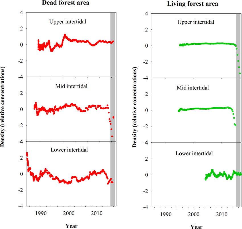
J. Z. Sippo et al.: Reconstructing extreme climatic and geochemical conditions during mangrove dieback                            4713

Figure 3. Fe relative concentrations in mangrove wood over time in living (green dots) and dead (red dots) mangroves from upper, mid and
lower intertidal areas in the Gulf of Carpentaria, Australia. Grey areas indicate the dieback event.

areas. Groundwater salinity values were highest in the upper          ples (comparative Fe loss) within the dead mangrove zone
intertidal mangrove areas and lowest in the lower intertidal          (Figs. 3, 5, 6) both suggest the mobilization of bioavailable
areas (Fig. 7c). Salinities were not significantly different in       Fe as Fe2+ . These observations are consistent with oscilla-
the living and dead forest areas (t test, P = 0.913).                 tions in sedimentary redox conditions, which are triggered
   Normalized wood density values in the dead mangrove                by changes in water availability, promoting the mobilization
forest showed no change during the dieback event in the up-           of Fe – firstly as bioauthigenic pyrite is oxidized and then
per intertidal zone, but a decline in density values occurred in      again during the reduction of Fe(III) oxide species when con-
the mid and lower intertidal zones (Fig. 8). In the living man-       ditions return to being predominantly anaerobic (Fig. 9). In-
grove area, declines in wood density values occurred in the           creased oxygen diffusion into sediments during the period
upper and mid intertidal zones during the mortality event, but        of low water availability likely resulted in the oxidation of
no variation in density occurred in the lower intertidal zone         bioauthigenic pyrite, which transformed into aqueous and
(Fig. 8).                                                             bioavailable Fe2+ (e.g. Fig. 9.2a; Johnston et al., 2011). With
                                                                      further oxidation, Fe2+ would likely have transformed into
                                                                      solid-phase Fe(III)oxides (Fig. 9.2b). Such Fe(III) oxides are
4     Discussion                                                      highly reactive; thus, any subsequent short-term reduction
                                                                      (e.g. due to tidal inundation) would also result in remobi-
4.1    Evidence of differences in water availability                  lization of Fe as Fe2+ (Fig. 9.2c). The fact that the trends
       between living and dead forest areas from                      in Fe that were observed in wood and soil samples were not
       dendrogeochemistry                                             observed for other elements analysed by Itrax supports the
                                                                      hypothesis that Fe trends were likely related to pyrite oxida-
Multiple lines of evidence from wood samples and sediment             tion and/or redox oscillations (Figs. A1, A2).
cores point to substantial differences in water availability be-         The most probable cause of a shift from reducing to ox-
tween the dead and living mangrove areas. For example, Fe             idizing conditions in the sediment is a reduction in water
trends in wood (comparative Fe gain) and sediment sam-

https://doi.org/10.5194/bg-17-4707-2020                                                       Biogeosciences, 17, 4707–4726, 2020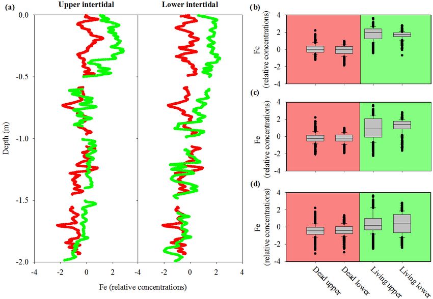
4714           J. Z. Sippo et al.: Reconstructing extreme climatic and geochemical conditions during mangrove dieback

Figure 4. Cross-correlation function (CCF) between Fe in wood samples and climate data at a 1-month resolution over a 12-month period
prior to and following dieback. Wood samples are from the upper, mid and lower intertidal zones of the dead (red) and living (green)
mangrove areas. Blue horizontal dashed lines indicate P < 0.01 with n = 125. Grey dashed vertical lines at zero lag indicate the dieback
period, and the grey bar represents the period during which the dieback event occurred.

content (Keene et al., 2014) associated with the intense El           similar trend: more enriched 13 C values in the dead mangrove
Niño of 2015–2016 and the related low sea levels and annual           zone.
rainfall (Fig. 2). Trends in wood density, mangrove growth
rate and water use efficiency also reveal distinct differences        4.2   Fe in wood
in water availability between dead and living forest areas.
Lower water availability in the dead mangrove forest area             The elemental composition of wood samples suggest that the
was also evident in the lower plant growth rates and higher           mangrove forest experienced sharp changes in sediment geo-
plant water use efficiency. Mangrove plant isotope data at the        chemistry during the dieback phase (Fig. 3). This is consis-
same sites from a study by Harada et al. (2020) also show a           tent with low sea levels and low rainfall (and likely ground-
                                                                      water) reducing soil water content, leading to the oxidation

Biogeosciences, 17, 4707–4726, 2020                                                       https://doi.org/10.5194/bg-17-4707-2020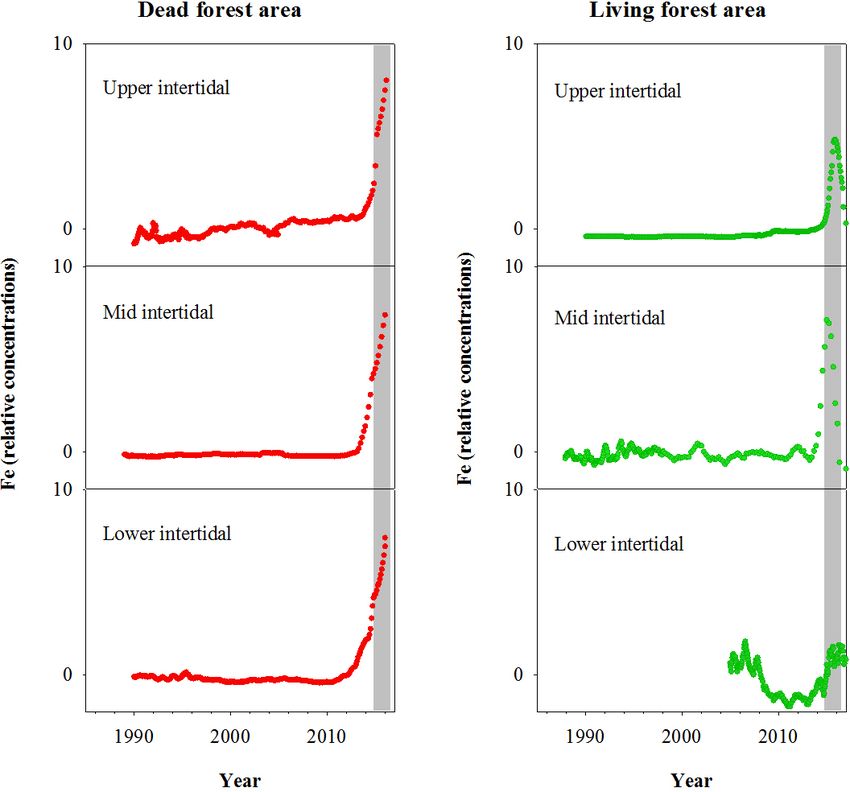
J. Z. Sippo et al.: Reconstructing extreme climatic and geochemical conditions during mangrove dieback                                4715

Figure 5. (a) Fe relative concentrations in sediment cores to 2 m depth from the upper and lower intertidal areas of living (green) and dead
(red) mangroves in the Gulf of Carpentaria, based on Itrax analysis. Box plots of normalized Fe relative concentrations from sediment cores
to depths of (b) 0.5 m, (c) 1 m and (d) 2 m. The central horizontal line represents the median value, the box represents the upper and lower
quartiles, and the whiskers represent the maximum and minimum values excluding outliers, i.e. the black dots.

Figure 6. Chromium reducible sulfur (CRS) profiles (a proxy for pyrite) from sediment cores in dead (red) and living (green) mangrove areas
in the Gulf of Carpentaria.

https://doi.org/10.5194/bg-17-4707-2020                                                          Biogeosciences, 17, 4707–4726, 2020
4716            J. Z. Sippo et al.: Reconstructing extreme climatic and geochemical conditions during mangrove dieback

Figure 7. (a) Changes in the water use efficiency (WUE) over time in wood samples collected from the upper, lower and mid intertidal zone
in living (green) and dead (red) mangrove areas. The grey bar represents the mangrove dieback event. Error bars are not visible due to the
low error of individual samples. (b) Box plot of the water use efficiency in mangrove wood samples in dead and living mangrove areas in
the upper, mid and lower intertidal zones. The sample size is greater than four from each wood sample. The central horizontal line represents
the median, the box represents the upper and lower quartiles, and the whiskers represent the maximum and minimum values. (c) Box plot
of groundwater salinity 8 months after the dieback event in the dead and living mangrove areas in the upper, mid and lower intertidal zones.
The sample size is greater than three from each intertidal zone.

of Fe sulfide minerals and the release of Fe2+ (Fig. 9.2a). The          living forest areas (Fig. 4). However, because all climate vari-
Fe peaks in the dead mangrove area at the time of tree mor-              ables were strongly correlated with each other, we could not
tality were 30- to 90-fold higher than baseline Fe (the mean             separate the relationships between individual climate drivers
Fe concentration in the sample prior to the dieback event).              and Fe trends. We speculate that the combination of the low
   In the living mangrove area, an Fe peak 25-fold higher                availability of fresh groundwater and low sea levels during
than baseline Fe was observed in the upper intertidal zone               the strong El Niño event of 2015–2016 are key drivers of the
(Fig. 3). In the mid and lower intertidal areas of the liv-              sediment redox conditions, as reflected in wood Fe trends.
ing mangroves, Fe peaks were 4- and 3-fold higher than                      Considering the extreme increases in Fe concentrations
baseline values respectively. In all living wood samples, Fe             observed in the wood samples during the dieback event, it
subsequently decreased after the dieback event, suggesting               is plausible that Fe toxicity could have contributed to man-
that Fe in new wood growth was diminished in associa-                    grove mortality. However, we cannot fully test this hypoth-
tion with a return to sustained reducing sediment conditions             esis in this study and are unaware of research testing the
and a concomitant attenuation in porewater Fe2+ availability             toxicity of Fe in A. marina at highly elevated concentrations
(Fig. 9.2d).                                                             of bioavailable Fe2+ . Alongi (2010) found that Fe toxicity
   Records of all climate variables are in the resolution of             occurred in some mangrove species at high concentrations
months, but the chronology of Fe (based on 14 C dates) is in             (100 mmol m2 d−1 of water-soluble Fe-EDTA) that were ap-
years. Therefore, we used time lag analysis to examine rela-             proximately 2-fold higher than the Fe supply for maximal
tionships between climate variables and Fe over a 2-year pe-             growth. However, A. marina (the dominant species affected
riod (Fig. 4). Fe wood concentrations were significantly cor-            by the dieback at the study site) appear relatively resilient to
related with both rainfall and vapour pressure in the dead and           high porewater Fe2+ . For example, Johnston et al. (2016) ob-

Biogeosciences, 17, 4707–4726, 2020                                                          https://doi.org/10.5194/bg-17-4707-2020
J. Z. Sippo et al.: Reconstructing extreme climatic and geochemical conditions during mangrove dieback                              4717

Figure 8. Normalized wood density (relative concentrations) in mangrove wood over time in living (green dots) and dead (red dots) mangrove
areas of the Gulf of Carpentaria, Australia. The grey bar represents the time period of the dieback event.

served no A. marina mortality at porewater Fe2+ concentra-             4.3   Fe in sediments
tions of 7- to 15-fold above normal in a mangrove forest im-
pacted by acid sulfate drainage. Considering that other man-           Sediment cores also displayed considerable differences in
grove species are affected by Fe toxicity at 2-fold the optimal        down-core Fe profiles between living and dead mangrove ar-
Fe availability, it is possible that a 30- to 90-fold increase in      eas (Fig. 5a, b). Normalized Fe concentrations were lower in
Fe could have been an additional stressor to mangroves al-             the upper 1 m of sediments in the dead mangrove area com-
ready stressed by low water availability.                              pared with the living, but they were very similar in sediments
   While our observations suggest that complex sedimentary             deeper than 1 m (Fig. 5a, b). Similar trends were also ob-
redox conditions occurred in dead-zone mangrove sediments              served in CRS (a proxy for pyrite, FeS2 ) sediment core pro-
during the dieback event, linking drought and low sea lev-             files, which have ∼ 40 % lower FeS2 concentrations in the
els to porewater Fe concentrations requires further investi-           dead mangroves in the upper 60 cm of the profile compared
gation. For example, crab burrows and root systems can in-             with the living mangrove sediments (Fig. 6). The fact that
duce conditions that increase O2 diffusion into sediments              differences in down-core trends in Fe are most prominent in
and, thus, influence Fe2+ mobility over tidal cycles (Nielsen          the upper parts of the sediment cores is consistent with de-
at al., 2003; Kristensen et al., 2008). Localized Fe(III) oxide        creases in water availability being more confined to the upper
dissolution can also occur in redox or pH micro-niches and             parts of the sediment profile, whereas deeper sediments are
under suboxic conditions (Fabricius et al., 2014; Zhu et al.,          more likely to have remained fully saturated.
2012). Further research on the mechanisms of bioavailable                 Although mangrove sediment conditions are typically
Fe release and the thresholds for Fe toxicities in A. marina           highly heterogeneous (Zhu et al., 2006; Zhu and Aller, 2012),
is required to clearly understand the impacts of porewater Fe          the sediment core results are broadly consistent with the
on mangrove forests.                                                   wood data. The apparent mobilization of Fe (loss from sed-
                                                                       iment and uptake in wood) was not observed in other ele-
                                                                       ments (Figs. A1, A2). Sediment Fe : Mn ratios in Itrax data

https://doi.org/10.5194/bg-17-4707-2020                                                         Biogeosciences, 17, 4707–4726, 2020
4718 J. Z. Sippo et al.: Reconstructing extreme climatic and geochemical conditions during mangrove dieback Figure 9. Conceptual diagram of Fe speciation under different sediment redox and pH conditions as well as (1) how speciation changes would be influenced by sea level and groundwater. Under initially elevated redox conditions due to low water availability (2) pyrite oxidation causes Fe transformation to (a) bioavailable Fe2+ and (b) particulate Fe(OH)3 followed by the eventual re-establishment of normal water availability and reducing conditions as well as (c) the consequent reduction of Fe(OH)3 and the generation of Fe2+ followed by (d) the sequestration of Fe(II) species via pyrite reformation. displayed no clear differences between living and dead man- similar to short-term porewater-derived dissolved Fe fluxes grove areas. These similarities may be because the sediment (79±75 mmol m2 d−1 ) estimated for a healthy temperate salt cores were taken after the dieback period when sediment marsh–mangrove system (Holloway et al., 2018) and provide geochemistry conditions returned to normal. Trends in Mn some comparative restraint for our estimates. in the wood samples (Fig. A1) also show no clear differences If our sediment cores in dead and living mangroves were between living and dead forest areas, and the Fe : Mn ratios representative of changes within the entire dieback area in the wood Itrax data overwhelmingly reflect the Fe concen- (7400 ha), then total Fe losses from the dieback event could trations. be equivalent to 87 ± 163 Gg Fe. This loss is equivalent to Sediment Fe losses, as implied by comparative Fe pro- 12 %–50 % of global annual Fe inputs to the surface ocean files (Figs. 3, 4, 6), also suggest a likely outwelling of Fe from aerosols (Jickells and Spokes, 2002; Fung et al., 2000; to the ocean. We estimate Fe outwelling by comparing FeS2 Elrod et al., 2004). As the surface ocean can be Fe limited, concentrations in living and dead mangrove sediment cores the consequences of Fe outwelling from a dieback event of based on the assumptions that (1) all Fe was originally in the this magnitude may have had an effect on productivity in the form of FeS2 and (2) tree Fe uptake is a minor loss path- Gulf of Carpentaria. way. The losses of Fe from the dead mangrove sediment would be equivalent to 87 ± 163 mmol m2 d−1 . The replica- tion of CRS sediment cores (n = 4) greatly limits the accu- racy of our estimates. However, these fluxes are remarkably Biogeosciences, 17, 4707–4726, 2020 https://doi.org/10.5194/bg-17-4707-2020
J. Z. Sippo et al.: Reconstructing extreme climatic and geochemical conditions during mangrove dieback                       4719

4.4   Wood density, growth trends and water use                     showed that no consistent differences in growth trends were
      efficiency                                                    identified between mangrove areas (Fig. 8). The lower in-
                                                                    tertidal sample of the living mangroves grew more quickly
Clear decreases in the normalized wood density were ob-             during the dieback, which may suggest optimal conditions
served during the mangrove mortality event (Fig. 8). Similar        during this time. This may be due to increased nutrient avail-
to trends in wood Fe, the wood density values in the living         ability stemming from litterfall inputs of organic matter from
and dead forest areas were correlated with climatic indica-         nearby stressed trees. All other sampled trees show no in-
tors (Fig. A3). In A. marina trees, the observed decreases          dication of reduced growth prior to or during the mortality
in wood density likely indicate decreased growth; however,          event (Table 1). We suggest that climatic conditions drove
the annual-scale resolution of 14 C ages prevented detection        very low growth rates during the dieback event, as indicated
of this short-term change in our growth rate data. Therefore,       by wood density data (Fig. 8) and previous studies that found
these clear decreases in wood density prior to tree mortal-         low growth during droughts (Cook et al., 1977; Santini et al.,
ity are an indication of stress, as decreased growth rates of       2013).
mangroves can be associated with decreased water availabil-            A significant difference in mean 13 C and WUE between
ity (Verheyden et al., 2005; Schmitz et al., 2006; Santini et       living and dead mangrove areas was observed in the upper
al., 2013), which is also directly related to increased salin-      intertidal zone (t test, P = 0.02), but not in the mid or lower
ity. Low rainfall conditions and increased temperatures in-         intertidal zones (Fig. 7b). This is consistent with the zona-
crease both evaporation and evapotranspiration while reduc-         tion of mangrove mortality which occurred predominantly
ing freshwater inputs (Medina and Francisco, 1997; Hoppe-           in the upper intertidal areas (Duke et al., 2017). The con-
Speer et al., 2013).                                                sistent decrease in the WUE suggests that water availability
   Interestingly, no decrease in density was observed in the        has been increasing over time in all intertidal areas since the
upper intertidal area of the dead mangroves (Fig. 8), despite       1990s (Fig. 7a). This is supported by generally increasing
the clear increase in Fe during the dieback in this tree sam-       precipitation since the 1980s (Fig. 2), which enhanced man-
ple (Fig. 3). This suggests that no change in growth occurred       grove areas in the Gulf of Carpentaria prior to this dieback
prior to tree mortality, implying rapid mortality in this case.     event (Asbridge et al., 2016). Therefore, climatic conditions
The upper intertidal area of the dead mangroves may have            were initially favourable over the plants lifetime, and trees
been living at the limit of its tolerance range with respect        may have been insufficiently acclimated to withstand drought
to water availability or salinity prior to the dieback, as sug-     and low soil water availability during the dieback. Overall,
gested by extremely high groundwater salinities in the upper        this highlights the important role of extreme climatic events
intertidal areas of dead and living mangrove forests 8 months       in counterbalancing mangrove responses to gradual climate
after the dieback event (Fig. 7c). No decrease in wood density      trends (Harris et al., 2018).
was observed in the lower intertidal area of the living man-
groves, which is consistent with both variation in the con-         4.5   Differences in water availability between living and
centration of Fe and tree growth rate data. Together, these               dead forest areas
data suggest that the lower intertidal area of the living man-
groves was not exposed to the same conditions during the            We have no data to determine if regional groundwater avail-
dieback event as areas in the dead mangroves higher in the          ability was greater in living forest areas than in dead forest
intertidal zone (Figs. 3, 8, 9). These results suggest a gradi-     areas during the mangrove dieback. No significant difference
ent of water availability, from extremely low availability at       was observed in groundwater salinities 8 months after the
the upper intertidal zone of the dead mangrove area to high         dieback. However, under normal sea level conditions (i.e.
or optimal availability at the lower intertidal zone of the liv-    when groundwater samples were collected), tidal inundation
ing mangrove area. As the elevation profiles are similar in         is likely to be the predominant driver of groundwater salin-
the dead and living mangrove areas in the lower and mid in-         ities rather than groundwater flows. Duke et al. (2017) and
tertidal areas (Fig. 1), it is possible that the difference in Fe   Harris et al. (2017) provide strong evidence that water avail-
trends between the mangrove areas is associated with the in-        ability in the Gulf of Carpentaria was extremely low prior to
fluence of regional groundwater flows on sedimentary redox          and during the dieback event. In this study, we have been able
conditions.                                                         to build on this work by exploring links between changes in
   Mean growth rates of trees in living (4.4 ± 3.6 mm yr−1 )        sediment geochemistry and low water availability.
and dead (5.3 ± 3.5 mm yr−1 ) mangrove areas are similar to            We eliminate elevation as a potential driver of water avail-
rates measured by Santini et al. (2013) in A. marina in arid        ability in living and dead forest areas. Tree mortality even
Western Australia (4.1–5.3 mm yr−1 ). However, there was            occurred in the lower intertidal zone of the dead mangrove
∼ 10-fold greater variability in the present study because          area which is at the same elevation as the lower intertidal
samples were collected from the upper, mid and lower in-            zone of the living forest area (see the elevation DEM in
tertidal zone, whereas Santini et al. (2012) sampled from           Fig. 1c). As other potential water sources were compara-
the lower intertidal zone only. De-trended growth rate data         ble between the sites, differences in water availability were

https://doi.org/10.5194/bg-17-4707-2020                                                    Biogeosciences, 17, 4707–4726, 2020
4720 J. Z. Sippo et al.: Reconstructing extreme climatic and geochemical conditions during mangrove dieback
likely driven by groundwater availability. Groundwater flows 5 Summary and conclusions
have high spatial variability and have been demonstrated to
be an important water source in mangroves from arid Aus- Wood and sediment geochemical data from living and dead
tralia. For example, Stieglitz (2005) highlights that the in- mangrove areas suggest that there were substantive differ-
terrelationships between confined and unconfined aquifers in ences in their comparative sediment redox conditions during
the coastal zone can result in localized differences in ground- the dieback event. Climatic data and patterns in Fe concen-
water flows. High-resolution spatial analysis of groundwater trations in wood and sediment samples suggest that sediment
salinities in living and dead forest areas during low sea level oxidation occurred in combination with unprecedented low
conditions would help to clarify how water sources may drive sea levels and low rainfall. As the elevation of dead and liv-
mangrove mortality. ing mangrove areas was very similar, we suggest that the dif-
ference in tree survival between areas was probably due to
4.6 Limitations higher groundwater availability at the living site. Evidence of
plant Fe uptake and losses of Fe from sediments are consis-
This study is inherently limited in its spatial extent. Thus, tent with this hypothesized Fe mobilization associated with
the differences in Fe between samples from living and dead low water availability in sediments. The dieback event was
mangrove areas may be due to causal factors beyond the likely a period of transitioning redox states in a heteroge-
scope of this study. However, the consistency of results from neous sediment matrix, which resulted in areas of mangrove
multiple methods and divergent sample types provides some sediments with low water availability combined with pore-
confidence in the interpretation that recent changes in sed- waters enriched in bioavailable Fe (Fig. 9).
iment geochemistry have occurred in association with ex- Our data suggest that extremely low water availability
treme drought and low sea level events. drove the mangrove dieback. However, mangrove dieback
Our analysis benefited from the development of high- may also be associated with increased concentrations of
precision 14 C dating of mangrove wood samples (with age bioavailable Fe2+ in porewaters that occurred during this
uncertainties of 1–3 calendar years, 1σ ; see Table 1) that rely time of low water availability. Estimated losses of Fe from
on the atmospheric bomb 14 C content resulting from above- sediments were consistent with the observed plant uptake and
ground nuclear testing mostly in the late 1950s and early suggest Fe mobilization due to sediment oxidation (and sub-
1960s (Hua and Barbetti, 2004). The complexity in the wood sequent reduction). This Fe mobilization may also have led
development of A. marina creates uncertainties (Robert et to significant Fe inputs to the ocean.
al., 2011). Secondary growth in A. marina is atypical, dis- This study supports climate observations suggesting that
playing consecutive bands of xylem and phloem which can the Gulf of Carpentaria dieback was strongly driven by an
result in multiple cambia (i.e. the tissue providing undiffer- extreme El Niño–Southern Oscillation (ENSO) event (Har-
entiated cells for the growth of plants) being simultaneously ris et al., 2017). Climate change is increasing the intensity
active (Schmitz et al., 2006; Robert et al., 2011). Further- of ENSO events and climate extremes (Lee and McPhaden,
more, A. marina cambia display non-cylindrical or asymmet- 2010; Cai et al., 2014; Freund et al., 2019) as well as in-
rical growth (Maxwell et al., 2018). These characteristics of creasing sea level variability (Widlansky et al., 2015), which
A. marina atypical growth can influence our results, as there is impacting on mangrove forests in arid coastlines (Love-
is variation within each stem. lock et al., 2017). Therefore, this study builds on the premise
As younger wood grows on the exterior of the tree, errors that the dieback event was associated with climate change
associated with the estimated ages do not introduce uncer- (Harris et al., 2018). Further research is necessary to under-
tainty in the direction of trends but decrease the ability to stand the role of Fe in tree mortalities, to constrain potential
find correlated trends with climatic variables (Van Der Sleen Fe losses to the ocean and from sediments, and to understand
et al., 2015). In spite of these uncertainties, the strong cross thresholds for Fe toxicities in A. marina.
correlations displayed in Fig. 4, with minimal time lag, sug-
gest that the dendrochronology results are robust and that cli-
mate variability drives long-term Fe cycling in the coastal
mangroves of the Gulf of Carpentaria.
Biogeosciences, 17, 4707–4726, 2020 https://doi.org/10.5194/bg-17-4707-2020J. Z. Sippo et al.: Reconstructing extreme climatic and geochemical conditions during mangrove dieback 4721 Appendix A Figure A1. Normalized Mn relative concentrations in mangrove wood over time in living (green dots) and dead (red dots) mangroves from upper, mid and lower intertidal areas of the Gulf of Carpentaria, Australia. Grey areas indicate the dieback event. https://doi.org/10.5194/bg-17-4707-2020 Biogeosciences, 17, 4707–4726, 2020
4722           J. Z. Sippo et al.: Reconstructing extreme climatic and geochemical conditions during mangrove dieback

Figure A2. Normalized Ca relative concentrations in mangrove wood over time in living (green dots) and dead (red dots) mangroves from
upper, mid and lower intertidal areas of the Gulf of Carpentaria, Australia. Grey areas indicate the dieback event.

Biogeosciences, 17, 4707–4726, 2020                                                     https://doi.org/10.5194/bg-17-4707-2020
J. Z. Sippo et al.: Reconstructing extreme climatic and geochemical conditions during mangrove dieback                            4723

Figure A3. Cross-correlation function (CCF) analysis of the relationship between wood density and climate data over time at a 1-month
resolution over a 12-month period prior to and following dieback. Wood samples are from the upper, mid and lower intertidal zones of the
dead (red) and living (green) mangrove areas. Blue horizontal dashed lines indicate P < 0.01 with n = 125. Grey dashed vertical lines at
zero lag indicate the dieback period.

https://doi.org/10.5194/bg-17-4707-2020                                                       Biogeosciences, 17, 4707–4726, 2020
4724            J. Z. Sippo et al.: Reconstructing extreme climatic and geochemical conditions during mangrove dieback

Data availability. Data will be made available online in the PAN-       Brookhouse, M.: Eucalypt dendrochronology: past, present and po-
GAEA data repository.                                                      tential, Aust. J. Bot., 54, 435–449, 2006.
                                                                        Burdige, D. J.: Estuarine and coastal sediments – coupled biogeo-
                                                                           chemical cycling, Treat. Estuar. Coast. Sci., 5, 279–316, 2011.
Author contributions. JZS and DTM conceived the research ques-          Bureau of Meteorology: Climate data online, available at: http://
tion, designed the study approach and led the field survey. IRS, CJS,      www.bom.gov.au/climate/data/, last access: 12 August 2019.
CL, NSS and SGJ helped interpret the data and aided with the de-        Burton, E. D., Bush, R. T., and Sullivan, L. A.: Sedimentary iron
sign of the paper. PG and QH provided specialized use of facilities        geochemistry in acidic waterways associated with coastal low-
and helped with the interpretation of data. YH and GR helped with          land acid sulfate soils, Geochim. Cosmochim. Acta, 70, 5455–
data collection. JZS wrote the first draft of the paper, and all co-       5468, https://doi.org/10.1016/j.gca.2006.08.016, 2006.
authors contributed to subsequent drafts of the paper.                  Burton, E. D., Sullivan, L. A., Bush, R. T., Johnston, S. G., and
                                                                           Keene, A. F.: A simple and inexpensive chromium-reducible sul-
                                                                           fur method for acid-sulfate soils, Appl. Geochem., 23, 2759–
Competing interests. The authors declare that they have no conflict        2766, 2008.
of interest.                                                            Cai, W., Borlace, S., Lengaigne, M., van Rensch, P., Collins,
                                                                           M., Vecchi, G., Timmermann, A., Santoso, A., McPhaden,
                                                                           M. J., Wu, L., England, M. H., Wang, G., Guilyardi E., and
                                                                           Jin, F. F.: Increasing frequency of extreme El Niño events
Acknowledgements. James Z. Sippo acknowledges funding sup-
                                                                           due to greenhouse warming, Nat. Clim. Change, 4, 111,
port and access to ANSTO facilities from AINSE which made this
                                                                           https://doi.org/10.1038/nclimate2100, 2014.
project possible. We would like to thank Jocelyn Turnbull for giv-
                                                                        Cook, E. R. and Jacoby, G. C.: Tree-ring-drought relationships in
ing us permission to use recent atmospheric 14 C data from Baring
                                                                           the Hudson Valley, New York, Science, 198, 399–401, 1977.
Head, Wellington. The study was funded by the Australian Research
                                                                        Donato, D. Kauffman, C., Murdiyarso, J. B., Kurnianto, D., Stid-
Council (grant nos. DE150100581, DP180101285, DE160100443,
                                                                           ham S. M., and Kanninen, M.: Mangroves among the most
DP150103286 and LE140100083).
                                                                           carbon-rich forests in the tropics, Nat. Geosci., 4, 293–297, 2011.
                                                                        Elrod, V. A., Berelson, W. M., Coale K. H., and Johnson, K. S.:
                                                                           The flux of iron from continental shelf sediments: A missing
Financial support. This research has been supported by the Aus-            source for global budgets, Geophys. Res. Lett., 31, L12307,
tralian Research Council (grant nos. DE150100581, DP180101285,             https://doi.org/10.1029/2004gl020216, 2004.
DP150103286, DE160100443 and LE140100083).                              Fabricius, A.-L., Duester, L., Ecker, D., and Ternes, T. A.: New Mi-
                                                                           croprofiling and Micro Sampling System for Water Saturated En-
                                                                           vironmental Boundary Layers, Environ. Sci. Technol., 48, 8053–
Review statement. This paper was edited by Ji-Hyung Park and re-           8061, 2014.
viewed by two anonymous referees.                                       Farquhar, G., K. Hubick, Condon, A., and Richards, R.: Carbon iso-
                                                                           tope fractionation and plant water-use efficiency, Stable isotopes
                                                                           in ecological research, Springer, New York, 21–40, 1989.
                                                                        Farquhar, G. and Richards, R.: Isotopic composition of plant carbon
References                                                                 correlates with water-use efficiency of wheat genotypes, Funct.
                                                                           Plant Biol., 11, 539–552, 1984.
Alber, M., Swenson, E. M., Adamowicz, S. C., and Mendelssohn,           Fink, D., Hotchkis, M., Hua, Q., Jacobsen, G., Smith, A. M., Zoppi,
  I. A.: Salt Marsh Dieback: An overview of recent                         U., Child, D., Mifsud, C., van der Gaast, H., and Williams, A.:
  events in the US, Estuar. Coast. Shelf Sci., 80, 1–11,                   The antares AMS facility at ANSTO, Nucl. Instrum. Methods
  https://doi.org/10.1016/j.ecss.2008.08.009, 2008.                        Phys. Res. B, 223, 109–115, 2004.
Alongi, D. M.: The Impact of Climate Change on Man-                     Freund, M. B., Henley, B. J., Karoly, D. J., McGregor, H. V., Abram,
  grove Forests, Curr. Clim. Change Rep., 1, 30–39,                        N. J., and Dommenget, D.: Higher frequency of Central Pacific
  https://doi.org/10.1007/s40641-015-0002-x, 2015.                         El Niño events in recent decades relative to past centuries, Nat.
Asbridge, E., Lucas, R., Ticehurst, C., and Bunting, P.: Mangrove          Geosci., 12, 450–455, https://doi.org/10.1038/s41561-019-0353-
  response to environmental change in Australia’s Gulf of Carpen-          3, 2019.
  taria, Ecol. Evol., 6, 3523–3539, 2016.                               Fung, I. Y., Meyn, S. K., Tegen, I., Doney, S. C., John, J. G., and
Asbridge, E., Bartolo, R., Finlayson, C. M., Lucas, R. M.,                 Bishop, J. K.: Iron supply and demand in the upper ocean, Global
  Rogers, K., and Woodroffe, C. D.: Assessing the distribution             Biogeochem. Cy., 14, 281–295, 2000.
  and drivers of mangrove dieback in Kakadu National Park,              Gilman, E. L., Ellison, J., Duke, N. C., and Field, C.: Threats to
  northern Australia, Estuar. Coast. Shelf Sci., 228, 106353,              mangroves from climate change and adaptation options: A re-
  https://doi.org/10.1016/j.ecss.2019.106353, 2019.                        view, Aquat. Bot., 89, 237–250, 2008.
Barbier, E. B., Hacker, S. D., Kennedy, C., Koch, E. W.,                Google Earth: Karumba, Qld, Australia, Digital Globe, 2019.
  Stier, A. C., and Silliman, B. R.: The value of estuarine             Gregory, B. R. B., Patterson, R. T., Reinhardt, E. G., Galloway, J.
  and coastal ecosystem services, Ecol. Monogr., 81, 169–193,              M., and Roe, H. M.: An evaluation of methodologies for calibrat-
  https://doi.org/10.1890/10-1510.1, 2011.                                 ing Itrax X-ray fluorescence counts with ICP-MS concentration
Bronk Ramsey, C.: Deposition models for chronological records,
  Quat. Sci. Rev., 27, 42–60, 2008.

Biogeosciences, 17, 4707–4726, 2020                                                         https://doi.org/10.5194/bg-17-4707-2020
You can also read