Reconstructing the 2015 Salgar flash flood using radar retrievals and a conceptual modeling framework in an ungauged basin - Hydrol-earth-syst-sci.net
←
→
Page content transcription
If your browser does not render page correctly, please read the page content below
Hydrol. Earth Syst. Sci., 24, 1367–1392, 2020
https://doi.org/10.5194/hess-24-1367-2020
© Author(s) 2020. This work is distributed under
the Creative Commons Attribution 4.0 License.

Reconstructing the 2015 Salgar flash flood using radar retrievals
and a conceptual modeling framework in an ungauged basin
Nicolás Velásquez1,2,3 , Carlos D. Hoyos1,2 , Jaime I. Vélez1 , and Esneider Zapata2
1 Universidad Nacional de Colombia, Sede Medellín, Facultad de Minas, Departamento de Geociencias y Medio Ambiente,
Medellin, Colombia
2 Sistema de Alerta Temprana de Medellín y el Valle de Aburrá (SIATA), Área Metropolitana del Valle de Aburrá (AMVA),

Medellin, Colombia
3 Iowa Flood Center, University of Iowa, C. Maxwell Stanley Hydraulics Laboratory 135, Iowa City, Iowa, USA

Correspondence: Nicolás Velásquez (nvelasqg@unal.edu.co)

Received: 25 August 2018 – Discussion started: 25 September 2018
Revised: 12 December 2019 – Accepted: 24 January 2020 – Published: 24 March 2020

Abstract. On 18 May 2015, a severe rainfall event triggered       ening the entire basin before the occurrence of the flash flood
a flash flood in the municipality of Salgar, located in the       event and impacting the subsurface–runoff partitioning dur-
northwestern Colombian Andes. This work aims to recon-            ing the flash flood event. Evidence suggests that the spatial
struct the main hydrological features of the flash flood to       structure of the rainfall is at least as important as the geomor-
better understand the processes modulating the occurrence of      phological features of the basin in regulating the occurrence
the event. Radar quantitative precipitation estimates (QPEs),     of flash flood events.
satellite information, and post-event field visits are used to
reconstruct the Salgar flash flood, in an ungauged basin,
addressing the relationship among rainfall spatiotemporal
structure, soil moisture, and runoff generation during succes-    1   Introduction
sive rainfall events by using a conceptual modeling frame-
work including landslide and hydraulic submodels. The hy-         Flash floods are regarded as one of the most destructive hy-
drological model includes virtual tracers to explore the role     drological hazards, resulting in considerable loss of human
of runoff and subsurface flow and the relative importance of      life and high costs due to infrastructure damage (Roux et al.,
convective and stratiform precipitation in flash flood gen-       2011; Gruntfest and Handmer, 2001). Among all different
eration. Despite potential shortcomings due to the lack of        types of floods, Jonkman (2005) shows that flash floods re-
data, the modeling results allow an assessment of the im-         sult in the highest average mortality rate per event (3.62 %),
pact of the interactions between runoff, subsurface flow, and     almost 10 times larger than the mortality rate for river floods.
convective–stratiform rainfall on the short-term hydrologi-       Flash floods are usually described as rapidly rising water-
cal mechanisms leading to the flash flood event. The over-        level events occurring in steep streams and rivers, associ-
all methodology reproduces the magnitude and timing of the        ated with short-term, very intense convective precipitation
La Liboriana flash flood peak discharge considerably well,        systems or orographically forced rainfall events over highly
as well as the areas of landslide occurrence and flood spots,     saturated land surfaces and steep terrains (Šálek et al., 2006;
with limitations due to the spatial resolution of the avail-      Llasat et al., 2016; Douinot et al., 2016). Convective precip-
able digital elevation model. Simulation results indicate that    itation episodes often feature high intensity, short duration,
the flash flood and regional landslide features were strongly     and relatively reduced spatial coverage (Houze, 2004).
influenced by the antecedent rainfall, which was associated          Several authors have assessed the role of the geologi-
with a northeasterly stratiform event. The latter recharged the   cal and geomorphological features of the catchment, soil
gravitational and capillary storages within the model, moist-     type, soil moisture conditions, and spatiotemporal structure
                                                                  of rainfall in flash flood occurrence, identifying the lead-

Published by Copernicus Publications on behalf of the European Geosciences Union.
1368                                                  N. Velásquez et al.: Reconstructing the 2015 flash flood event of Salgar

ing causative mechanisms of this hazard (Merz and Blöschl,            The topography of Colombia is characterized by three
2003). Adamovic et al. (2016) and Vannier et al. (2016) re-        branches of the Andes crossing the country south-to-north,
lated the flash floods governing processes to the geological       generating a mixture of landscapes from high snow-capped
properties of the basins, with mixed results. Wu and Sidle         mountains, vast highland plateaus, and deep canyons to wide
(1995) emphasized the role of the topography, ground cover,        valleys, making some regions highly prone to flash flood oc-
and groundwater in the occurrence of shallow landslides and        currence. The likelihood of flash flood occurrence in Colom-
associated debris flows. Many authors have assessed the in-        bia is also high due to the spatiotemporal behavior of the In-
fluence of hills and stream slopes, suggesting the slopes of       tertropical Convergence Zone and the direction of the near-
the hills are significantly more important for flash flood oc-     surface moist air flow leading to orographic enhancement of
currence and magnitude than the slope of the stream (Šálek         convective cores (Poveda et al., 2007). In the last decade,
et al., 2006; Roux et al., 2011; Yatheendradas et al., 2008;       there have been several widespread and localized flash flood
Younis et al., 2008). Rodriguez-Blanco et al. (2012) ana-          events in Colombia associated with climatological features
lyzed flash flood episodes in Spain and determined that an-        and the local intensification of rainfall events. According to
tecedent soil moisture conditions play a significant role in       estimates by the Comisión Económica para América Latina
runoff production. Castillo et al. (2003) also suggested a sig-    y el Caribe, the 2010–2011 La Niña event alone triggered
nificant correlation between flash flood magnitude and the         1233 flooding events and 778 mass removal processes in
antecedent moisture conditions. Aronica et al. (2012) used         Colombia, with more than 3 million people affected and
spatial and statistical analysis to reconstruct landslides and     damages estimated at more than USD 6.5 billion.
deposits, finding a connection between flash flood occur-             Since the 2010 widespread disaster, several isolated events
rence and soil moisture antecedent conditions.                     have occurred in the country, with devastating consequences.
   The fact that small basins are more prone to flash floods       The present paper focuses on studying the processes trigger-
(Wagener et al., 2007) makes their measurement difficult           ing a flash flood in La Liboriana basin, a 56 km2 basin lo-
and, consequently, their understanding and their prediction        cated in the western range of the Colombian Andes, as a re-
(Hardy et al., 2016; Ruiz-Villanueva et al., 2013; Yamanaka        sult of consecutive rainfall storms that took place between
and Ma, 2017; Borga et al., 2011; Marra et al., 2017). The         15 and 18 May 2015. The resulting flash flood dramatically
local rainfall storm events related to flash floods require that   affected the region, causing more than 100 casualties, affect-
high spatiotemporal resolution be characterized (Norbiato          ing several buildings and critical infrastructure, and resulting
et al., 2008). Some authors follow a climatological approx-        in a total reconstruction cost estimated at COP 36 000 mil-
imation to assess the recurrence of flash floods in particular     lion (about USD 12.5 million considering the 2018 exchange
regions, focusing on the atmospheric causative mechanisms.         rate), which corresponds to 3 times the annual income of the
For example, Kahana et al. (2002) examined the extent to           municipality. Figure 1 shows an example of infrastructure
which floods in the Negev Desert are the outcome of clima-         damage and changes in the basin’s main channel as a result of
tological synoptic-scale features, finding that about 80 % of      the flash flood event, showing considerable river margin and
the events can be linked to distinct synoptic conditions oc-       bed erosion. Despite the data scarcity, including of discharge
curring days prior to the flood events. Schumacher and John-       measurements, the analysis of the successive rainfall events
son (2005) studied extreme rain events associated with flash       triggering the Salgar flash flood provides an interesting case
flooding in the United States over a 3-year period, using the      study for assessing the mechanisms that depend on the soil
national radar reflectivity composite data. They found that        moisture conditions and rainfall distribution.
65 % of the total number of flash floods are associated with          La Liboriana is a typical case of an ungauged basin
mesoscale convective systems (MCSs), with two recurrent            (Sivapalan et al., 2003; Seibert and Beven, 2009; Beven,
patterns of organization: the existence of training convective     2007; Bonell et al., 2006; Yamanaka and Ma, 2017), with-
elements and the generation of quasi-stationary areas of con-      out any detailed records of soils or land use, topographic
vection with stratiform rainfall downstream. Fragoso et al.        maps or high-resolution digital elevation models (DEMs),
(2012) analyzed storm characteristics and rainfall conditions      and scarce hydro-meteorological data. According to Blöschl
for flash flood occurrence at Madeira (Portugal), and their        et al. (2012), there are three general strategies for using mod-
results suggest an essential role of global climate patterns       els under these conditions. The first strategy is to obtain
(North Atlantic Oscillation – NAO – forcing) and local forc-       the required model parameters from the historical basin be-
ing (orographic features) in the triggering of such events.        havior and the morphological characteristics of the basin.
Implicitly, these studies and all the others available in the      This strategy often leads to low model performance (Duan
peer-reviewed literature point to the need for local and re-       et al., 2006). The second approach is to inherit the hydrolog-
gional high-quality spatiotemporal rainfall data. Berne and        ical model calibration from a neighboring gauged watershed,
Krajewski (2013) highlighted the need to incorporate high-         which in this case does not exist. The third method is to pa-
resolution weather radar information, even with some limita-       rameterize the model based on proxy variables, such as hy-
tions, in flash flood hydrology.                                   draulic information obtained during field visits. In the case of
                                                                   the 2015 La Liboriana basin flash flood, there are no previous

Hydrol. Earth Syst. Sci., 24, 1367–1392, 2020                                    www.hydrol-earth-syst-sci.net/24/1367/2020/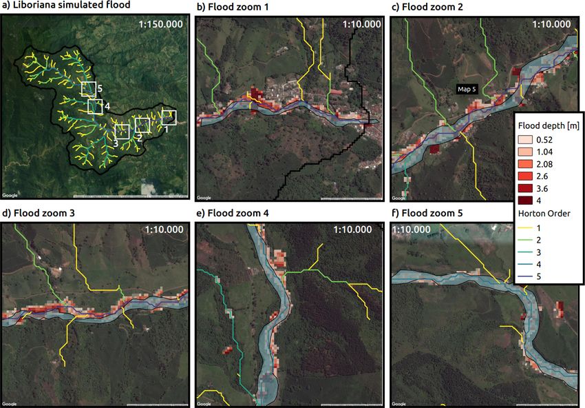
N. Velásquez et al.: Reconstructing the 2015 flash flood event of Salgar                                                        1369

                                                                     scheme, including landslide and hydraulic submodels, to as-
                                                                     sess the potential occurrence of flash flood events.
                                                                        We use the WMF (Watershed Modeling Framework),
                                                                     which includes a variation of the TETIS hydrological model
                                                                     (Vélez, 2001; Francés et al., 2007), modified to include
                                                                     a shallow landslide submodel, and a floodplain submodel
                                                                     called HydroFlash. The TETIS model is a cell-distributed
                                                                     conceptual hydrological model that uses storage tanks and
                                                                     the kinematic wave approximation to simulate the most rele-
                                                                     vant processes in the basin. The landslide submodel is a sta-
                                                                     bility model that classifies cells into unconditionally stable,
                                                                     unconditionally unstable, and conditionally stable depend-
                                                                     ing on geomorphology; conditionally stable cells are further
                                                                     classified as stable or unstable based in their variable water
                                                                     content (Aristizábal et al., 2016). HydroFlash is a low-cost
                                                                     1-D model that estimates the cross-sectional filled area at all
                                                                     time steps on the basis of the liquid discharge and the sedi-
                                                                     ment transport. In addition, the TETIS model was modified
                                                                     to include four virtual tracers to separately explore the role of
                                                                     runoff and subsurface flow as well as the relative importance
                                                                     of convective and stratiform precipitation in flash flood gen-
                                                                     eration. The assessment of the interactions between runoff,
                                                                     subsurface flow, and convective–stratiform rainfall allows a
                                                                     better understanding of the short-term hydrological mecha-
                                                                     nisms leading to the flash flood event.
                                                                        The document is structured as follows. Section 2 describes
                                                                     in more detail the region of study, La Liboriana basin, in-
                                                                     cluding geomorphological and climatological characteristics
                                                                     of the basin and the information sources used in this assess-
                                                                     ment. Section 3 presents a description of the overall method-
Figure 1. Example of infrastructure damage as a result of the La     ology and the TETIS model, including flow separation, and
Liboriana flash flood event on 18 May 2015. (a) Aerial photo-        the shallow landslide and HydroFlash submodels. Section 4
graph taken before the event (2012), during a mission of the De-     describes the main results of the study, including model vali-
partment of Antioquia’s government, and (b) a satellite image af-    dation and sensitivity analysis, and presents results from the
ter the event (courtesy of CNES/Airbus via © Google Earth). The      landslide and HydroFlash submodels. Section 5 includes a
images show the destruction of most houses in that particular com-   discussion on the role of the rainfall structure in the flash
munity, a bridge over La Liboriana, and the main road. All of the
                                                                     flood reconstruction. Finally, the conclusions are presented
houses shown in the 2015 image had to be either demolished or
structurally repaired. The images also show changes in the delin-
                                                                     in Sect. 6.
eation of the main channel as well as considerable erosion in the
river margins.
                                                                     2     Study site and data

                                                                     2.1    Catchment description

historical streamflow records nor records from a neighboring         The urban area of the municipality of Salgar is located near
watershed; thus, we followed the third approach. We use pre-         the outlet of La Liboriana basin, a small (56 km2 ) tropical
cipitation information derived from radar, satellite and aerial      watershed located in the westernmost range of Colombia’s
images, in addition to post-event field visits, to reconstruct       Andes (Fig. 2). By 2015, Salgar counted 17 400 inhabitants,
the Salgar flash flood event. This study addresses two broad         including 8800 residing in the urban area. La Liboriana basin
hydrological issues. The first issue consists in exploring the       joins the El Barroso river basin, and both drain to the Cauca
relationship between rainfall spatiotemporal structure (Llasat       River.
et al., 2016; Fragoso et al., 2012), soil moisture and runoff           The availability of the ALOS-PALSAR DEM (ASF,
generation (Penna et al., 2011; Tramblay et al., 2012; Garam-        2011), with a resolution of 12.7 m, allows us to estimate
bois et al., 2013) during the successive rainfall events and the     the main geomorphological features of the basin. The av-
second one in proposing a simplified hydrological modeling           erage slope of La Liboriana is 57.6 %, and the basin longi-

www.hydrol-earth-syst-sci.net/24/1367/2020/                                        Hydrol. Earth Syst. Sci., 24, 1367–1392, 2020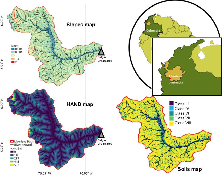
1370                                                   N. Velásquez et al.: Reconstructing the 2015 flash flood event of Salgar

Figure 2. Geographical context of the Liboriana basin, located in Colombia, in the Department of Antioquia. The panels include the map of
slopes, the height above the nearest drainage (HAND), and the soil type map. The HAND values were estimated using a 12.7 m resolution
digital elevation model (DEM). Low HAND values correspond to areas prone to flooding. Note that the soil type map is an extrapolation of
the soil properties as a function of slope.

tude and perimeter are 13.5 and 57.8 km, respectively. The             are values close to 0 m. High HAND values in the upper re-
Strahler–Horton order of the main stream is 5, and its lon-            gion of the watershed often denote areas of high potential en-
gitude and slope are 18.1 km and 8.1 %, respectively. The              ergy, with increased sediment production and frequent shal-
highest elevation of the watershed (Cerro Plateado) reaches            low landslide occurrence. Banks with low HAND values are
3609 m a.s.l. (above sea level), while the outlet of the basin is      more susceptible to flooding and tend to correspond to ar-
at 1316 m a.s.l. The 99th slope percentile of order 1 streams          eas prone to extensive damages caused by extreme events.
is 78 %. For streams of order 2 to 5, the 99th slope percentiles       The social challenges lie in the high vulnerability of Salgar,
are 61 %, 27 %, 18 % and 11%, respectively. Figure 2 shows             given the location of the main urban settlement.
the spatial distribution of the slopes in the watershed. These            Vegetation and land use vary considerably within the
features are typical of Andean mountainous basins. Geomor-             basin. Figure 3 shows land use in different regions of the wa-
phologically, this kind of watershed tends to be prone to the          tershed from a 2012 aerial image. In the upper region of the
occurrence of flash floods (Lehmann and Or, 2012; Penna                La Liboriana basin, there is dense vegetation (see Zoom 1 in
et al., 2011; Martín-Vide and Llasat, 2018; Longoni et al.,            Fig. 3), with a high percentage of the area covered by tropical
2016; Ozturk et al., 2018; Khosravi et al., 2018; Marchi et al.,       forests and presence of grass and few crop fields. A portion of
2016; Bisht et al., 2018).                                             the upper watershed is considered a national park. Hillslopes
   At the subbasin scale, La Liboriana exhibits a vast range           near the divide do not show significant anthropic interven-
of slopes and altitude differences. Figure 2 shows the height          tion, most likely due to the steepness of this region. Down the
above the nearest drainage (HAND) model (Rennó et al.,                 hills and at the bottom of the valley, there are coffee planta-
2008) for La Liboriana. The HAND calculates the relative               tions (the primary economic activity of the region) and pas-
height difference between cell i and its nearest streamflow            tures. Downstream (Fig. 3, Zoom 2), the presence of crops
cell j . La Liboriana HAND exhibits values between 500 and             is evident among forest and grass areas. Near the middle of
800 m. Near the outlet of the basin, over the banks, there             the basin (Fig. 3, Zoom 3), the presence of crops is more ob-

Hydrol. Earth Syst. Sci., 24, 1367–1392, 2020                                        www.hydrol-earth-syst-sci.net/24/1367/2020/
N. Velásquez et al.: Reconstructing the 2015 flash flood event of Salgar                                                                  1371

Figure 3. Aerial overview of La Liboriana basin (source: © Department of Antioquia). The top-right panel presents the entire basin, showing
the locations of key regions detailed in the following panels, in zooms 1 to 5. The stream network is also presented, colored by order, from
yellow to deep blue corresponding to orders 1 to 5.

vious, and human settlements and roads start to appear. The             Table 1. Description of the soils in the region (Osorio, 2008).
watershed exhibits grazing areas and urban development near
the river banks. In Fig. 3, the Zoom 4 corresponds to the first           Type         Slope   Depth   Retention   Permeability   Percentage
                                                                                                (m)
affected urban area from upstream to downstream during the
flash flood. It is also possible to see a marked presence of              Class III     < 12    0.6    Low         High                  3.2
crops and some patches of forest. Finally, Zoom 5 shows the               Class IV     12–25    0.6    Mean        Mean                  8.3
                                                                          Class VI     25–30    1.0    Mean        Mean                  2.1
main urban area of Salgar surrounded by crops, grass and an               Class VII    30–50    0.3    Too low     Low                  25.5
important loss of forest coverage.                                        Class VIII    > 50    0.2    Too low     Low                  60.0
   One of the challenges for hydrological modeling and risk
management in the country is that soils are not well mapped;
the national soil cartography is usually available at a 1 :
400 000 scale. At this scale, the municipality of Salgar, in-           basin. During the campaign, we measured sectional distances
cluding La Liboriana basin, corresponds to only one category            and the surface water speed, at different points of the stream-
of soil texture. Osorio (2008), based on field campaign obser-          flow. The surface water speed was measured using a hand-
vations and laboratory tests, described La Liboriana soils as           held Stalker Pro II velocity radar. We also identified tradi-
well drained with poor retention capacity. Organic material             tional post-event terrain, land cover, vegetation and infras-
is predominant in the first layer, and clay loam soil predom-           tructure markers to record the approximate level associated
inates within the second layer. The depth of the soil is hill-          with the peak flow during the flash flood. Figure 4 presents
slope dependent, varying from 20 cm to 1 m (Osorio, 2008).              the selected cross section used for the estimation of the max-
Table 1 provides a summary of soil characteristics for five             imum discharge during the flash flood given its geometrical
different categories, all as a function of slope. Each soil cate-       and hydraulic regularity. The section has a rectangular shape,
gory has a corresponding depth and a qualitative description            a width of 4.6 m and a height of 5 m for a total area of 23 m2 .
of permeability and retention.                                          A visual inspection of the flooded house around the section,
                                                                        located 4–5 m away from the channel, reveals the presence of
2.2   Flash flood post-event observations                               mud marks on the walls with heights varying between 0.5 and
                                                                        1.2 m (see Fig. 4). The area of the section plus the flooded
We conducted a field campaign a few days after the 18 May               area during the event was estimated to be 37 m2 . During the
flash flood to assess the cross-sectional geometry along the            campaign, the surface speeds in the channel varied between
main channel in different sites, including at the outlet of the         2 and 3 m s−1 , for a 3 m3 s−1 discharge. Instrumented basins

www.hydrol-earth-syst-sci.net/24/1367/2020/                                            Hydrol. Earth Syst. Sci., 24, 1367–1392, 2020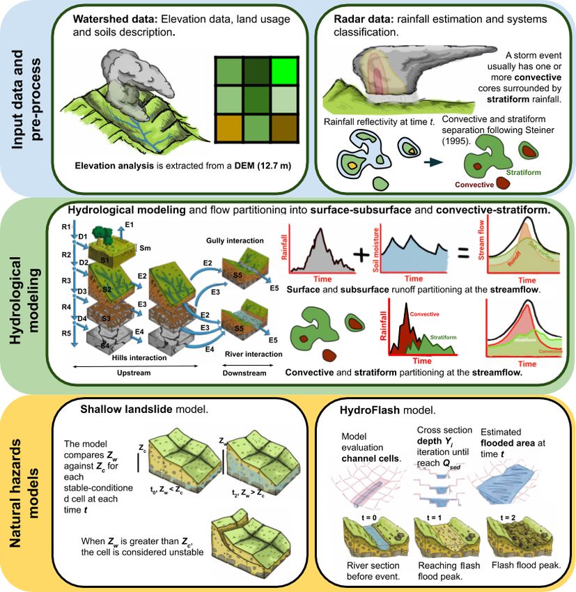
1372                                                   N. Velásquez et al.: Reconstructing the 2015 flash flood event of Salgar

                                                                     Hoyos (2017), using radar reflectivity fields, rainfall gauges
                                                                     and disdrometers. The QPE technique uses retrievals from a
                                                                     C-band polarimetric Doppler weather radar operated by the
                                                                     Sistema de Alerta Temprana de Medellín y el Valle de Aburra
                                                                     (SIATA, a local early warning system from a neighboring re-
                                                                     gion, https://siata.gov.co/siata_nuevo, last access: 25 Febru-
                                                                     ary 2020). The radar is 65 km away from the basin. It has
                                                                     an optimal range in a radius of 120 km for rainfall estima-
                                                                     tion and a maximum operational range of 240 km for weather
                                                                     detection. The radar operating strategy allows precipitation
                                                                     information to be obtained at a 5 min time step, with a spa-
                                                                     tial resolution of about 128 m. Despite the distance between
Figure 4. Channel cross section showing an example of flooded in-    the radar and the basin, and the mountains between them,
frastructure during the flash flood event. The section shows mud     there are no blind spots for the radar. A comparison between
marks on the walls of adjacent houses, with heights varying be-      the radar QPE estimates and records from two rain gauges
tween 0.5 and 1.2 m. The houses in the picture are located 4–5 m     installed 3 d after the flash flood event show a correlation
away from the channel. The photograph also shows the width of the    for an hourly timescale of 0.65. A detailed description of
channel and the total estimated depth during the flash flood. The    the rainfall estimation, as well as the overall meteorologi-
cross section is downstream from the bridge shown in the picture.
                                                                     cal conditions that led to the La Liboriana extreme event, are
                                                                     described in a companion paper (Hoyos et al., 2019). Radar
in the region, with similar characteristics in terms of area and     retrievals are also used to classify precipitation into convec-
slopes, show peak flow surface water speeds ranging between          tive and stratiform areas following a methodology proposed
5 and 7 m s−1 (see Fig. A1). By assuming an area of 37 m2            by Yuter and Houze (1997) and Steiner et al. (1995), based
and velocities between 5 and 6, we estimate that the flash           on the intensity and sharpness of the reflectivity peaks. The
flood peak flow was between 185 and 222 m3 s−1 . Local au-           methodology has been widely used in tropical regions as re-
thorities reported that the peak streamflow reached the urban        ported in the review by Houze et al. (2015).
perimeter after 02:10 LT on 18 May (personal communica-                  Between 15 and 18 May 2015, several storms took place
tion during the field visit). Reports state that the peak flow in    over La Liboriana basin. During the night of 17 May, be-
the most affected community occurred near 02:40 LT1                  tween 02:00 and 09:00 LT (local time), a precipitation event
   Aerial information before and after the occurrence of the         covered almost all of the basin (hereafter referred to as pre-
event is relevant to analyze the locations of the landslides         cipitation Event 1). Twenty hours later, between 23:00 LT
and flooded areas. During 2012, the Department of Antio-             on 17 May and 02:00 LT on 18 May, two successive ex-
quia conducted a detailed aerial survey of the municipality          treme convective systems occurred over the basin with the
of Salgar, and a few days after the event, DigitalGlobe and          maximum intensity in the upper hills (precipitation Event 2).
CNES/Airbus made available highly detailed satellite im-             Event 1 corresponds mainly to a stratiform event with an av-
ages of the same region. We performed a detailed contrast            erage precipitation accumulation of 47 mm over the basin.
between both products by using a geographic information              Event 2 corresponds to a moderate average of 38 mm; how-
system (QGIS), which provided us with information about              ever, the accumulation exceeded 180 mm over the upper wa-
flooded areas and landslide locations (see Figs. 1 and 16).          tershed. Hoyos et al. (2019) show that the individual events
Field campaign peak flow estimates and aerial imagery are            during May 2015 were not exceptional, the climatological
used to validate the results obtained with the TESTIS model.         precipitation anomalies were negative to normal, and the syn-
                                                                     optic patterns associated with the extreme events were sim-
2.3    Rainfall information                                          ilar to the expected ones for the region. However, the com-
                                                                     bination of high rainfall accumulation in a 96 h period as a
The assessment of the 2015 Salgar flash flood event follow-          result of successive precipitation events over the basin, fol-
ing a hydrological modeling strategy uses a radar-based QPE          lowed by a moderate extreme event during 18 May, is unique
technique described in Sepúlveda (2016) and Sepúlveda and            in the available observational radar record, in particular for
   1 As                                                              the upper part of the basin. Figure 5a presents the temporal
           reported by the media and the national
                                                                     evolution of the estimated convective–stratiform rainfall par-
government:               http://www.elcolombiano.com/antioquia/
tragedia-en-antioquia-salgar-un-ano-despues-XX4145514        (last
                                                                     titioning during both Events 1 and 2. The main difference
access: 15 May 2016), https://caracol.com.co/emisora/2015/12/        between both events is the timing of the convective versus
25/medellin/1451076926_792470.html (last access: 25 Decem-           stratiform participation within each case. Event 1 started as
ber 2015), http://portal.gestiondelriesgo.gov.co/Paginas/Noticias/   a stratiform precipitation event moving northeastward, from
2015/Antecion-Emergencia-Salgar-Antioquia.aspx (last access:         the Department of Chocó to the Department of Antioquia
19 May 2015).                                                        across the westernmost Andes mountain range. After 3 h

Hydrol. Earth Syst. Sci., 24, 1367–1392, 2020                                     www.hydrol-earth-syst-sci.net/24/1367/2020/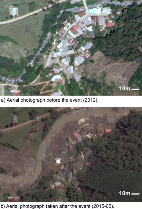
N. Velásquez et al.: Reconstructing the 2015 flash flood event of Salgar                                                                1373

Figure 5. (a) Temporal evolution of the convective–stratiform rainfall partitioning during both Events 1 and 2 (precipitation intensity in
mm h−1 , for 5 min periods). The figure shows the total rainfall (yellow) and the convective (blue) and stratiform (green) portions integrated
over La Liboriana basin. (b, c) Spatial distribution of the cumulative rainfall during Events 1 and 2 over La Liboriana basin, respectively.

of stratiform rainfall, training convective cores move over              3     Methodology
La Liboriana basin, generating intense precipitation peaks
in a 2.5 h period. It is important to note that these cores              3.1    TETIS hydrological model
did not strengthen within La Liboriana basin; these systems
formed and intensified over the western hills of Farallones              We used a physically based, distributed hydrological model
de Citará, draining to the Department of Chocó towards the               developed and fully described in Vélez (2001) and Francés
Atrato River. This is not a minor fact because, as a result              et al. (2007). The spatial distribution and the hydrological
of the latter process, the maximum intensity cores did not               flow path schema are based on the 12.75 m resolution DEM.
fall over the steepest hills of La Liboriana basin, but rather           In each cell, five tanks represent the hydrological processes,
near the basin outlet where the slopes are considerably flat-            including capillary (tank 1), gravitational (tank 2), runoff
ter. Figure 5b shows the spatial distribution of cumulative              (tank 3), baseflow (tank 4) and channel storage tanks (tank 5).
rainfall during Event 1, with the maximum precipitation lo-              The state of each tank varies as a function of vertical and
cated toward the bottom third of the basin. Event 2, on the              lateral flows as shown in Fig. 6, where the storage is rep-
other hand, started as a thunderstorm training event with two            resented by Si (mm) and the vertical input to each tank by
convective cores moving from the southeast, followed by the              Di (mm), which in turns depends on the vertical flow through
remaining stratiform precipitation. Even though the average              tanks Ri (mm). Ei (mm) represents the downstream connec-
cumulative rainfall over the basin was 9 mm less than during             tion between cells, except for tank 1, where E1 represents the
Event 1, this event is characterized by orographic intensifica-          evaporation rate.
tion within the basin, leading to a more heterogeneous spatial              The original model is modified to improve the representa-
distribution with the highest cumulative precipitation in the            tion of the flow processes that occur during flash floods (see
steepest portion of the basin (see Fig. 5b).                             Sect. 3.1.1). In addition, two analysis tools of the TETIS re-
   The data requirements and rainfall preprocessing needed               sults are introduced: virtual tracers tracking convective and
for the overall methodology followed in the reconstruction               stratiform precipitation as well as water paths over or through
of the 2015 Salgar flash flood are summarized in Table 2 and             the soils and a catchment-state analysis by cell grouping (see
are presented in a schematic diagram in Fig. 6.                          Fig. 13). The goal is to analyze the spatially distributed re-
                                                                         sponse of the watershed to precipitation events of a distinct
                                                                         nature.

www.hydrol-earth-syst-sci.net/24/1367/2020/                                             Hydrol. Earth Syst. Sci., 24, 1367–1392, 2020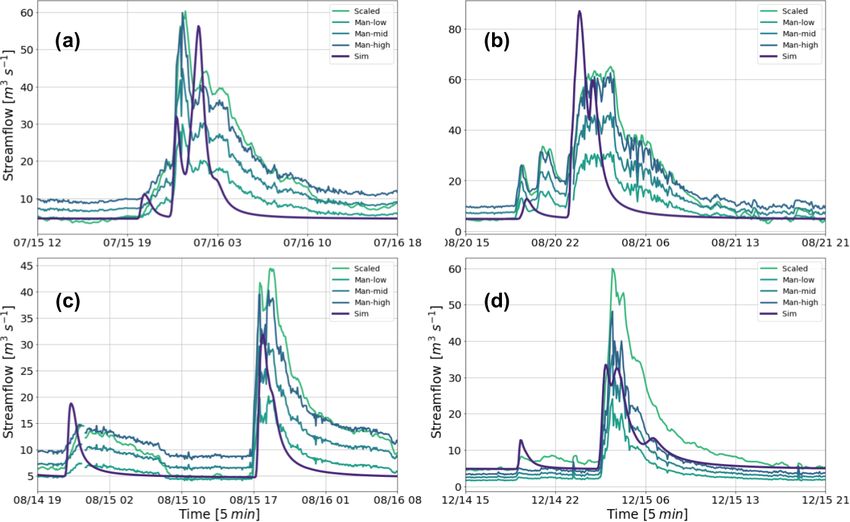
1374                                                      N. Velásquez et al.: Reconstructing the 2015 flash flood event of Salgar

Figure 6. Illustrative diagram of the methodology followed in the present study. The top row represents the key input data, specifically
a DEM and radar-based QPE as the basis of the modeling framework. The second row represents the conceptual basis of the TETIS model.
In each cell, five tanks represent the hydrological processes, including capillary (tank 1), gravitational (tank 2), runoff (tank 3), baseflow
(tank 4) and channel storage (tank 5). The state of each tank varies as a function of vertical and lateral flows as shown in the diagram, where
the storage is represented by Si and the vertical input by Di , which in turns depends on the vertical flow through tanks Ri . Ei represents
the downstream connection between cells and evaporation. The implementation of convective and stratiform rainfall separation and virtual
tracers is also portrayed. The implementations of the landslide and HydroFlash submodels are schematized in the bottom row.

3.1.1   Lateral flow modeling modifications                               follows:

The TETIS model relies on the concept of mass balance                     Ai (t) = Si (t)Fc /L,                                            (2)
where the storage of tank i at the end of the simulation in-              where L depends on the model √       cell width 1x (m), L =
terval Si (t)∗ (mm) is a function of the storage at the start of          1x for orthogonal flow and L = 21x for diagonal flow,
the simulation interval Si (t) (mm) and the storage outflow               and Fc (m3 mm−1 ) is a unit conversion factor that is equal
Ei (t) (mm) during the interval t, as follows:                            to the area of each cell element Ae (m2 ) multiplied by
                                                                          1 m/1000 mm. According to Vélez (2001), Ei changes as a
Si (t)∗ = Si (t) − Ei (t).                                       (1)      function of Ai , the flow speed vi (m s−1 ), and the model time
                                                                          step 1t (s), as follows:
The storage outflow Ei is estimated by transforming the stor-
age Si (t) into an equivalent cross-sectional area Ai (m2 ), as           Ei (t) = Ai (t)∗ vi (t)1t/Fc .                                   (3)

Hydrol. Earth Syst. Sci., 24, 1367–1392, 2020                                            www.hydrol-earth-syst-sci.net/24/1367/2020/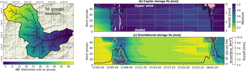
N. Velásquez et al.: Reconstructing the 2015 flash flood event of Salgar                                                              1375

Table 2. Summary of the data used for the setup of TETIS.

            Item                Description/source                    Period                  Usage
            Radar data          QPE rainfall estimations              17 to 18 May 2015       TETIS runs, rainfall characterization
                                                                                              and event analysis.
            Field campaign      Maximum streamflow estimation         20 May 2015             TETIS model comparison for
                                through visual inspection                                     indirect validation.
            Satellite imagery   Visible channel compositions          May 2015                Flash flood model validation,
                                from the DigitalGlobe CNES            (post-event)            shallow landslide model
                                imagery                                                       validation, and comparison
                                                                                              with pre-event conditions.
            Aerial photos       Aerial photos taken by the            2012                    Pre-event condition
                                government of Antioquia                                       comparison.
                                during 2012
            Soil description    Physical description of the soils     2008                    Simulations using TETIS
                                of the region by Osorio (2008)                                (model setup).

The expression for the cross-sectional area at the end of                The nonlinear Eq. (7) corresponds to an adaptation of
the simulation period Ai (t)∗ is found by replacing Si (t)               the Kubota and Sivapalan (1995) formula for subsurface
in Eq. (2) for Si (t)∗ and then the resulting expression and             runoff vi,4 , where ki,s is the saturated hydraulic conductiv-
Eq. (3) into Eq. (1):                                                    ity of cell i and the exponent b is dependent on the soil type,
                                                                         and it is assumed to be equal to 2. Ai,g is the equivalent cross-
              Si (t)Fc                                                   sectional area of the maximum gravitational storage (Hi,g –
Ai (t)∗ =                .                                      (4)
            L + vi (t)1t                                                 mm). Ai,3 is the corresponding sectional area for the gravita-
                                                                         tional storage (Si,3 ) obtained by using Eq. (4). There is also
Equation (4) is solved coupled with the equation for the
                                                                         return flow from tank 3 to tank 2, when Si,3 = Hi,g , which
speed vi :
                                                                         represents runoff generation by saturation. In the case of the
vi (t) = βAi (t)α .                                             (5)      baseflow, we assume that the speed vi,4 is constant for each
                                                                         cell and depends on the aquifer hydraulic conductivity ki,p
Equation (5) is the generic formulation for the speed used in            (see Eq. 8).
this work to represent nonlinearities in the relationship be-                                 2
tween vi and Ai . In the formulation, both β and α change,                              ki,s Mi,0
                                                                         vi,3 = C8                    Ai,3 (t)b                           (7)
depending on the type of flow: overland, subsurface, base,                             (b + 1)Abi,g
and channel flow. The solution for vi is obtained by using the
                                                                         vi,4 = C9 ki,p                                                   (8)
successive substitution method described by Chapra (2012).
In the model, we use a 5 min time step, which ensures the sta-           Finally, the streamflow velocity is calculated by using the
bility of the computations. When a solution is reached, Ei is            geomorphological kinematic wave approximation (Vélez,
computed using Eq. (3) and Si is updated using Eq. (1).                  2001; Francés et al., 2007), in which 3 (km2 ) represents the
   Nonlinear equations in lateral flows result in a better rep-          upstream area, and  and ωi , a regional coefficient and re-
resentation of processes at high resolutions (Beven, 1981;               gional exponents, respectively:
Kirkby and Chorley, 1967). A nonlinear approximation of
                                                                                      ω1 ω2            ω
runoff is presented in Eq. (6). This approximation is a modi-            vi,5 = C10 Mi,0 3i Ai,53 .                                      (9)
fication of Manning’s formula for flow in gullies. According
to Foster et al. (1984), ε and e1 are a coefficient and an ex-           An extended discussion of the regional parameters can be
ponent used to translate the Manning channel concept into                found in Vélez (2001). The streamflow speed expression is
                                                                                                                                   ω1
multiple small channels or gullies. The values of ε and e1               a version of Eq. (5), this considering that the terms , Mi,0 ,
                                                                           ω
                                                                         3 2 , and the exponent ω3 are constant with time.
are 0.5 and 0.64, respectively (Foster et al., 1984). Ai,2 (m2 )
is the corresponding sectional area obtained from Si,2 by us-            3.1.2       Tools for spatial analysis of the results: virtual
ing Eq. (4). In addition, Mi,0 is the slope of the cell, and ni is                   tracers and catchment cell grouping
the Manning coefficient.
         ε 1/2                                                           Virtual tracers are implemented in the model to discriminate
vi,2 = C7 Mi,0 Ai,2 (t)(2/3)e1                                  (6)      the streamflow sources into surface runoff and subsurface
         n

www.hydrol-earth-syst-sci.net/24/1367/2020/                                               Hydrol. Earth Syst. Sci., 24, 1367–1392, 2020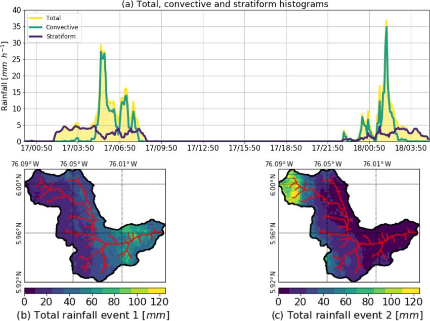
1376                                                  N. Velásquez et al.: Reconstructing the 2015 flash flood event of Salgar

flow and to assess the portion of streamflow from convective        prior to Event 1. Before this period, there were only a couple
rainfall and stratiform precipitation, recording the source at      of weak rainfall events; for this reason, the overall wetness
each time step and for each cell. The model archives the re-        was set to represent dry conditions at the start of the simu-
sults of the virtual tracing algorithm at the outlet of the basin   lation. Table 3 shows the mean value for all of the parame-
and for each reach, enabling us to study the different flow         ters used in the model and the scalar factor adjusted during
paths and water origins at different spatial scales.                the model calibration phase. For the 2015 Salgar flash flood
   The flow-tracing module operates in tanks 2 (runoff stor-        reconstruction, we calibrate the evaporation rate, the infiltra-
age) and 3 (subsurface storage). The module marks wa-               tion, the percolation, the overland flow speed, and the subter-
ter once it reaches either of these tanks, and the runoff–          ranean flow speed (see Table 3). The values for uncalibrated
subsurface flow percentage is taken into account once the           parameters are inherited from a local watershed with similar
water enters tank 5 (the channel). At this point, the scheme        characteristics.
assumes that the water in the channel is well mixed, implying
that the flow percentage is constant until new water enters the     3.2   Landslide submodel
channel.
   With a similar concept, the model also follows convec-           The landslide submodel coupled to the TETIS model is pro-
tive and stratiform rainfall. For this, at each time step, the      posed by Aristizábal et al. (2016). The stability of each cell
model takes into account the rainfall classified as convective      is calculated through the assessment of the different stresses
or stratiform and assumes that at each particular cell, the pre-    applied to the soil matrix. The coupling between TETIS and
cipitation is either entirely convective or entirely stratiform.    the landslide submodel is required because the stability of the
This assumption could lead to estimation errors at basins rep-      soil decreases with the porewater pressure (Graham, 1984).
resented by coarse cells (low DEM resolution) where convec-         The saturated soil depth Zi,w depends on the gravitational
tive and stratiform precipitation are likely to coexist. In the     storage Si,3 (t), the soil wilting point Wi,pwp , and the soil field
present study, the spatial resolution of the DEM is 12.7 m,         capacity Wi,fc , as follows:
higher than the resolution of the radar retrievals, so the po-                       Si,3 (t)
tential convective and stratiform rainfall concurrence is very      Zi,w (t) =                   .                                        (10)
                                                                                 Wi,cfc − Wi,pmp
low, and it could not be identified using the Steiner et al.
(1995) approach.                                                    When Zi,w is greater than the critical depth Zi,c (Eq. 11),
   Additionally, we propose a graphical method to analyze,          failure occurs. The critical saturated depth depends on the
at the same time, the evolution of multiple hydrological vari-      shallow soil depth Zi , the soil bulk density γi , the water den-
ables in the entire basin. The first step is to classify all the    sity γw , the gradient of the slope Mi,0 , the soil stability an-
cells within the watershed in a predetermined number of             gle φi , and the soil cohesion Ci0 .
groups according to their localization and the distance to the               γi

                                                                                          tan Mi,0

                                                                                                                 Ci0
outlet. The aim is to establish a coherent and robust spatial       Zi,c =      Zi 1 −               +         2
                                                                                                                                 (11)
discretization, thus allowing the concurrent spatiotemporal                  γw            tan φi        γw cos Mi,0 tan φi
variability of the different processes to be summarized in 2-       Figure 7 describes the variables of the model and the balance
D diagrams.                                                         of forces considered, and Table 4 presents the required pa-
                                                                    rameters for this model. According to the soil stability defini-
3.1.3   TETIS model calibration                                     tion, the topography and the soil properties, all cells are clas-
                                                                    sified into three classes: unconditionally stable, conditionally
The TETIS model requires a total of 10 parameters. Table 3          stable and unconditionally unstable. In particular, three pa-
includes all the parameters used in the model. The values           rameters determine the stability of each cell: (i) residual soil
of the parameters were derived from the soil properties de-         water table Zi,min (Eq. 12), (ii) the maximum soil depth at
scribed in Sect. 2. Due to the lack of detailed information in      which a particular soil remains stable Zi,max (Eq. 13), and
the region, parameters such as the infiltration and percolation     (iii) the maximum slope at which the soil remains stable Mi,c
rates are assumed to be constant in the entire basin. Other         (Eq. 14).
parameters, such as the capillary and gravitational storages,
                                                                                                        Ci0
vary as a function of the geomorphological characteristics          Zi,min =                                                             (12)
of the basin such as the elevation and slope. The calibration                  γw cos2 Mi,0 tan φi + γi cos2 Mi,c tan Mi,0 − tan φi
consists of finding the optimal scaling for each physical pa-                                   Ci0
                                                                    Zi,max =                                                             (13)
rameter, using a constant value for the entire basin (Francés                γi cos2 Mi,0 tan Mi,c − tan φi
et al., 2007). The model simulation is set to reach a base flow
                                                                                               γw

of 3 m3 s−1 , a value that corresponds to the discharge mea-        Mi,c = tan−1 tan φi 1 −                                               (14)
                                                                                               γi
surements during field campaigns days and weeks after the
flash flood event, during dry spells. To set the soil wetness       A cell is unconditionally stable when Zi is smaller
initial conditions realistically, the model simulations start 2 d   than Zi,min or when the cell slope is smaller than Mi,0 . On

Hydrol. Earth Syst. Sci., 24, 1367–1392, 2020                                       www.hydrol-earth-syst-sci.net/24/1367/2020/
N. Velásquez et al.: Reconstructing the 2015 flash flood event of Salgar 1377
Table 3. TETIS model parameters. Primed variables correspond to values prior to calibration. Values for the parameters with a scalar factor
of 1 are left uncalibrated. Parameters C1 to C6 are not presented in the explanation of the model. C1 modulates the maximum capillary
storage and C2 the maximum gravitational storage. C3 to C5 modulate evaporation, infiltration, and percolation rates, respectively. C6 is
assumed to be zero, as this variable determines the subterranean system losses. More detail about the calibration parameters is presented in
Francés et al. (2007).
Parameter name Symbol Scalar factor Spatial distribution
Capillarity storage H u = H u0 C1 (mm) C1 = 1 As a function of the slope
Gravitational storage Hg = H g 0 C2 (mm) C2 = 1 As a function of the slope
Evaporation rate Etr = Etr0 C3 (mm s−1 ) C3 = 0.1 As a function of the DEM
Infiltration rate ks = ks0 C4 (mm s−1 ) C4 = 2.7 Lumped
Percolation rate kp = kp0 C5 (mm s−1 ) C5 = 0.8 Lumped
System losses kf = kf0 C6 (mm s−1 ) C6 = 0.0 Lumped
Surface speed v2 = v20 C7 (m s−1 ) C7 = 0.5 Coefficient β of Eq. (6)
Subsurface speed v3 = v30 C8 (m s−1 ) C8 = 1 Coefficient β of Eq. (7)
Subterranean speed v40 = v40 C9 (m s−1 ) C9 = 0.5 Lumped
Channel speed v5 = v50 C10 (m s−1 ) C10 = 1 Coefficient β of Eq. (9)
including sediment load (Qi,load ), a realistic channel width is
calculated according to the Leopold (1953) approach as
Wi = 3.26Q−0.469
i , (15)
where Qi corresponds to the streamflow estimated based on
a long-term water balance.
Assuming an infinite sediment and ruble supply, Eqs. (16–
(18) are used to deduce, from the channel width Wi , the wa-
ter level Yi (Eq. 16), the friction velocity vi,fr (Eq. 16, de-
scribed in Takahashi, 1991), the sediment concentration ci
(Eq. 18), and finally the sediment-loaded stream discharge
(Eq. 20), as follows:
Figure 7. Schematic diagram of the landslide submodel. The figure Qi,sim (t)
and description are adapted from Aristizábal et al. (2016). QL and Yi (t) = , (16)
vi,sim (t)Wi
QR are the resultant forces on the sides of the slice of soil.
vi,sim (t)
vi,fr (t) = , (17)
Yi (t)
5.75 log D i,50
+ 6.25
the other hand, a cell is unconditionally unstable when Zi is 0.2
greater than Zi,max , and finally, a cell is conditionally stable ci (t) = Cmax (0.06Yi (t)) vi,fr (t) , (18)
when Zi is between Zi,min and Zi,max . Shallow landslides
1/2
are calculated at each time step of the hydrological simula-
1 g γw
tion, based on the latter cell class, where the soil stability de- ri (t) = ci + (1 − ci )
Di,50 0.0128 γsed
pends on the storm event, becoming unstable when Zi,w (t) is " 1/3 #
greater than Zi,c . Cmax
· −1 , (19)
ci
3.3 Floodplain submodel (HydroFlash) Qi,sim (t)
Qiload (t) = , (20)
1 − ci (t)
The HydroFlash submodel is designed to interpret the TETIS
simulations as floodplain inundations (Fig. 8). For each where vi,sim and Qi,sim are the simulated velocity and
stream cell and at each time step, the submodel (i) calcu- streamflow, respectively. Also, ri is the constitutive coeffi-
lates the stream discharge including sediment load (Eqs. 15– cient of the flow, which summarizes the flow dynamics as-
20; see Takahashi, 1991) and (ii) determines the inundated sociated with sediments and colliding particles. The above-
cells according to the stream cross profile, the sectional area, mentioned relationships depend on two parameters: the max-
and the stream velocities when including the sediment load imum sediment concentration (Cmax (–)) and the character-
(Eqs. 19–21, Takahashi, 1991). To determine the discharge istic diameter of the sediments Di,50 (m). Both terms are
www.hydrol-earth-syst-sci.net/24/1367/2020/ Hydrol. Earth Syst. Sci., 24, 1367–1392, 20201378 N. Velásquez et al.: Reconstructing the 2015 flash flood event of Salgar
Table 4. Landslide model parameters.
Parameter name Symbol Scalar Mean Spatial distribution
parameter value
Soil depth Zi (mm) 3.5 300 As a function of the slope
Topography slope Mi,0 (–) 1 0.01–5.3 From the DEM
Soil bulk density γsed (KN m−3 ) 1 18 Assumed constant
Water density γw (KN m−3 ) 1 9.8 Constant
Soil stability angle φi (◦ ) 1 30◦ Assumed constant
Soil cohesion Ci0 (KN) 1 4 Assumed constant
Figure 8. Illustrative diagram of the HydroFlash submodel scheme. Step 1: the submodel extracts the cross profile from the network con-
sidering the DEM and flow direction. Step 2: based on Eq. (21), the submodel obtains the first approximation of the flash flood streamflow;
then, the flood depth and the cross-sectional area are obtained from Eqs. (22) to (21). Step 3: the submodel obtains the flooded portion of the
cross section. Step 4: erosion post-process. Step 5: filling post-process. Step 6: the final result for a time step t.
assumed to be constant and equal to 0.75 (Obrien, 1988) rection changes from orthogonal to diagonal across or vice
and 0.138 (Golden and Springer, 2006), respectively. versa. We included two post-processing steps to correct these
To determine the inundated cells, the flood depth (Fi,d ) and issues by (i) using an image processing erosion algorithm
the sectional area of the stream including sediments (Ai,load ) (Serra, 1983) to remove the small and isolated flood spots
are iteratively calculated by reducing the difference be- (step 4 in Fig. 8) and, to solve the flow direction discontinu-
tween Qi,load and Q̂i,load . The channel cross section for ities, (ii) for each flooded cell the model seeks to inundate the
cell i, Ei,bed , is defined by the DEM. In each iteration N , the eight neighboring cells: a neighboring cell is also flooded if
model updates Fi,d with a 1y = 0.1 m increase. The cross- the altitude of the original flooded cell, plus the flood depth,
sectional area Ai,load is calculated by taking the difference is higher than its elevation (step 5 in Fig. 8). The image ero-
between Fi,d and the elevation of each cell j in the cross sec- sion is performed once with a 3-by-3 kernel. An example of
tion Ei,bed . the final result for a time step t is shown in step 6 in Fig. 8.
3
Q̂i,load (t) = 0.2ri (t)(N 1y) 2 Si,0 Ai,load (t) (21)
N
Fd,i N−1
= Fd,i + 1y (22) 4 Results
N
X The main results of the present study include the reconstruc-
AN
i,load = 1x
N
Fi,j,d N
− Ei,j,bed with Ei,j,bed < Fi,j,d (23) tion of the 2015 Salgar flash flood, the assessment of the im-
j =1
portance of soil moisture in the hydrological response of the
The resulting flood maps might include the presence of small basin, and the evaluation of the relative role of stratiform and
isolated flood spots and discontinuities where the flow di- convective precipitation cores in the generation of the ob-
Hydrol. Earth Syst. Sci., 24, 1367–1392, 2020 www.hydrol-earth-syst-sci.net/24/1367/2020/N. Velásquez et al.: Reconstructing the 2015 flash flood event of Salgar 1379
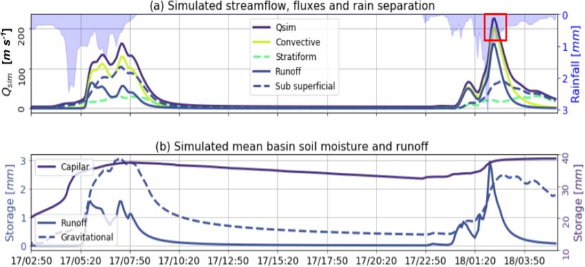
Figure 9. Summary of the results from the TETIS hydrological simulation. (a) Simulated streamflow, convective–stratiform-generated dis-
charge discrimination, and runoff and subsurface flow separation. The red square represents the flash flood peak-flow interval that is estimated
based on field campaign evidence. (b) Basin-average capillary, runoff and gravitational storages during the simulation period.
served extreme event. This section is based on the analysis duration, while gravitational storage increases considerably
of the hydrological simulation as well as the occurrence of during rain events, followed by a slow recession. There is
shallow landslides and flash floods and their simulation. A an increase in basin-wide capillary storage during Event 1,
comparison of the results from both submodels and the ob- remaining considerably high during the time leading to the
served landslide scars and flooded spots allows us to evaluate occurrence of Event 2. According to the model simulations,
the overall skill of the proposed methodology. the peak flow occurred at 02:20 LT on 18 May, which is accu-
rate compared to the reports from local authorities (between
4.1 TETIS validation and sensitivity analysis 02:10 and 02:40 LT), considering all the data limitations.
Figure 10 shows the results of a sensitivity analysis of
Figure 9a presents the results of the hydrological simula- the hydrological simulation during the second rainfall event,
tion at the outlet of the basin. The simulation shows that varying the surface speed, infiltration rate, and subsurface
Event 1 generates a hydrograph with a peak flow of Qmax = speed factors. The aim of the sensitivity analysis is to evalu-
160 m3 s−1 . It is important to note that during Event 1, there ate the robustness of the overall results, considering the fact
were no damage or flooding reports by local authorities. Even that the quality and quantity of some of the watershed in-
though this precipitation event did not generate flooding, it formation are limited. In the sensitivity analysis, we vary the
set wet conditions in the entire basin before the occurrence surface speed factor between 0.01 and 20, the infiltration fac-
of Event 2 (see the purple line in Fig. 9b representing the tor between 0.02 and 20, and the subsurface speed factor be-
capillary storage). Additionally, it is clear from the simu- tween 0.1 and 10. The overall sensitivity results show that
lation that during the flash flood event, the two successive the main findings described in the previous paragraphs are,
convective cores over the same region (training convection) in fact, robust to almost all changes in the mentioned pa-
generated a peak flow of Qmax = 220 m3 s−1 , a value that rameters, with the surface runoff associated with convective
is in the upper range of the estimated streamflow based on rainfall controlling the magnitude of the peak discharge dur-
post-event field evidence (185–222 m3 s−1 ). Figure 9a also ing Event 2. The model’s highest sensitivity, and hence the
presents the simulated runoff and subsurface flow separa- largest uncertainty source, appears to be related to the sur-
tion as well as the convective–stratiform-generated discharge face speed parameter (Fig. 10a), particularly during the peak
discrimination. The modeling evidence during Event 2 sug- flow and the early recession. On the other hand, changes in
gests the convective rainfall fraction dominates the hydro- the infiltration rate factor (Fig. 10b) and subsurface velocity
graph formation. In both events, convective (stratiform) pre- factor (Fig. 10c) are associated with simulation sensitivities
cipitation appears to be closely related to the simulated runoff smaller than 7 % and 20 % of the peak flow, respectively.
(subsurface flow). The simulated subsurface flow is more im- After the flash flood event, a stream-gauge-level station
portant in magnitude than the runoff in describing Event 1, was installed near the outlet of the basin (see Fig. 2). We use
while runoff is more relevant for Event 2. Figure 9b presents these records to validate the model results without further
not only the capillary storage (purple), but also the runoff calibration. Since the observed series correspond to stage-
(continuous blue) and the gravitational storage (dashed blue) level records, the streamflow estimation is performed follow-
temporal variability, as represented by the proposed model. ing two different approaches. The first approach, the empiri-
As expected, runoff storage is only nonzero during the storm cal one, consists of subtracting the 10th percentile of the ob-
www.hydrol-earth-syst-sci.net/24/1367/2020/ Hydrol. Earth Syst. Sci., 24, 1367–1392, 20201380 N. Velásquez et al.: Reconstructing the 2015 flash flood event of Salgar
of the basin, and the other downstream locations correspond
to 52 %, 76 %, and 100 % of the watershed. The difference
in the time of the peak discharge between the upper location
and the outlet of the basin is around 35 min, which is plausi-
ble with travel speeds between 5 and 7 m s−1 and an effective
distance of 14 km. In terms of volume, about 737 000 m3 of
the total 1 438 000 m3 simulated at the outlet of the basin is
generated in the 15 % upstream part of the watershed, cor-
responding to about half of the total mass. In terms of peak
flow, due to the slope and velocity changes, the simulated
discharge in the 15 % upstream part of the watershed cor-
responds to 50 % of the peak discharge at the outlet of the
basin.
4.2 Flash flood processes
Figure 13 presents the proposed 2-D diagrams obtained for
the simulation of the La Liboriana basin flash flood using a
spatial discretization with 50 groups. Figure 13a includes the
evolution of the average rainfall over the basin (black line)
and the spatiotemporal evolution of capillary storage (filled
isolines) and return flow (colored isolines from white to red)
by groups. For the analysis, it is relevant to highlight that
higher numbered groups are located away from the outlet of
the basin and correspond in this case to considerably steeper
Figure 10. Hydrological simulation sensitivity analysis. Similarly slopes. Figure 13b presents the evolution of streamflow at
to Fig. 9, all the panels show the simulated streamflow (purple) and the outlet of the basin (black line) as well as the gravita-
the runoff (green) and subsurface flow (dashed purple) separation. tional storage (filled isolines) and runoff (colored isolines)
From top to bottom, the panels show the simulation sensitivity to spatiotemporal evolution. Figure 13 shows variations in the
changes in the (a) surface speed, (b) infiltration rate, and (c) sub- capillary and gravitational storages associated with Event 1
surface speed factors.
in the higher numbered groups. The capillary storage remains
high in almost all the basin until the start of Event 2. Accord-
ing to the conceptualization of the model, the gravitational
served stage time series from the observational record and storage and surface runoff start to interact when the capillary
the 10th percentile of the simulated streamflow, from the storage is full. In this case, this situation is set up by Event 1.
same series. On the other hand, the second method uses the The model runs for Event 2 using dry initial states show no
Manning formula. For this, we consider the geometry of the flooding in the results.
section in Fig. 4 and the slope from the DEM. Additionally, The temporal variability of rainfall intensity plays an im-
due to the potential uncertainties, we consider three different portant role in the hydrograph structure. During Event 1,
Manning values (0.015, 0.02, 0.03). Figure 11 shows the es- rainfall accumulated over the basin at a relatively stable rate
timated streamflow using the two methods for four different (Fig. 14a). On the other hand, Event 2 presents a significant
hydrographs during July, August (two events) and Decem- increase in rainfall rate in the second half of the life cycle
ber 2015. The simulated magnitudes appear relatively close (Fig. 14b). This change in precipitation intensity is associ-
to the observations, and the peak discharge time is captured ated with a considerable enhancement of the training con-
skillfully in three of the four cases presented. The discharge vective cores due to orographic effects. Events 1 and 2 also
values using the “high” Manning number estimation (0.015) exhibit differences in the elapsed time between rainfall oc-
are similar to the empirical method. The performance of the currence and streamflow increment given the relative timing
model is acceptable (Fig. 11), considering the lack of cal- of stratiform versus convective rainfall (see the gray band
ibration, the size of the basin, and the magnitude of the in Fig. 14a and b). We compute the elapsed time between
recorded events. The results shown include cases where the the rainfall and the simulated streamflow by measuring the
peak flow was overestimated (Fig. 11c and d) and underesti- time differences between the lines for the cumulative rainfall
mated (Fig. 11b). and streamflow in Fig. 14. For Event 1, the median elapsed
Figure 12 shows the temporal evolution of discharge dur- time between rainfall and streamflow (Etp50 ) is 1.12 h, while
ing Event 2 in different locations along the watershed’s main for Event 2, Etp50 is 0.79 h. The median elapsed time be-
channel. The upper location corresponds to 15 % of the area tween the convective portion and the streamflow (Etcp50 ) in
Hydrol. Earth Syst. Sci., 24, 1367–1392, 2020 www.hydrol-earth-syst-sci.net/24/1367/2020/You can also read