Reliability-based design optimization of offshore wind turbine support structures using analytical sensitivities and factorized uncertainty ...
←
→
Page content transcription
If your browser does not render page correctly, please read the page content below
Wind Energ. Sci., 5, 171–198, 2020
https://doi.org/10.5194/wes-5-171-2020
© Author(s) 2020. This work is distributed under
the Creative Commons Attribution 4.0 License.

          Reliability-based design optimization of offshore wind
         turbine support structures using analytical sensitivities
                    and factorized uncertainty modeling
                                         Lars Einar S. Stieng and Michael Muskulus
                                  Department of Civil and Environmental Engineering,
                       Norwegian University of Science and Technology (NTNU), Trondheim, Norway
                                 Correspondence: Lars Einar S. Stieng (lars.stieng@ntnu.no)

                                  Received: 28 August 2019 – Discussion started: 4 September 2019
                       Revised: 7 November 2019 – Accepted: 15 December 2019 – Published: 29 January 2020

       Abstract. The need for cost-effective support structure designs for offshore wind turbines has led to continued
       interest in the development of design optimization methods. So far, almost no studies have considered the effect
       of uncertainty, and hence probabilistic constraints, on the support structure design optimization problem. In this
       work, we present a general methodology that implements recent developments in gradient-based design opti-
       mization, in particular the use of analytical gradients, within the context of reliability-based design optimization
       methods. Gradient-based optimization is typically more efficient and has more well-defined convergence prop-
       erties than gradient-free methods, making this the preferred paradigm for reliability-based optimization where
       possible. By an assumed factorization of the uncertain response into a design-independent, probabilistic part
       and a design-dependent but completely deterministic part, it is possible to computationally decouple the relia-
       bility analysis from the design optimization. Furthermore, this decoupling makes no further assumption about
       the functional nature of the stochastic response, meaning that high-fidelity surrogate modeling through Gaussian
       process regression of the probabilistic part can be performed while using analytical gradient-based methods for
       the design optimization. We apply this methodology to several different cases based around a uniform cantilever
       beam and the OC3 Monopile and different loading and constraint scenarios. The results demonstrate the via-
       bility of the approach in terms of obtaining reliable, optimal support structure designs and furthermore show
       that in practice only a limited amount of additional computational effort is required compared to deterministic
       design optimization. While there are some limitations in the applied cases, and some further refinement might
       be necessary for applications to high-fidelity design scenarios, the demonstrated capabilities of the proposed
       methodology show that efficient reliability-based optimization for offshore wind turbine support structures is
       feasible.

1   Introduction                                                   rotor blades and the drivetrain, wind farm layout, the elec-
                                                                   trical grid and the design of the support structure (including
Offshore wind energy is becoming an increasingly compet-           the tower). Methods to derive cost-effective, optimal support
itive alternative to the traditional land-based wind farms.        structure designs – balancing minimal use of materials (and
However, there remains a level of additional cost which, to-       potentially other cost-driving design aspects) with the ability
gether with some practical challenges, ensures that offshore       to safely withstand the loads required by design standards –
wind is still a secondary consideration in many markets.           have been an active area of research for many years. How-
Hence, the reduction of this cost is a primary objective in cur-   ever, very few studies have taken into account the probabilis-
rent research and development. Cost reduction is generally         tic, fundamentally uncertain aspects of the design process.
a multidisciplinary issue, including turbine components like       This includes, for example, uncertainties in the environment

Published by Copernicus Publications on behalf of the European Academy of Wind Energy e.V.
172    L. E. S. Stieng and M. Muskulus: Reliability-based design optimization of offshore wind turbine support structures

and the modeling of the environment, affecting the loads ex-       ies incorporating reliability-based (or otherwise probabilis-
perienced by the structure, as well as uncertainties about the     tic) approaches. For the most part, the reliability-based anal-
details of the design itself, affecting the response to the ap-    yses can be divided into two categories. Firstly, there are
plied loads. Taking such uncertainties into account generally      studies using simplified probabilistic models where the un-
requires the use of probabilistic mathematical methods that        certainty in the response is assumed to be a product of the un-
severely complicate the design optimization problem that           derlying stochastic variables and the deterministic response
needs to be solved, both formally and numerically. Hence,          variable (e.g., Thöns et al., 2010; Sørensen and Toft, 2010;
deterministic safety factors tend to be used. This is also true    Wandji et al., 2016; Yeter et al., 2016, as well as several
even for single design assessments. The present study aims         of the previously cited studies). Note that the basis for this
to address these issues by proposing a methodology that al-        kind of factorization can be justified partially or entirely de-
lows the use of both state-of-the-art optimization methods         pending on both the type of response variable and the type
recently developed for support structure design and proba-         of stochastic variable. For example, in the case of Yeter et al.
bilistic assessments of the structural response to both fatigue    (2016), the stochastic variables are mostly either modeling or
and extreme loads.                                                 simulation errors, or directly originating within the analytical
   Design optimization of structures subject to probabilistic      expressions for the response variable. Hence, the level of ap-
problem variables and parameters, sometimes called opti-           proximation involved in this kind of probabilistic modeling
mization under uncertainty, is in general a large field of re-     varies. While not strictly in the same category, studies where
search at the intersection of two larger fields, optimization      the fatigue calculation is based on crack propagation mod-
and probabilistic design. One main distinction is between          els and an assumption that the stress cycles follow a Weibull
robust design optimization (RBO) (Ben-Tal et al., 2009;            distribution, allowing exact limit state expressions to be de-
Zang et al., 2005) and reliability-based design optimiza-          rived, should be mentioned (e.g., Dong et al., 2012). Gen-
tion (RBDO) (Choi et al., 2007; Valdebenito and Schuëller,         erally, these simplifications are done in order to be able to
2010a). The main difference between the two methods is that        solve the reliability problem using first-/second-order relia-
in RBDO the design is optimized normally but under specific        bility methods (FORMs/SORMs) in a computationally fea-
probabilistic limits on structural performance (probability of     sible way. In the second category of studies, the response it-
failure), whereas in RBO the basic idea is to minimize the         self is simplified, while generally no particular assumptions
variance of a probabilistic objective function in order that the   about the stochastic nature of the response are made. This
obtained (mean) solution is robust with respect to the uncer-      has been done through static response modeling (e.g., Wei
tainties. We will generally restrict our discussion to RBDO        et al., 2014; Kim and Lee, 2015), but usually the response
and reliability methods but refer to studies on RBO and ro-        is replaced by surrogate models of some kind (e.g., Kolios,
bust methods where necessary or appropriate. Furthermore,          2010; Teixeira et al., 2017; Morató et al., 2019). The use of
given the extensive research on more general applications of       surrogate models is often done in order to be able to solve the
reliability analysis, optimization and RBDO (or optimization       reliability problem by sampling methods, generally requiring
under uncertainty more generally), we will focus on previ-         a large number of response evaluations, but surrogate mod-
ous studies concerning wind turbines. For a more expansive         els also make FORM/SORM more computationally practi-
overview of structural reliability and RBDO applied to wind        cal. Note that this division of reliability methodology is not
turbines than the one following below, the interested reader is    strict – Thöns et al. (2010) also makes use of surrogate mod-
referred to Jiang et al. (2017), Leimeister and Kolios (2018),     eling, for example – nor does it cover all approaches, but it
Hübler (2019) and Hu (2018).                                       is useful as an indicator for one of the fundamental struggles
   A substantial amount of the literature for both structural      that all the aforementioned studies have reckoned with: the
reliability analyses and RBDO of offshore wind turbines            fidelity of the probabilistic modeling vs. the fidelity of the
(OWTs) has focused on aspects other than support struc-            underlying structural analysis.
ture design. Areas such as blade design (Ronold et al., 1999;         Only a limited number of studies applying RBDO to OWT
Toft and Sørensen, 2011; Dimitrov, 2013; Hu et al., 2016;          support structure design have been made. In a series of stud-
Caboni et al., 2018), foundation design (Yoon et al., 2014;        ies, Yang and collaborators investigated optimization of a tri-
Carswell et al., 2015; Depina et al., 2016, 2017; Haj et al.,      pod support structure with probabilistic constraints. In Yang
2019; Velarde et al., 2019), component design (Kostandyan          et al. (2015), RBDO was performed, and in Yang and Zhu
and Sørensen, 2011; Rafsanjani et al., 2017; Lee et al., 2014;     (2015), RBO was performed. In both cases, a Gaussian pro-
Li et al., 2017), system/wind farm aspects (Sørensen et al.,       cess (kriging) surrogate model was used for the response and
2008), inspection and maintenance planning, and probabilis-        Monte Carlo sampling was used for the reliability calcula-
tic tuning/optimization of safety factors (Sørensen and Tarp-      tion. In Yang et al. (2018), RBDO was once again performed
Johansen, 2005; Márquez-Domínguez and Sørensen, 2012;              with a Gaussian process surrogate model, but in this case the
Veldkamp, 2008) have all been studied. As for support struc-       reliability calculation was done using a fractional moment
ture design specifically, though most structural analyses of       method in order to reduce the number of system evaluations
OWTs remain deterministic, there has been a number of stud-        required. All three studies used the heuristic optimization

Wind Energ. Sci., 5, 171–198, 2020                                                        www.wind-energ-sci.net/5/171/2020/
L. E. S. Stieng and M. Muskulus: Reliability-based design optimization of offshore wind turbine support structures           173

method called the multi-island genetic algorithm, and the re-     2018 for a comparison of these three approaches and a more
liability calculations were done for each step in the optimiza-   thorough review of support structure optimization). In gen-
tion loop, creating a nested two-loop structure. As one might     eral, these approaches make the design optimization problem
expect from a heuristic method, the number of iterations re-      more efficient and stable, though, because of the added con-
quired to solve even the deterministic optimization problem       ceptual complications, these methods have yet to be applied
(around 300 iterations) is rather large given the small number    in studies considering a more realistic and comprehensive set
of design variables used, and this is much more pronounced        of loading conditions. A study founded on gradient-based op-
in the case of the stochastic optimization (around 3000 itera-    timization that does consider a more comprehensive set of
tions). This means that the method is rather computationally      loading conditions but does not utilize analytical sensitivities
inefficient, especially considering the number of system eval-    was performed by Häfele et al. (2019). They used a Gaussian
uations required by the reliability calculation and the genetic   process surrogate model to simplify the response, thus mak-
algorithm at each iteration. However, due to the use of the       ing the analysis computationally feasible. This study also
surrogate model, this practical issue is overcome, if still ap-   used a more complicated and (arguably) more realistic objec-
parent. Though not an application to OWTs, it is also worth       tive function, modeling the cost of the support structure in a
mentioning the study of RBDO applied to offshore mono-            more detailed way than the strictly steel mass-/volume-based
pod towers in Karadeniz et al. (2010b) and applied to jacket      approaches that are otherwise commonly used. However, it
structures in Karadeniz et al. (2010a). Here, the limit state     was seen that, at least with the particular cost formulations
functions are formulated analytically, and a nested two-loop      used, the solution was more or less the same as when a sim-
approach using gradient-based optimization (in this case se-      pler mass-based objective function was used. Another recent
quential quadratic programming, SQP) and FORM is used.            study regarding deterministic support structure optimization
   The previous work on RBDO for OWTs (for both sup-              was done in Couceiro et al. (2019). Like the previous study,
port structures and otherwise) demonstrates that these meth-      completely analytical sensitivities were not used. The plau-
ods can obtain optimal designs that are both more robust/safe     sibility of more comprehensive code checks for design op-
with respect to uncertainties than designs optimized under        timization under dynamic loading was in this case demon-
deterministic criteria and more tailored to specific design       strated by a simplified fatigue extrapolation procedure and
conditions than deterministic designs using safety factors.       an aggregation of time-dependent stress constraints (for ul-
However, so far (and this is particularly true for support        timate limit state analysis) into a single constraint per stress
structure designs), no studies have taken advantage of recent     time series. All these studies have been focused on bottom-
advances in deterministic structural optimization methodol-       fixed structures (jackets in particular, though the methodolo-
ogy. Optimization methods in general can be divided into          gies are easily transferable to monopiles) and it is unclear
gradient-based and gradient-free (often heuristic) methods.       what level of adaptation is necessary to extend these formu-
Both approaches have been applied to support structure de-        lations to floating structures.
sign and other wind turbine components (both on- and off-            As seen in several of the cited studies above, the use of
shore). With some exceptions (e.g., Negm and Maalawi,             surrogate modeling to simplify the response analysis has be-
2000 using an interior penalty method), gradient-free meth-       come more common recently. For optimization and reliabil-
ods were the most common among earlier studies. Examples          ity analysis, and all the more so for RBDO, this is a natural
include Yoshida (2006) using a genetic algorithm, Uys et al.      way to make the problems more computationally tractable
(2007) with a Rosenbrock search and Zwick et al. (2012)           when faced with having to perform a large number of time-
with a local scaling of sectional members. The advantages of      consuming simulations. However, surrogate modeling is in-
these approaches are that no gradient information is needed       creasingly also proposed for basic structural analysis due to
for the optimization, which simplifies the calculations that      the large number of environmental states that need to be
need to be performed for each iteration and avoids the re-        checked for certification according to design standards (e.g.,
liance on finite difference methods, which can be unstable        International Electrotechnical Commission, 2009). For ex-
in some implementations. On the other hand, these meth-           ample, Toft et al. (2016a) used a response surface based on
ods, at least when done at a similar level of detail, gener-      Taylor expansions, and Gaussian process regression was used
ally converge much slower than gradient-based alternatives,       by Huchet et al. (2019) and Teixeira et al. (2019) for fa-
where the search for optimal designs can be more specifically     tigue design and by Abdallah et al. (2019) for ultimate limit
guided by the information provided by the gradients. With         state (ULS) design. Though there are some challenges re-
this disadvantage of gradient-free methods in mind, and seek-     garding the number of samples required to build an accurate
ing to avoid the issues related to finite difference methods,     model, this can be alleviated by efficient design of experi-
some recent studies have demonstrated the viability and, in       ment and/or adaptive methods. The overall indication seems
most cases, advantages of analytical sensitivities in gradient-   to be that surrogate modeling, and particularly Gaussian pro-
based formulations. This has been shown for static (Sandal        cess regression, provides a viable strategy for simplifying the
et al., 2018), quasi-static (Oest et al., 2017) and dynamic       structural analysis in design problems.
(Chew et al., 2016) loading conditions (see also Oest et al.,

www.wind-energ-sci.net/5/171/2020/                                                        Wind Energ. Sci., 5, 171–198, 2020
174    L. E. S. Stieng and M. Muskulus: Reliability-based design optimization of offshore wind turbine support structures

   In summary, while considerable work has gone into im-           ther discussion section; and a summary and final thoughts, in
proving the various analyses and methods involved in RBDO          the conclusions.
for support structures, there is a very limited amount of stud-
ies that connect these pieces together. In particular, the work    2     Methodology
on analytical design sensitivities has not been implemented
into RBDO, nor has it been combined with surrogate mod-            In the following, we present the basic framework of (deter-
eling approaches that make more comprehensive structural           ministic) design optimization for OWT support structures.
analysis and/or reliability analysis computationally feasible.     Then, some aspects of RBDO and surrogate modeling are ex-
These gaps are what we intend to explore in the present            plained. Finally, the synthesis of these aspects resulting in the
study. By a very particular formulation of the probabilistic       proposed RBDO methodology is motivated and presented.
constraints (limit state functions) used for the support struc-
ture design optimization, we demonstrate how these con-            2.1       Design optimization of offshore wind turbine support
straints can remain analytically differentiable with respect to              structures
the design variables while at the same time using a surro-
gate model for the stochastic variation of the response. By        For the task of finding the minimum structural mass fmass
doing so, we retain the advantages of the state-of-the-art de-     of a topologically fixed design consisting of N circular cross
terministic optimization formulations while ensuring that the      sections, the following optimization problem can be formu-
uncertainties are propagated through the system in a way that      lated:
makes less simplifications than the commonly used factoriza-           minfmass (x)      such that
tion approaches and without incurring substantial additional            x
computational effort. By assuming that some kind of fac-           Alin x ≤ b
torization of the response is valid locally in design space,                x ≤ xu
a standard double-loop RBDO formulation can be applied
                                                                            x ≥ xl
together with a design-independent Gaussian process surro-
gate model that makes the inner loop used to solve the reli-       cj (x) ≤ 0        ∀j ∈ J .                                    (1)
ability problem computationally insignificant. Retraining the
                                                                   Here, x are the design variables, Alin and b give rise to a sys-
surrogate model and repeating the optimization a few addi-
                                                                   tem of linear inequality constraints, x u and x l are upper and
tional times then leads to convergence and an optimal de-
                                                                   lower bounds, respectively, and cj represents a non-linear
sign that is feasible with respect to uncertainties in both the
                                                                   constraint function indexed according to some set J . The de-
loads and the structural modeling. In addition to incorporat-
                                                                   sign variables for this problem will be the diameters Di and
ing more advanced optimization methods to the RBDO prob-
                                                                   thicknesses ti of each cross section i ∈ {1, . . ., N }. The total
lem than has been done previously for OWT support struc-
                                                                   mass of all N cross sections is calculated as
ture design, the current approach can also be seen as a natural
middle ground between, on the one hand, the simplified an-                                       N
                                                                                                 X
alytical limit state formulations and, on the other hand, the      fmass (x = (D; t)) = πρ             Li (Di ti − ti2 ),        (2)
                                                                                                 i=1
completely surrogate-model-based limit state formulations,
the two most commonly used approaches in reliability anal-         where Li represents the (constant) length of each structural
ysis and RBDO for OWTs previously.                                 element with cross sections given by Di and ti , and ρ is the
   The structure of the paper from this point on is as fol-        material density (assuming a uniform density throughout the
lows. In the first section (methodology), the general theoreti-    structure). Examples of the type of linear constraints that can
cal background is presented first, with focus on optimization,     be represented by Alin x ≤ b are limits on the ratio of each
reliability analysis and RBDO, but some details about surro-       Di to each ti (the D − t ratio). The non-linear constraint cj
gate modeling are also included. The section is concluded          typically corresponds to safety criteria for ULS and the fa-
with a motivation and presentation of the proposed method          tigue limit state (FLS) but often also includes constraints on
from a general point of view. The next section (testing and        the first eigenfrequency of the structure.
implementation details) describes the setup for how we have           The optimization problem in Eq. (1) can be solved either
chosen to test the method in practice. This includes specific      by gradient-based or gradient-free (heuristic) methods. All
models and what kinds of loads are included, the type of con-      gradient-based methods require, as the name suggests, the
straints included in the optimization, sensitivity analysis and    calculation of the gradients of the problem. In a constrained
uncertainty modeling. Additionally, some particular practi-        problem like Eq. (1), that means estimating the gradients of
cal details of how the method has been implemented are dis-        both the objective function fmass and all the constraints. For
cussed. The remaining sections of the paper include a pre-         an objective function like the one stated in Eq. (2) and for
sentation and discussion of the results, in the results section;   any linear constraints, this is a trivial problem. For non-linear
more detailed treatment of a few points of interest, in the fur-   constraints, the calculation of gradients (often called sensitiv-
                                                                   ities in the optimization field) can be very difficult, especially

Wind Energ. Sci., 5, 171–198, 2020                                                              www.wind-energ-sci.net/5/171/2020/
L. E. S. Stieng and M. Muskulus: Reliability-based design optimization of offshore wind turbine support structures                175

when the value of these constraints depends on output from         rule and finally the solution of Eq. (4). It is presently assumed
simulations, as is generally the case for support structure op-    that the system matrices (M, C and K) are known analyti-
timization. This difficulty can in principle be accommodated       cal functions of the design variables, as is the case when the
by the use of finite difference methods, where the function        structural analysis is based on finite element modeling with
values around the current design point are used to get an es-      beam elements defined according to Euler or Timoschenko
timate of the gradient. However, the use of finite difference      beam theory. If this is not the case, the use of semi-analytical
methods can lead to inaccurate solutions or failure to con-        methods (where the gradients of the system matrices are es-
verge, or will at least often require a larger number of func-     timated with finite differences) must be used. For OWT sup-
tion evaluations (computationally costly when simulations          port structures, it was shown in Chew et al. (2016) how the
are needed for each such evaluation) to obtain the same solu-      sensitivities of both ULS and FLS constraints could be ob-
tion as one would using the exact gradients (see, e.g., Chew       tained using the analytical approach described above.
et al., 2016). Additionally, the accuracy of finite difference
estimates depends strongly on the chosen step size, the opti-
mal value of which again depends strongly on the (possibly         2.2    RBDO
local) properties of the function in question (see, e.g., Press    The main distinguishing feature, with respect to the prob-
et al., 2007 for a general discussion and Oest et al., 2017 for    lem structure defined in Eq. (1), of optimization under uncer-
a demonstration of this effect for support structure design).      tainty, is the addition of a new set of stochastic variables θ
Hence, it is desirable to use analytical sensitivities whenever    that in general can enter both the objective function and the
possible. Examples of common heuristic methods are genetic         constraints. In fact, some or all of the design variables in x
algorithms, particle swarm algorithms and random search.           could be replaced (or depend on) variables in θ . However, in
The reason that these methods might be used over gradient-         our case, we shall restrict the discussion to cases where all
based methods is that no estimation of sensitivities is neces-     the design variables are deterministic. It follows that the only
sary in that case, seemingly avoiding the problem described        θ dependence must then be in the so far to be determined
above related to gradient estimation. However, as a trade-off,     non-linear constraints cj . In RBDO, the main idea is that we
these gradient-free methods generally require a much larger        seek to constrain (and/or, in some formulations, optimize)
number of iterations to convergence to the solution, since the     the reliability of the system. The reliability of a structural
methodology is typically founded on some kind of loosely           system is a probabilistic measure of its ability to resist loads.
guided (possibly random) search of the parameter space.            In the most straightforward mathematical representation, this
While being able to overcome some of the weaknesses of             is expressed as the extent to which the load effect Q (usually
gradient-based optimization, for simulation-based problems,        depending on the response) does not exceed the resistance R
the resulting added computational expense of heuristic meth-       (usually depending on the capacity or structural strength). In
ods might not be acceptable in practice. Since the gradient-       a probabilistic setting, this is quantified by the probability of
based methods using analytical sensitivities are able to avoid     failure Pf , defined as
the numerical issues associated with finite differences and
obtain accurate gradient information, these methods are con-       Pf = Prob(Q − R > 0).                                           (5)
sequently preferable. Hence, we shall focus our attention on
gradient-based methods from this point onwards.                    Formally, the reliability is the probability of non-failure,
   It is a well-known result (see, e.g., Kang et al., 2006) that   1 − Pf , though commonly one tends to use Pf rather than the
when the displacements u(t) of the structural system under         actual reliability in analysis and calculations. Furthermore,
dynamic loading S(t) are found by time integration of the          since the analogy of load effect and resistance is not always
equation of motion, given as                                       applicable, the notion of failure is usually represented by a
M(x)ü(t) + C(x)u̇(t) + K(x)u(t) = S(t),                    (3)    limit state function g, encoding failure as positive function
                                                                   values, with the probability of failure as
for mass matrix M, damping matrix C and stiffness matrix
K, then the sensitivities of the displacements can be found        Pf = Prob(g > 0).                                               (6)
by time integration of the following equation:
                                                                   In general, g is a function of both x and θ , and to calculate
     dü(t)         du̇(t)         du(t) dS(t)
M(x)        + C(x)         + K(x)        =                         Pf requires knowledge of the joint probability distribution hθ
      dx              dx             dx     dx                     of all the stochastic variables in θ . An exact estimate of Pf is

      dM(x)            dC(x)         dK(x)                         then given by the integral of hθ over the part of its domain
  −           ü(t) +        u̇(t) +       u(t) .           (4)
         dx             dx             dx                          where g > 0, i.e.,
Hence, if the non-linear constraints can be expressed as an-                 Z
alytical functions of the displacements, the sensitivities are     Pf =               hθ (θ 0 )dθ 0 .                              (7)
obtainable via (possibly repeated) application of the chain               g(x,θ )>0

www.wind-energ-sci.net/5/171/2020/                                                                  Wind Energ. Sci., 5, 171–198, 2020
176        L. E. S. Stieng and M. Muskulus: Reliability-based design optimization of offshore wind turbine support structures

The general RBDO problem may then be formalized as                  where 8−1 is the inverse of the standard normal cumula-
                                                                    tive distribution function (CDF), Hθi is the CDF of θi , and
   minfmass (x)       such that                                     I is the set of all the indices for the stochastic variables in θ.
      x
                                                                    This particular transformation assumes that the variables in
 Alin x ≤ b                                                         θ are independent, which is not always the case. For non-
          x ≤ xu                                                    independent stochastic variables, a slightly more involved
          x ≥ xl                                                    transformation (e.g., the Rosenblatt transformation; Rosen-
                                                                    blatt, 1952) must be used. By substituting v for θ in g, we ob-
 cj (x) ≤ 0        ∀j ∈ Jdet
             max
                                                                    tain g(x, v). We want to linearize this function at the point on
Pf,j (x) ≤ Pf,j       ∀j ∈ Jprob ,                           (8)    the boundary between failure and non-failure, g = 0, that is
                                                                    closest to the origin in standard normal space, the most prob-
where Jdet and Jprob represent the indices of deterministic         able point (MPP) on the failure surface. This can be found by
and probabilistic constraints, respectively, and Pf,jmax are the
                                                                    solving the following optimization problem:
desired upper bounds on the probabilities of failure Pf,j .             sX
   However, for any but the most trivial limit state functions,     min        vi2 such that
the determination of the values of x and θ giving g > 0, and         v
                                                                            i
hence the determination of the integral in Eq. (7), cannot be
done exactly. The most straightforward and robust way to ac-             g(x, v) = 0.                                            (10)
commodate this is through the use of sampling methods. In           We denote the optimal point solving the above vq   ∗ , and the
particular, the family of Monte Carlo and quasi-Monte Carlo                                                               P ∗2
methods is typically used. These methods generally have the         corresponding minimal distance to the origin β =        i (vi )
property that for a large enough sample size, the resulting es-     is called the reliability index. The probability of failure is
timate Pbf tends towards the exact value of Pf . Unfortunately,     then estimated as Pf = 8(−β). Some care must be taken
large enough can be an intractable requirement. While the           in the application of FORM methods, since this represen-
use of variance reduction techniques can speed up the conver-       tation is only exact in the case that g is a linear function.
gence, as the dimensionality and complexity of the problem          For a non-linear g, FORM is an approximation, but it is
grows, the number of samples does too. This can be particu-         often good enough for many engineering applications. Be-
larly problematic when one or more simulations are required         yond merely offering a tractable solution to Eq. (7), there
for each sample. Furthermore, sampling methods do not nat-          are several properties that make FORM desirable for RBDO.
urally lend themselves well to gradient-based optimization          Consider, for example, the behavior of the probabilistic con-
due to the additional effort involved in the calculation of the     straints in Eq. (8). Pf will tend to vary over many orders of
gradients of a quantity estimated by sampling. In some cases,       magnitude, which can be detrimental to the behavior of many
when the design variables are stochastic, the use of what is        algorithms for gradient-based optimization. The introduction
called score functions for the estimation of design sensitivity     of the reliability index means that we can replace the con-
is possible, in which case no additional samples are needed         straints involving Pf with equivalent ones involving β, i.e.,
(see, e.g., Hu, 2018). At the very least, no analytical gradients
                                                                    βj ≤ βjmax = −8−1 (Pf,j
                                                                                         max
                                                                                             ).                                  (11)
can be obtained. Hence, it is common to make use of first-
and second-order approximations of the limit state function,        This substitution has a further advantage when calculating
making integration over the g > 0 region feasible.                  sensitivities. Even without an explicit expression for the
                                                                    derivative of Pf with respect to x, we can make the following
                                                                    observation. In the two cases where the design x is such that
2.2.1      FORM                                                     the region g > 0 is either very small (very safe designs) or
The objective of FORM is to approximate the non-linear fail-        very large (very unsafe designs), the change in Pf due to a
ure surface, the set of points such that g > 0, by a linear         small change in x is virtually zero. Hence, in these design
function of independent standard normal variables v, derived        configurations, the sensitivity vanishes, which has a detri-
from the original set of stochastic variables θ. Historically,      mental effect on the optimization since most algorithms will
there have been several versions of FORM and related meth-          struggle to find new candidate points that lead to measurable
ods (see, e.g., Choi et al., 2007 and Enevoldsen and Sørensen,      changes in the constraints. Using β as the constraint function
1994, where also more details about FORM in general can             instead gives the following, generally non-vanishing, expres-
be found), but we shall restrict the discussion to the one most     sion (Enevoldsen and Sørensen, 1994):
commonly used. The main idea is as follows: construct the           dβ   1 dg
set of independent standard normal variables v = {vi } by ap-          = dg    .                                                 (12)
                                                                    dx      dx
plying the transformations                                                  dv
                                                                       However, one problem with the definition of FORM given
vi = 8−1 (Hθi (θi ))     ∀i ∈ I,                             (9)    in Eq. (10), typically called the reliability index approach

Wind Energ. Sci., 5, 171–198, 2020                                                          www.wind-energ-sci.net/5/171/2020/
L. E. S. Stieng and M. Muskulus: Reliability-based design optimization of offshore wind turbine support structures                       177

(RIA), is that it is not always possible to find a configuration
v such that g = 0 (within a sufficiently small tolerance). This
can lead to slower convergence of the RBDO problem or in
the worst cases a lack of convergence at all. To resolve this
issue, it is possible to formulate an inverse problem where
instead of calculating the reliability index for a given de-
sign, one finds the configuration of v giving the smallest ex-
ceedance of g > 0 for a given (fixed) reliability index. This
is called the performance measure approach (PMA) and will
be explicated below.
                                                                     Figure 1. The difference between the solutions provided by RIA (a)
2.2.2     PMA                                                        and PMA (b) for a linear limit state function g with two variables,
                                                                     (v1 , v2 ) = v, in standard normal space. The target reliability index
The main idea of PMA is to reverse the role     of objective and     for PMA (βt = 3.3) is higher here than the RIA solution (β = 2.28),
                                                                     so the PMA solution finds g ∗ > 0. Also indicated are examples of
                                             qP
constraint in Eq. (10). If we demand that            2     max as
                                                  i vi = β           points visited during the respective optimizations (initial, v 0 , inter-
a constraint, we can instead find the largest possible value of      mediate, v k , and solution points, v ∗ ; different for the two methods),
g for which that constraint is satisfied. In other words,            where the displayed points before the solution are feasible but not
                                                                     optimal.
max g(x, v) such that
 v
sX
    vi2 = β max .                                            (13)    where g ∗ = 0 for the final solution. However, if one wishes
    i                                                                to compare the probability of failure of such an optimized
                                                                     design with the corresponding initial design or a design opti-
If we again call the solution point v ∗ and term the corre-          mized by deterministic methods, then PMA does not imme-
sponding value of g as g ∗ , then, under the assumptions of          diately provide a quantitative answer. It only provides a qual-
the validity of FORM, it follows that Prob(g > g ∗ ) = Pfmax .       itative assessment of whether or not the probability of failure
Hence, by further demanding that g ∗ ≤ 0, we can guaran-             is above or below the given threshold. To get a quantitative
tee that Pf ≤ Pfmax . The optimization problem in Eq. (13) al-       assessment in these cases, we can exploit the approximate
ways has a solution. Aside from the robustness provided by           linearity of g ∗ , especially close to g ∗ = 0. If we have solved
this, PMA has a few other advantages. For example, it can be         the PMA problem in Eq. (13) once for a target reliability βt ,
shown that (see, e.g., Frangopol and Maute, 2005)                    obtaining the solution g ∗ , we can then use the secant method
                                                                     to construct an estimate of β0 ≡ β(g ∗ = 0) as
dg(x, v ∗ ) ∂g(x, v ∗ )
           =            ,                                    (14)
   dx          ∂x                                                                βt − β 0 ∗
                                                                     β0 = βt −              g ,                                         (16)
which simplifies the sensitivity analysis. More generally, for                   g ∗ − g 0∗
applications to RBDO, PMA tends to perform better (Tu
                                                                     where g 0∗ is the solution of a PMA problem for a target relia-
et al., 1999; Youn and Choi, 2003; Lee et al., 2002). An il-
                                                                     bility β 0 ∈ (βt , β0 ). If the initial g ∗ is sufficiently small (close
lustration of the difference between RIA and PMA is made
                                                                     to 0) and/or sufficiently linear, then the above will provide
in Fig. 1.
                                                                     a good estimate β0 and hence an estimate of the probability
   The RBDO problem using PMA can be stated as
                                                                     of failure as Pf = 8(−β0 ). Otherwise, this procedure can be
        minfmass (x)   such that                                     iterated (setting βt = β 0 and β 0 = β0 ). In such cases, unless
         x                                                           the initial g ∗ is very far away from zero and/or g is highly
    Alin x ≤ b                                                       non-linear, only a few more iterations (1–3) should suffice to
          x ≤ xu                                                     get at least two digits of accuracy for Pf .
          x ≥ xl
                                                                     2.2.3    Two-loop RBDO vs. single-loop RBDO
    cj (x) ≤ 0     ∀j ∈ Jdet
gj (x, v ∗ ) ≤ 0   ∀j ∈ Jprob .                              (15)    As is evident from Eq. (15), the current formulation of the
                                                                     RBDO problem consists of two nested loops. One outer op-
where each gj solves Eq. (13) with β max = −8−1 (Pf,j       max ).   timization problem that solves the design optimization prob-
One potential downside of PMA is that it does not provide            lem under the given constraints and one inner optimization
a direct estimate of the probability of failure. This is fine for    that solves the (PMA) reliability problem to obtain the prob-
optimization, where being below the threshold is sufficient          abilistic constraints for each iteration. This can be computa-
and where at least one constraint should be at the boundary          tionally demanding, even when the convergence of the PMA

www.wind-energ-sci.net/5/171/2020/                                                                Wind Energ. Sci., 5, 171–198, 2020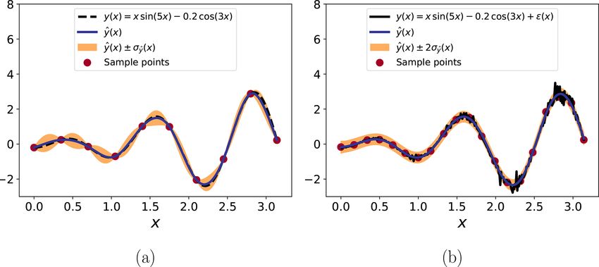
178    L. E. S. Stieng and M. Muskulus: Reliability-based design optimization of offshore wind turbine support structures

subproblem is accelerated by the use of improved optimiza-           2.3.1   GPR
tion methods like the hybrid mean-value algorithm (Youn
                                                                     The essentials of GPR are quite similar to conventional re-
et al., 2003). For this reason, several alternative solution
                                                                     gression methods. We wish to construct a model y(x) for the
strategies for RBDO have been proposed (Valdebenito and
                                                                     response y to some input x. However, instead of consider-
Schuëller, 2010b). This usually involves either decoupling
                                                                     ing, for example, a multi-linear or polynomial model plus a
the two loops into a sequence of deterministic optimization
                                                                     simple noise term, one instead considers a more general ex-
and reliability analysis, most prominently in the sequential
                                                                     pansion of the input in some basis B (which could be con-
optimization and reliability analysis (SORA) method (Du
                                                                     stant, linear, polynomial or otherwise) plus a realization of a
and Chen, 2004), or the use of reformulated single-loop
                                                                     zero-mean Gaussian process (GP):
approaches, most prominently in the aptly named single-
loop approach (SLA) (Chen et al., 1997). All these meth-             y = γ B(x) + GP(x),                                           (17)
ods involve some kind of approximation of the FORM-based
constraint. While speeding up the convergence significantly          where γ is a set of basis coefficients. The Gaussian process is
compared to conventional two-loop strategies, this can also          determined by its covariance function, which is the product
lead to lack of convergence for some problems (Aoues and             of the noise parameter σ and a kernel function. The kernel
Chateauneuf, 2010). On the other hand, SORA seems to be              function gives the covariance function its main structure by
fairly robust, due in large to the fact that its reliability-based   determining the correlation between points (x, x 0 ). Usually,
constraint is locally equivalent to the two-loop approach,           these kernel functions are exponentially decaying with the
meaning that as the changes in the design become small from          Euclidean distance between the points. In addition to σ , the
one round of deterministic optimization to the next, the error       covariance function is parameterized by one or more hyper-
in the approximation when using a fixed reliability estimate         parameters. All in all, GPR consists of fitting γ , σ and all
during the design optimization tends to zero.                        the kernel parameters based on a set of training data {yi , xi },
                                                                     where in general each input xi can be multi-dimensional.
2.3   Surrogate modeling                                             These parameters are fit using maximum likelihood estima-
                                                                     tion, though finding optimal parameters often requires the
Surrogate modeling is generally a vast topic and the inter-
                                                                     use of global optimization methods in order to fully con-
ested reader is referred to Wang and Shan (2006) and Mars-
                                                                     sider the range of possible parameter values. The fitted co-
land (2015) for more general overviews, as well as to Tunga
                                                                     variance function of the GPR model, in particular the value
and Demiralp (2005) for the high-dimensional model repre-
                                                                     of σ , provides a natural estimate of the inherent uncertainty
sentation approach and Rasmussen and Williams (2006) and
                                                                     (or expected error) of the surrogate model, which can then
Santner et al. (2018) for more detailed looks at Gaussian pro-
                                                                     be used to establish confidence/prediction intervals for pre-
cess regression (GPR). For applications to RBDO in general,
                                                                     dicted model responses to new inputs. An illustration of GPR
Dubourg (2011) and Jin et al. (2003) are instructive.
                                                                     is given in Fig. 2.
   Focusing our attention to wind turbine applications, it has
been common for quite some time to use surrogate model-
ing due to the computationally demanding simulations re-             2.3.2   Design of experiment
quired for time-domain analysis. This is especially true for         As noted previously, GPR can require a large number of sam-
reliability analysis, optimization and RBDO, due to the dras-        ples to attain its desired fidelity. For this reason, it is common
tically increased computational effort involved. The most            to apply specialized sampling techniques, together usually
commonly applied types of surrogate models in wind energy            referred to as the design of experiment (DOE), that sample
have been response surface models (typically second-order            the input space more efficiently and thereby require less sam-
polynomials), Taylor expansions and (especially more re-             ples than, e.g., uniform random sampling. Depending on the
cently) GPR. GPR has many advantages, including the abil-            desired outcome, one could, for instance, opt for importance
ity to capture non-linearities with higher fidelity and provid-      sampling (most useful in this case if it is known that only a
ing an estimate of its own uncertainty by default but gener-         certain region of the input space is of interest, e.g., for a reli-
ally requires a larger number of samples to gain a significant       ability analysis where one mainly wishes to use the surrogate
advantage over response surface methods (Kaymaz, 2005).              model around the failure surface) or a space-filling approach
We note that GPR is often referred to as kriging in the engi-        like Latin hypercube sampling or quasi-Monte Carlo sam-
neering literature. Although, for most practical purposes, the       pling (these are most useful when as wide coverage of the in-
two terms can be used interchangeably, GPR is more general.          put space as possible is needed, e.g., for optimization where
Hence, to avoid specificity where it is not needed, we will use      the region of interest is likely to shift dynamically). A com-
the term GPR.                                                        parison between Latin hypercube sampling and quasi-Monte
                                                                     Carlo sampling was performed in Kucherenko et al. (2015),
                                                                     where it was found that Latin hypercube sampling can give
                                                                     better or more efficient results for certain types of problems

Wind Energ. Sci., 5, 171–198, 2020                                                           www.wind-energ-sci.net/5/171/2020/
L. E. S. Stieng and M. Muskulus: Reliability-based design optimization of offshore wind turbine support structures                   179

                                                                            What can be concluded from this? Simply put, consider-
                                                                         able progress could be made by making the state of the art
                                                                         for OWT RBDO, and for support structure design in par-
                                                                         ticular, more in line with the general state of the art. How-
                                                                         ever, this should be done in a way that maintains some of
                                                                         the OWT-specific developments made in previous optimiza-
                                                                         tion studies. Furthermore, by combining elements from all
                                                                         these sources, it could be possible to obtain a synthesized
                                                                         methodology that retains many of the individual advantages.
                                                                         However, this requires a new approach because of the ways
Figure 2. GPR demonstrated on two related test functions: one with       in which the previous methods seem incompatible. It is, e.g.,
no noise (a) and one with noise (b). In the former case, 10 sample       seemingly not possible to use analytical sensitivities if the
points are enough for a very good estimate (the real function, y,        simulation output is replaced by surrogate models.
being within 1 standard deviation of the estimate, ŷ, throughout).
Note also how the uncertainty decreases around the sample points in
this case due to the lack of noise. In the second case, more samples
                                                                         2.4.2    Key simplification
are needed for a good estimate. The noisy function does at one point     Suppose that all relevant limit state functions gj can be writ-
exceed even 2 standard deviations away from the estimate, but the        ten in the form gj = Q − R, which is generally the case for
underlying (non-noisy) function is well estimated. Note also how
                                                                         support structure design, with Q and R being the load effect
the uncertainty level, while more or less constant, is not higher than
it was away from the sample points of the non-noisy case.
                                                                         and resistance as before. Furthermore, for simplicity (and
                                                                         since this is usually the case), assume that while both Q and
                                                                         R are functions of the design x and the stochastic variables
but that quasi-Monte Carlo sampling was otherwise equal or               θ , only Q is determined by simulations. We then make the
superior and generally more robust when the problem could                following simplification:
not be classified a priori. Latin hypercube sampling has been            Q(x, θ ) = Y (θ)Q̃(x),                                      (18)
more common for wind energy applications, but a quasi-
Monte Carlo sampling method based on the Sobol sequence                  where Y is some arbitrary unknown function with the prop-
was used in Müller and Cheng (2018).                                     erty that Y (θ ) = 1, with θ as the mean values of θ , and
                                                                         Q̃(x) = Q(x, θ ) is the mean response at the specific design
                                                                         x. A simple example of how such a factorization makes
2.4     Proposed RBDO framework
                                                                         sense locally is shown in Fig. 3. What are the implica-
In the following, we will explain the details of our proposed            tions of this assumption? Firstly, note that this assumption
framework for RBDO of OWT support structures. However,                   is consistent with the common simplified limit state func-
we begin with a few remarks that serve to motivate this ap-              tions where the stochastic response is modeled as the prod-
proach.                                                                  uct of the stochastic variables θ and the design-dependent
                                                                         mean response. However, in our case, we make no assump-
2.4.1    Motivation                                                      tion about the functional representation of this factorization.
                                                                         Hence, this should allow for a higher-fidelity representation
Considering the state of the art for reliability analysis and            of how stochastic variables input to the system are propa-
RBDO for OWTs more generally, we can make a few sum-                     gated through the response estimation. Secondly, while this is
mary observations based on the previous discussion. Firstly,             indeed a simplification which cannot in general be assumed
the vast majority of studies make use of either simplified an-           valid, previous studies detailing how the fatigue damage dis-
alytical limit state functions (allowing more easily the use             tribution of OWT support structures changes when the design
of FORM and making the probabilistic constraints easier                  is modified (Stieng and Muskulus, 2018, 2019) indicate that
to combine with design optimization) or surrogate models                 this kind of proportional scaling is a reasonable assumption
that completely replace simulation output (usually combined              as long as the design does not change too much. Further-
with sampling-based reliability analysis). Secondly, when                more, it is not unreasonable to make a similar assumption for
not based on heuristic optimization methods (as has been                 extreme loads. Thirdly, this factorization makes it possible
the case for all RBDO studies concerning the design of sup-              to fit a surrogate model of the response to variations in the
port structures specifically), gradient-based design optimiza-           stochastic variables only, while the design-dependent part of
tion as part of RBDO has not utilized analytical sensitivities.          the response remains as in a deterministic setting. On the one
Thirdly, little to no use of PMA for reliability analysis or             hand, this means that we can fix the design and fit our surro-
more advanced RBDO methods like SORA or SLA has been                     gate model as
made, despite their notable advantages.
                                                                                      Q(x, θ s )
                                                                         Y (θ s ) =                ,                                 (19)
                                                                                       Q̃(x)

www.wind-energ-sci.net/5/171/2020/                                                                     Wind Energ. Sci., 5, 171–198, 2020
180     L. E. S. Stieng and M. Muskulus: Reliability-based design optimization of offshore wind turbine support structures

                                                                              minfmass (x)      such that
                                                                               x
                                                                            Alin x ≤ b
                                                                                   x ≤ xu
                                                                                   x ≥ xl
                                                                            cj (x) ≤ 0      ∀j ∈ Jdet
                                                                        gj (x, v ∗ ) ≤ 0    ∀j ∈ Jprob .

                                                                        gj is now defined as
Figure 3. An example of factoring out the dependence of one vari-
able from a non-separable expression by using GPR to fit this un-       gj (x, θ ) = yj (θq )qj (x) − rj (x, θr ),               (21)
known factor. The figure shows the relative error when approximat-
                                                                        with yj as a surrogate model defined and fit according
ing (x + y)2 as f (y)(x + 1)2 , around x = 1, with f (1) = 1 and oth-
erwise unknown. Note the accuracy of this representation around
                                                                        to Eqs. (18) and (19), and θq and θr are the stochastic
(1,1) and in general the moderate error level as we move away from      parameters in θ for the load effect and the resistance,
this region.                                                            respectively. Note that we can obtain θi = Hθ−1 i
                                                                                                                          (8(vi )), so
                                                                        that even though the solution of the reliability subproblem
                                                                        resulting in v ∗ is performed in standard normal space, it is
where for each sampled point θ s we estimate the total re-              never necessary to obtain yj as a function of v. To ensure
sponse Q and then factor out the design-dependent mean re-              that the RBDO problem is solved with sufficient accuracy,
sponse. This greatly reduces the dimensionality of the surro-           specifically that the final design is actually feasible with
gate modeling problem, since we do not have to also sam-                respect to the probabilistic constraints, the procedure can
ple different values of x. Since the fit is design independent          be repeated several times, fitting a new surrogate model at
given the underlying simplifications, we may then say that              the solution of the previous RBDO loop and starting a new
we obtain a quasi-global (in design space) surrogate model              RBDO loop from this design point. The overall method is
that can be used throughout a design optimization procedure,            compactly stated as Algorithm 1 and illustrated in Fig. 4.
greatly reducing the computational effort of any reliability
calculation. On the other hand, the separation of stochastic
and deterministic response means that for the estimation of
design sensitivities we have the property that

∂Q(x, θ )          ∂ Q̃(x)
          = Y (θ )         .                                    (20)
  ∂x                  ∂x
Hence, the use of analytical design sensitivities becomes
possible. Finally, note that while the simplification is ex-
pected to lose accuracy as the design moves further and fur-
ther away from the initial configuration where the surrogate
model was fit, the mean response remains exact. This is not
the case when a surrogate model fit replaces the simulated re-
sponse entirely. Hence, for use in RBDO, the factorization in
Eq. (18) is going to behave at worst like a deterministic op-
timization that includes some simplified reliability estimate
(based on Y ) that modifies both the constraint value and the
constraint gradients, in a way not too different from SORA
and SLA.

2.4.3   Formal statement                                                3   Testing and implementation details
Our overall proposed framework is based on the previously               The design optimization performed in this study will in
stated PMA-based RBDO problem in Eq. (15), restated here                all cases be based on output from time-domain simulations
for convenience:                                                        of finite element models. These have been implemented in
                                                                        an in-house, MATLAB finite element code as assembled
                                                                        Timoschenko beam elements with 6 degrees of freedom at

Wind Energ. Sci., 5, 171–198, 2020                                                                www.wind-energ-sci.net/5/171/2020/
L. E. S. Stieng and M. Muskulus: Reliability-based design optimization of offshore wind turbine support structures 181
3.1 Models and loads
To test the proposed methodology, two main cases will be
used. The first of these cases is a simplified model based on
a uniform section of a monopile support structure, initially
uniform in its cross-sectional dimensions and with uniform
lengths for each element. This is meant to demonstrate the
basic idea of the method without having to consider realistic
designs. This model will be referred to below as the “Simple
Beam”. The second case is a simplified but reasonably real-
istic representation of the OC3 Monopile (Jonkman and Mu-
sial, 2010) with the cross-sectional dimensions of each seg-
ment initially corresponding to the OC3 design, i.e., with a
uniform monopile segment and a linearly tapered tower seg-
ment. The element lengths are consistent within each major
segment but differ between the tower and monopile. Further-
more, this model also includes a point mass on the top of the
tower, with mass and inertia properties meant to represent
the National Renewable Energy Laboratory (NREL) 5 MW
turbine (Jonkman et al., 2009). This model will be referred
to as the “OC3 Monopile”. Some of the basic properties of
these two models are listed in Table 1, and the material prop-
erties are consistent with the ones in Jonkman and Musial
(2010). The models are fixed (clamped) at one end (at a loca-
Figure 4. Flowchart representation of Algorithm 1.
tion that corresponds to the mudline for the OC3 Monopile);
i.e., there is no modeling of soil included. This will affect
the global stiffness and change the dynamics of the structural
models somewhat but is not expected to have a large effect
on how these models function in terms of testing the RBDO
method. Both models are loaded at the top with force and mo-
ment time series extracted from fixed rotor simulations of the
NREL 5 MW turbine subject to turbulent wind fields within
the aeroelastic Fedem Windpower software (Fedem Technol-
ogy, 2016). Note that the externally input rotor loads are only
calculated once and are taken as design independent, though
the response to these loads is calculated for every design.
These forces and moments are input into the dynamic simu-
lation as loads on each of the 6 degrees of freedom on the top
node of the tower. Wave loads are represented by a horizon-
tal force time series, applied at a location corresponding to
the bottom of the tower in the OC3 Monopile and at an ana-
log location for the Simple Beam. In the dynamic simulation,
this is input as a load on the degree of freedom correspond-
Figure 5. Beam element with design variables (Di , ti ), length Li , ing to displacement in the mean wind direction, but no other
nodal coordinates u and coordinate systems indicated (a) and the degrees of freedom are loaded by this force. This force has
offshore wind turbine system and environment (b).
been tuned to give an equivalent moment at the lower end of
the structures as the integrated contribution of all horizontal
wave forces along the height of the water column at each in-
each end of each element. The analysis is based on New- stant in time. These forces are calculated from the Morison
mark integration and uses a consistent mass matrix and a equation, based on wave kinematics sampled from the Joint
Rayleigh damping matrix with mass and stiffness proportion- North Sea Wave Project (JONSWAP) spectrum and includ-
ality scaled according to the first two eigenmodes. A typical ing Wheeler stretching. The inertia and drag coefficients are
finite element, including variables, is shown in Fig. 5a and a 2.0 and 0.8, respectively. Since the wave loads depend on
more general representation of the OWT system is shown in the diameter of the relevant members, these loads are recal-
Fig. 5b. culated for every design before being input to the dynamic
www.wind-energ-sci.net/5/171/2020/ Wind Energ. Sci., 5, 171–198, 2020You can also read