Relocation of earthquakes in the southern and eastern Alps (Austria, Italy) recorded by the dense, temporary SWATH-D network using a Markov chain ...
←
→
Page content transcription
If your browser does not render page correctly, please read the page content below
Solid Earth, 12, 1087–1109, 2021
https://doi.org/10.5194/se-12-1087-2021
© Author(s) 2021. This work is distributed under
the Creative Commons Attribution 4.0 License.

Relocation of earthquakes in the southern and eastern Alps
(Austria, Italy) recorded by the dense, temporary SWATH-D
network using a Markov chain Monte Carlo inversion
Azam Jozi Najafabadi1,2 , Christian Haberland1 , Trond Ryberg1 , Vincent F. Verwater3 , Eline Le Breton3 ,
Mark R. Handy3 , Michael Weber1 , and the AlpArray and AlpArray SWATH-D working groups+
1 GFZ   German Research Centre for Geosciences, Potsdam, Germany
2 Institute of Geosciences, Potsdam University, Potsdam, Germany
3 Institute of Geological Sciences, Freie Universität Berlin, Berlin, Germany
+ A full list of authors appears at the end of the paper.

Correspondence: Azam Jozi Najafabadi (azam@gfz-potsdam.de)

Received: 12 November 2020 – Discussion started: 25 November 2020
Revised: 25 March 2021 – Accepted: 5 April 2021 – Published: 19 May 2021

Abstract. In this study, we analyzed a large seismological        seismicity also occurs along the Periadriatic Fault. The gen-
dataset from temporary and permanent networks in the south-       eral pattern of seismicity reflects head-on convergence of the
ern and eastern Alps to establish high-precision hypocenters      Adriatic indenter with the Alpine orogenic crust. The seis-
and 1-D V P and VP /VS models. The waveform data of a sub-        micity in the FV and GL regions is deeper than the modeled
set of local earthquakes with magnitudes in the range of 1–       frontal thrusts, which we interpret as indication for south-
4.2 ML were recorded by the dense, temporary SWATH-D              ward propagation of the southern Alpine deformation front
network and selected stations of the AlpArray network be-         (blind thrusts).
tween September 2017 and the end of 2018. The first ar-
rival times of P and S waves of earthquakes are determined
by a semi-automatic procedure. We applied a Markov chain
                                                                  1   Introduction
Monte Carlo inversion method to simultaneously calculate
robust hypocenters, a 1-D velocity model, and station cor-        The Alpine orogen resulted from the collision of the Euro-
rections without prior assumptions, such as initial velocity      pean and Adriatic plates (Dewey et al., 1973; Schmid et al.,
models or earthquake locations. A further advantage of this       2004; Handy et al., 2010, 2015). This collision led to local-
method is the derivation of the model parameter uncertain-        ized deformation patterns within the plates and along the su-
ties and noise levels of the data. The precision estimates of     ture, often accompanied by seismic activity. The seismicity
the localization procedure is checked by inverting a synthetic    of the Alps has been investigated both on the scale of the
travel time dataset from a complex 3-D velocity model and         Alpine orogen (e.g., Diehl, 2008) and on the scale of parts
by using the real stations and earthquakes geometry. The lo-      of the chain (e.g., the southern Alps; Amato et al., 1976;
cation accuracy is further investigated by a quarry blast test.   Cagnetti and Pasquale., 1979; Galadini et al., 2005; Anselmi
The average uncertainties of the locations of the earthquakes     et al., 2011; Scafidi et al., 2015; Bressan et al., 2016; Sle-
are below 500 m in their epicenter and ∼ 1.7 km in depth.         jko, 2018; Viganò et al., 2008, 2013, 2015). The southern
The earthquake distribution reveals seismicity in the upper       and eastern Alps have heterogeneous earthquake distribution,
crust (0–20 km), which is characterized by pronounced clus-       with regions of high activity, e.g., the eastern southern Alps
ters along the Alpine frontal thrust, e.g., the Friuli-Venetia    (ESA); rare activity, e.g., the eastern Alps; or inactivity, e.g.,
(FV) region, the Giudicarie–Lessini (GL) and Schio-Vicenza        parts of western southern Alps (WSA) (Fig. 1).
domains, the Austroalpine nappes, and the Inntal area. Some

Published by Copernicus Publications on behalf of the European Geosciences Union.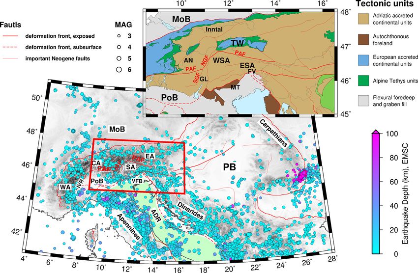
1088                                 A. Jozi Najafabadi et al.: Relocation of earthquakes in the southern and eastern Alps

   The dense temporary seismic SWATH-D network was de-            ing velocity model, starting locations of earthquakes), and
ployed from 2017 to 2019 in the southern and central Alps         the inversion results are data-driven. Moreover, the results
(Heit et al., 2017, 2021) with a total number of 161 stations.    can be statistically analyzed, and thus errors and ambiguities
Given the average station spacing of only 15 km, this network     can be estimated. The method extends the probabilistic relo-
was designed to capture the shallow crustal seismicity (es-       cation approaches (Lomax et al., 2000) by inverting for a set
pecially the depths of the earthquakes) with higher precision     of velocity models well explaining the data.
than the coarser permanent networks, including the AlpArray
network (AASN, with 52 km station spacing; Hetényi et al.,
2018), and to obtain an increased spatial resolution of im-       2   Tectonic setting and local seismicity
ages (e.g., local earthquake tomography, receiver functions),
                                                                  The study region (Fig. 1) is part of the collisional zone be-
even in a region with low or moderate local seismicity. The
                                                                  tween the Adriatic and European tectonic plates. The con-
SWATH-D network is located in a key part of the Adriatic
                                                                  vergence of these plates began no later than 84 Ma, with the
indenter, for which a switch in subduction polarity was pro-
                                                                  onset of collision at ca. 35 Ma (Dewey et al., 1973; Schmid
posed at the transition from the central to eastern Alps (e.g.,
                                                                  et al., 2004; Handy et al., 2010) and culminating since ca.
Lippitsch et al., 2003).
                                                                  24 Ma with north-northwestward indentation of the Adriatic
   In this study, we use a subset of 335 local earthquakes
                                                                  continental lithosphere (Handy et al., 2015). Indentation is
recorded by the SWATH-D network and complemented by
                                                                  still ongoing today (Cheloni et al., 2014; Aldersons, 2004;
a selection of 112 AlpArray network stations nearby to pre-
                                                                  Serpelloni et al., 2016; Sánchez et al., 2018).
cisely relocate the hypocenters of the local earthquakes. The
                                                                     Deformation in the target area (red box in Fig. 1) occurred
dense, high-quality travel time picks created in this study po-
                                                                  within a corner of the Adriatic indenter, which is delimited
tentially lead to constrained hypocenter solutions with high
                                                                  to the north by the Periadriatic Fault (PAF) and to the west
internal consistency. This will enable us to identify the gen-
                                                                  by the Guidicarie Fault (GF). The PAF is a late orogenic
eral pattern of seismicity on the surface and at depth through-
                                                                  fault active in Oligo–Miocene time, which was sinistrally
out the region and contribute to the understanding of active
                                                                  offset by the GF in Miocene time. Just north of the north-
tectonic processes. A further aim of the study is to derive a
                                                                  western corner of the indenter, where the GF and PAF meet,
high-quality dataset suitable to be used in local earthquake
                                                                  the Tauern Window (TW) exposes remnants of the European
tomography (LET).
                                                                  lower plate at the surface (Scharf et al., 2013; Schmid et al.,
   Although locating earthquakes has been a routine task
                                                                  2013; Favaro et al., 2017; Rosenberg et al., 2018). There-
in seismology for decades, there are several challenges re-
                                                                  fore, shortening and exhumation within the TW are attributed
lated to obtaining a precise location. One of them is the
                                                                  to faulting along the Adriatic indenter (Scharf et al., 2013;
trade-off between the hypocenters and the velocity structure
                                                                  Favaro et al., 2017; Reiter et al., 2018). Counterclockwise ro-
(so-called hypocentre–velocity coupling; Kissling, 1988;
                                                                  tation of the Adriatic plate with respect to the Eurasian plate
Thurber, 1992; Kissling et al., 1994). To yield accurate lo-
                                                                  (Le Breton et al., 2017) is interpreted to have induced seismic
cations (especially depths), either the velocity model should
                                                                  activity in the southern Alps (Anderson and Jackson, 1987;
be well known in advance or, particularly in the case of
                                                                  Mantovani et al., 1996; Bressan et al., 2016).
earthquakes occurring within a network (local earthquakes),
                                                                     The thrust front in the eastern southern Alps (ESA) ac-
it has to be simultaneously inverted for (Kissling, 1988;
                                                                  commodates most of the Adria–Eurasia convergence with
Kissling et al., 1994; Thurber, 1983; Husen et al., 1999).
                                                                  pronounced N-oriented present-day motion (Serpelloni et al.,
This is conventionally being done by employing iterative
                                                                  2016; Sánchez et al., 2018). A N-oriented horizontal defor-
inversion strategies based on damped least squares. These
                                                                  mation of ∼2 mm a−1 is observed in the ESA front (northern
methods are quite robust and have been successfully ap-
                                                                  part of the Venetian-Friuli Basin; Sánchez et al., 2018; Mé-
plied for years. However, because they use a linearization and
                                                                  tois et al., 2015; Cheloni et al., 2014) with highest recorded
the damped least-squares approach, they depend not only on
                                                                  geodetic strain rate along the Venetian Front (within the
proper choices of initial values for hypocenter coordinates
                                                                  Montello region, around 45.8◦ N, 12.25◦ E) (Serpelloni et al.,
(close enough to the true location) and the velocity model(s)
                                                                  2016; Verwater et al., 2021). From the Venetian part of ESA
but also on model parametrization (i.e., layers) or regular-
                                                                  toward the Po Basin (PoB), the motion vectors have a slight
ization (i.e., damping factors), which all have to be carefully
                                                                  westward rotation with decreasing magnitudes. In contrast, a
checked and selected.
                                                                  progressive eastward rotation of motion vectors is observed
   Recently, a transdimensional, hierarchical Bayesian ap-
                                                                  from the Venetian area toward the Pannonian Basin. The en-
proach utilizing a Markov chain Monte Carlo (McMC) al-
                                                                  tire Alpine chain is still undergoing uplift, with a maximum
gorithm was implemented for simultaneous inversion of
                                                                  in the inner Alps, e.g., along the border between Switzer-
hypocenters, 1-D velocity structure, and station corrections,
                                                                  land, Austria, and Italy (near 46.6◦ N, 11◦ E) with values of
specifically for the local earthquake case (Ryberg and Haber-
                                                                  ≥ 2 mm a−1 , whereas uplift rates decrease toward the fore-
land, 2019). This approach has the advantage of being largely
                                                                  land (Sánchez et al., 2018).
independent of prior knowledge of model parameters (start-

Solid Earth, 12, 1087–1109, 2021                                                     https://doi.org/10.5194/se-12-1087-2021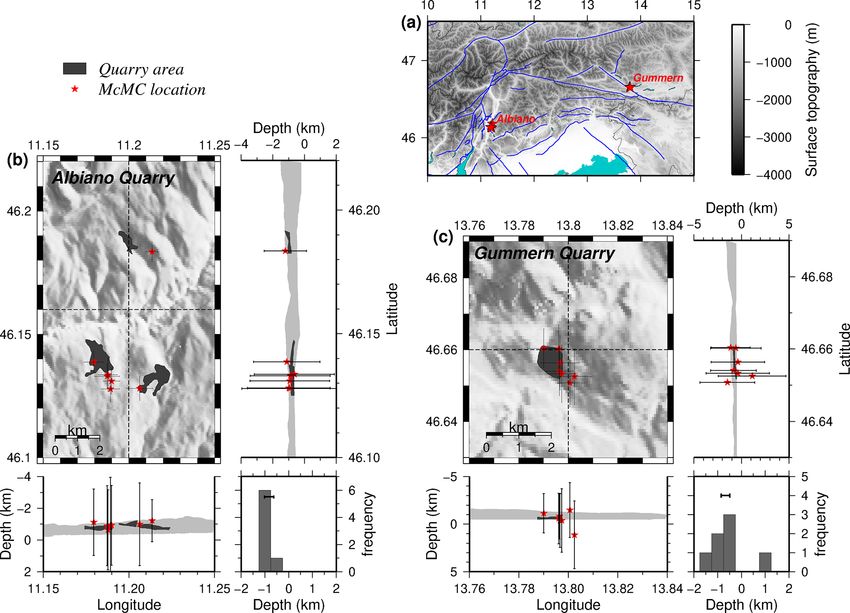
A. Jozi Najafabadi et al.: Relocation of earthquakes in the southern and eastern Alps                                      1089

   Two sedimentary basins, the Molasse and the Po basins          2017, and the network ran for almost 2 years (Heit et al.,
(MoB and PoB in Fig. 1) dominate the shallow structure at         2017, 2021). The network consisted of 151 broadband
the northern and southern borders of the target area. The         seismometers with an average inter-station spacing of
MoB, running along the northern front of the Alps, thick-         15 km. A total of 78 stations equipped with Güralp-3ESPC
ens going across strike from the exposed Variscan base-           seismometers       (https://www.guralp.com/products/surface,
ment (0 km) to the Alpine Front (5 km; see, e.g., depth-to-       last access: 1 November 2020) and Earth Data EDR-210
basement contours in the map of Bigi et al., 1989). The Qua-      recorders (http://www.earthdata.co.uk/edr-210.html, last
ternary and Tertiary sediments of the PoB thicken from 0 km       access: 1 November 2020) transmitted data in near real-time
at its northern margin to about 6 km in the south below the       via the cellular network (online). The other 73 stations,
Apenninic front (Bigi et al., 1989; Waldhauser et al., 2002).     with data accessed during station services (offline), were
   The seismicity in the study area and surrounding regions       equipped with two different kinds of seismometers and
has been monitored routinely for many years with stations         digitizers: 58 of them with Nanometrics portable Tril-
operated by different national and regional networks ( Na-        lium Compact seismometers (https://www.nanometrics.
tional Institute of Geophysics and Volcanology, INGV, and         ca/products/seismometers/trillium-compact, last access:
National Institute of Oceanography and Experimental Geo-          1 November 2020) and CUBE recorders (https://www.
physics, OGS, in Italy; Central Institution for Meteorology       gfz-potsdam.de/en/section/geophysical-deep-sounding/
and Geodynamics in Austria, ZAMG; and Swiss Seismo-               infrastructure/geophysical-instrument-pool-potsdam-gipp/
logical Service in Switzerland, SED). Besides routine cata-       pool-components/seismic-pool/recorder-dss-cube3/,         last
logs, the seismicity has also been investigated in a few seis-    access: 1 November 2020), and the rest with Güralp-
mological studies through various time periods and regions        3ESPC seismometers and Earth Data PR6-24 recorders
(Blundell et al., 1992; Solarino et al., 1997; Galadini et al.,   (http://www.earthdata.co.uk/pr6-24.html,       last    access:
2005; Diehl, 2008; Viganò et al., 2013; Reiter et al., 2018,      1 November 2020). In Autumn 2018, the network was
among others). Diehl (2008) compiled the local earthquake         complemented with an additional 10 online stations in the
data from 14 seismic networks in the greater Alpine region        northeastern edge by LMU-Munich. All SWATH-D seismic
from 1996 to 2007 and created a uniform and consistent relo-      stations recorded the data continuously at 100 samples per
cated event catalog. The SHARE European Earthquake Cat-           second (sps).
alog (Grünthal et al., 2013) comprised homogeneous earth-            In order to enlarge the azimuthal coverage for earthquakes
quakes from 1000 to 2006.                                         occurring in the periphery of the SWATH-D framework, we
   These studies indicate that seismic activity is clustered in   additionally selected 112 stations of the larger-scale AlpAr-
the Friuli-Venetia (FV), Giudicarie–Lessini (GL), and the In-     ray Seismic Network (AASN; Hetényi et al., 2018) to include
ntal regions (Fig. 1). The FV region is located along the         their waveform data in the analysis.
thrust-and-fold belt marking the active Adria–Europe plate
boundary and was struck by several earthquakes of MW ≥ 6
                                                                  3.2   Seismic events, arrival time picks, and phase-type
over the last several centuries (Slejko, 2018). The energy was
                                                                        identification
released on a system of E–W south-verging thrusts (some of
which are blind or unknown), as well as on backthrusts and
oblique-slip faults (Nussbaum, 2000; Galadini et al., 2005;       The national seismological agencies of Italy (INGV and
Slejko, 2018; Romano et al., 2019). The GL region is located      OGS), Austria (ZAMG), and Switzerland (SED) provide
in the deformation zone along the western margin of Adriatic      comprehensive earthquake catalogs (minimum magnitude
indentation with two major fault and fold systems charac-         −0.8 by ZAMG) in our study region. Therefore, the process
terized by high seismic activity: the Giudicarie Belt and the     of event detection was skipped and an integrated event list
Schio-Vicenza strike-slip fault (Viganò et al., 2015). In con-    from the national agencies, after removal of common events,
trast, the area east of the northern Guidicarie Fault (NGF) has   formed a proper list of 2639 local events (see Appendix A
obviously been much less active since at least 1994 (Viganò       for more information) for arrival time picking. Considering
et al., 2015).                                                    this large number of events and 273 selected permanent and
                                                                  temporary stations, we applied a modified version of the au-
                                                                  tomated multi-stage workflow from Sippl et al. (2013) to
3     Data acquisition and processing                             the waveform data for picking the arrival times of P and S
                                                                  waves. This workflow was originally implemented for pro-
3.1    Network data                                               ducing a complete catalog of well-located earthquakes and
                                                                  reliable arrival times using continuous passive seismic data in
For this study, we used mainly data of the SWATH-D                the Pamir–Hindu Kush region (Sippl et al., 2013). We, subse-
network, which was temporarily deployed in a roughly              quently, assessed the performance of the picking algorithms
rectangular region in northern Italy and southeastern Austria     by quality-checking of time and phase-type uncertainties of
(black box in Fig. 2). The installation started in Summer         the picks (Appendix B).

https://doi.org/10.5194/se-12-1087-2021                                                     Solid Earth, 12, 1087–1109, 2021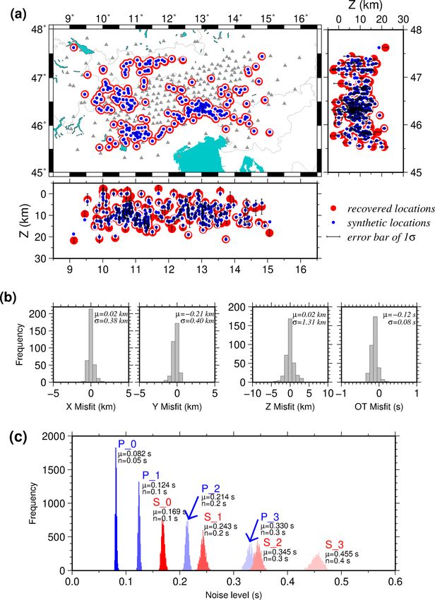
1090 A. Jozi Najafabadi et al.: Relocation of earthquakes in the southern and eastern Alps
Figure 1. Geological map of the Alps showing major deformation fronts, faults, geographical subdivisions, tectonic units, and seismicity
(seismic events between January 2000 and December 2012 with a magnitude larger than 3 from the European-Mediterranean Seismological
Centre). The light green zone indicates the outline of the Adriatic plate. The tectonic units of the study area (red box) are shown on the
upper-right inset map. The maps are modified from Handy et al. (2010) and Schmid et al. (2004, 2008). Abbreviations are as follows: WA
stands for western Alps, CA stands for central Alps, SA stands for southern Alps, EA stands for eastern Alps, ADR stands for Adriatic plate,
IVR stands for Ivrea body, PB stands for Pannonian Basin, VFB stands for Venetian-Friuli Basin, PoB stands for Po Basin, MoB stands for
Molasse Basin, TW stands for Tauern Window, PAF stands for Periadriatic Fault, NGF stands for northern Giudicarie Fault, SGF stands for
southern Giudicarie Fault, ESA stands for eastern southern Alps, WSA stands for western southern Alps, MT stands for Montello, GL stands
for Giudicarie–Lessini region, FV stands for Friuli-Venetia region, and AN stands for Austroalpine nappes.
selected events with azimuthal gap less than 200◦ and root
mean square (rms) less than 1 s, which resulted in 384 event
(18 390 P and 7762 S picks). This visual (manual) inspection
of this dataset was carried out by removing or modifying ob-
vious mispicks (mainly at large epicentral distances) and also
re-picking the missed arrivals (mostly S picks at small epi-
central distances).
This manual (visual) inspection was mainly performed on
individual station data. The direct Pg (Sg), Moho-reflected
PmP (SmS), and Moho-refracted Pn (Sn) phases arrive
closely spaced in time, especially in the triplication zone,
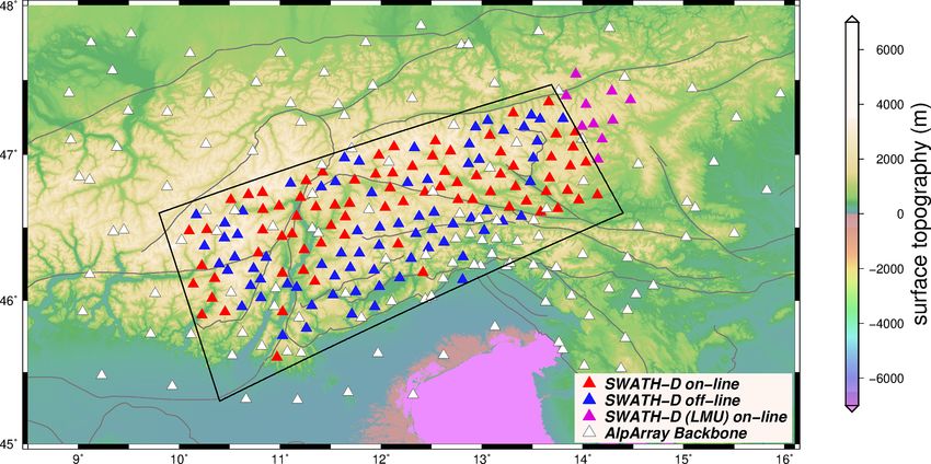
Figure 2. Distribution of seismic stations of the SWATH-D network potentially leading to phase-type misidentification. The PmP
(red, blue, purple) and selected stations of the AASN (white). The (SmS) is always a secondary arrival, but its amplitude can
black box indicates the periphery of the SWATH-D network. The dominate the first arrival and thus be easily mispicked. On
faults are from Schmid et al. (2004, 2008) and Handy et al. (2010). the other hand, for epicentral distances larger than the tripli-
cation zone, the Pn (Sn) amplitude can be so weak that the Pg
(Sg) or PmP (SmS) be wrongly identified as the first arrival.
As described in Sect. B2, the number of mispicks and In the local earthquake case, and particularly for regions with
picks ignored by the automatic procedure was quite large. varying Moho topography and significant lateral variations in
Therefore, a dataset with relatively highly constrained events the crustal structure, something to be expected for the Alps,
was selected for visual (manual) inspection. Since the num- the phase-type identification is even more challenging (Diehl
ber of picks in this stage (after the automatic procedure) is et al., 2009b). Since the inversion is based on the first ar-
not the most reliable information on the location precision rival times we looked at the waveforms in epicentral distance
(see Sect. B2) and also considering that this data is aimed plots for larger events for which we expect the later phases,
for high location accuracy of the occurring earthquakes, we inspected the picks, and corrected or adjusted where needed.
Solid Earth, 12, 1087–1109, 2021 https://doi.org/10.5194/se-12-1087-2021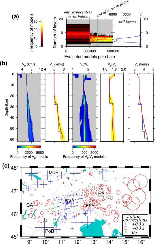
A. Jozi Najafabadi et al.: Relocation of earthquakes in the southern and eastern Alps                                                  1091

                                                                          Figure 4. Histograms of high-quality P and S picks per event for
                                                                          301 well-constrained local earthquakes used for simultaneous inver-
                                                                          sion of hypocenters, 1-D velocity models, and station corrections.
Figure 3. Modified Wadati diagram based on P and S picks after
visual (manual) analysis (the color indicates number of picks; please
see the color palette table on the right). The origin times (t0 ) of
the earthquakes are provided by the single-event localization using       The average number of picks per event is 32 for P and 18 for
HYPO71 hypocenter determination program (Lee and Lahr, 1975).             S, with maximum of 157 and 118, respectively (Fig. 4).
The solid black line shows the fit to the data by linear least squares,      In order to investigate the seismicity pattern, we use the
and its slope indicates the VP /VS ratio of 1.72. The dashed lines        travel time data of an additional 43 local earthquakes with
show values with ts − tp = 0.72tp ± 3 s.                                  slightly fewer picks (minimum of eight P picks and two S
                                                                          picks) to the main dataset and relocate them using the VP ,
                                                                          VP /VS , station corrections, and noise levels from the simul-
                                                                          taneous inversion (Sect. 6.3). This updated dataset contains
                                                                          344 earthquakes, 12 420 P picks, and 7192 S picks.
However, we would like to point out that even with these pro-
cedures we cannot rule out a certain amount of misidentified
phases.                                                                   4     Method
   An inspection for identifying potential quarry blasts (and
other anthropogenic sources) was simultaneously performed                 4.1    Probabilistic Bayesian inversion
during the visual inspection. Criteria for potential quarry
blasts were (1) relatively small number of S-picks, (2) rel-              Considering that hypocenter locations and velocity model are
atively small S/P amplitude ratios (see, e.g., Walter et al.,             inherently linked to each other (coupled hypocenter-velocity
2018), and (3) large surface waves (observed dispersive                   problem, e.g., Kissling, 1988; Thurber, 1992; Kissling et al.,
waveform characteristics). Based on our assessment, we clas-              1994), especially in the local earthquake case, a simultane-
sified the events into 344 earthquakes, 15 potential blasts, and          ous inversion for hypocenters and velocity structure (and/or
25 unclear events.                                                        station corrections) is needed. In this study, different to the
   A Wadati diagram (Wadati, 1933; Kisslinger and Eng-                    conventional approach of damped least squares, we use a
dahl, 1973; Diehl, 2008) was used to calculate the VP /VS                 Bayesian approach (Bayes, 1763). Bayesian approaches have
ratio of the earthquakes, which is 1.72 (calculated by lin-               been applied in a number of geophysical studies (Tarantola
ear least squares; Fig. 3). Furthermore, S picks with S–P                 et al., 1982; Duijndam, 1988a, b; Mosegaard and Tarantola,
travel time differences larger than 4 s off the main trend were           1995; Gallagher et al., 2009; Bodin et al., 2012a, b; Ry-
removed (however, this was only 0.3 % of all picks). Af-                  berg and Haberland, 2018). Ryberg and Haberland (2019) re-
ter this removal, only 2 % of the whole observations have                 cently implemented a hierarchical, transdimensional Markov
ts − tp > 0.72tp ± 3 s. We notice that at P travel times larger           chain Monte Carlo (McMC) approach for the joint inversion
than ∼ 25 s the observations tend to slightly larger S–P travel           of hypocenters, 1-D velocity structure, and station correc-
time differences, potentially indicating a higher VP /VS ratio            tions for the local earthquake case. While with classical in-
at larger depth, i.e., in the upper mantle.                               version techniques a discrete best-fitting model m (i.e., lo-
   For the simultaneous inversion of hypocenters, 1-D veloc-              cations, velocity model, etc.) is derived, in the Bayesian in-
ity models, and station corrections, we used the events with              ference all the parameters of the model m are represented
at least 10 P picks and 5 S picks and an azimuthal gap less               probabilistically. For the theoretical background the reader
than 180◦ , which comprises 301 local earthquakes. The ar-                is referred to Bodin and Sambridge (2009) and Bodin et al.
rival time dataset consists of 11 084 P picks and 6496 S picks            (2012a, b). We define a uniform and wide range of values
(quality classes of 0 to 3) with average picking errors of 0.12           for each individual model parameter (before knowing the ob-
and 0.21 s for P and S observations, respectively (Table 1).              served data; prior) and after performing the inversion for ran-

https://doi.org/10.5194/se-12-1087-2021                                                               Solid Earth, 12, 1087–1109, 2021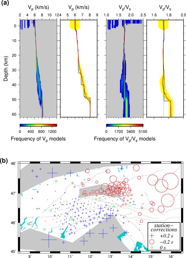
1092                                              A. Jozi Najafabadi et al.: Relocation of earthquakes in the southern and eastern Alps

Table 1. Statistical parameters of high-quality P and S pick dataset of 301 well-constrained local earthquakes used for simultaneous inversion
of hypocenters, 1-D velocity model, and station corrections.

                                Quality class                           P picking       Number         S picking       Number
                                                                    uncertainty (s)   of P-picks   uncertainty (s)   of S-picks
                                0                                             ±0.05       4170              ±0.1          2715
                                1                                              ±0.1       3462              ±0.2          1254
                                2                                              ±0.2       2327              ±0.3          1563
                                3                                              ±0.3       1125              ±0.4           964
                                Sum (no.)                                                11 084                           6496
                                Average picking error (s)                                  0.12                            0.21

dom combinations of the parameters, we derive a probabil-                             solver (Podvin and Lecomte, 1991) for the forward calcula-
ity distribution individually for each model parameter (af-                           tion. This algorithm requires a regular mesh. Therefore, the
ter combining the prior information with the observed data;                           irregular velocity model is converted to a fine and uniform
posterior). Thus, a large suite of models is generated, all of                        mesh by setting the velocity at each mesh point to the value
them fitting the travel time observations. The choice of a uni-                       of the nearest point from the irregular model (VPi or VP /VSi ).
form and extensively wide range of model parameters (Ta-                              The fine mesh used by the Eikonal solver has a cell spacing
ble 2) guarantees that the final model is dominated by the                            of 1 km vertically and horizontally.
data rather than by the prior information (i.e., starting model,                         Once the travel times are calculated, a misfit function, par-
choice of parameters).                                                                ticularly for each model, is defined as the summed squared
                                                                                      differences between the observed (d) and calculated travel
4.2    Model parametrization and forward problem                                      times. The misfit function is then used to build the Gaussian
                                                                                      likelihood function and the posterior values of the proposed
Hypocenters are described by spatial (x0 ,y0 ,z0 ) and temporal                       model (for detailed information one could refer to Ryberg
(t0 ) coordinates and the 1-D velocity structure is described by                      and Haberland, 2019).
a variable number of horizontal layers with individual values
of VP and VP /VS . Moreover, the model m comprises station                            4.3   Markov chain Monte Carlo (McMC) algorithm
corrections for P and S waves (τ P and τ S ), which account for
travel time effects (delayed or earlier arrivals) due to devia-                       Given the Bayesian approach described above, the McMC
tions of the 1-D model from the real 3-D velocity structure                           algorithm generates an ensemble of models with parameters
in the shallow subsurface beneath the stations. The inversion                         within the prior distribution. We mainly follow the hierar-
also derives the quality of the data expressed as noise levels                        chical, transdimensional procedure proposed by Ryberg and
for P and S picks (σP and σS ), which are also unknowns in                            Haberland (2018, 2019) that supports the calculation of both
the inversion. The noise includes actual picking errors, sys-                         model parameters and model dimensionality. The evolution
tematic errors of observations or measurements, and any ap-                           of a model along the Markov chain consists of four main
proximation or errors of forward travel time calculation (see                         steps: (1) choose a random initial model m (Table 2). (2)
below) and is assumed to be normally distributed and uncor-                           Generate a new model from the prior distribution by per-
related. Therefore, the complete model to be inverted for is                          turbing the current model parameters (changing one of the
defined as follows:                                                                   velocity parameters of a random node, shifting the position
m = [K, VPi , VP /VSi , hi , xj , yj , zj , tj , τ P k , τ S k , σP , σS ],    (1)    of a random earthquake, adding a new layer, removing a ran-
                                                                                      dom layer, altering one of the noise parameters, changing a
where K is the number of layers; h is layer depth; and i,                             randomly selected station correction. The changes in the VP ,
j , and k refer to layer, earthquake, and station index, re-                          VP /VS , cell position (i.e., layer), and noise levels must be ac-
spectively. It should be noted that the number of layers is                           cording to Gaussian probability distribution centered at the
also unknown. In other words, the model space dimension is                            current value. The values of the new model are randomly se-
not fixed in advance and hence the posterior is a transdimen-                         lected within very wide bounds (Table 2) and thus do not
sional function.                                                                      truncate the posterior probability distribution. (3) The for-
   In order to sample models from the prior probability dis-                          ward calculation (Sect. 4.2) is then performed on the new
tribution, we apply McMC approach to create a huge number                             model. The newly estimated travel time data are compared
of different models m by random selection of model parame-                            with the observed data d and then the misfit function, data
ters (see Eq. 1 and Sect. 4.3). Accordingly, to compute travel                        likelihood, and the posterior probability are determined. (4)
times the forward problem has to be solved a very large num-                          The newly proposed model is accepted or rejected based on
ber of times. We use the 2-D finite differences (FD) Eikonal                          the criteria of Bodin and Sambridge (2009). If the new model

Solid Earth, 12, 1087–1109, 2021                                                                          https://doi.org/10.5194/se-12-1087-2021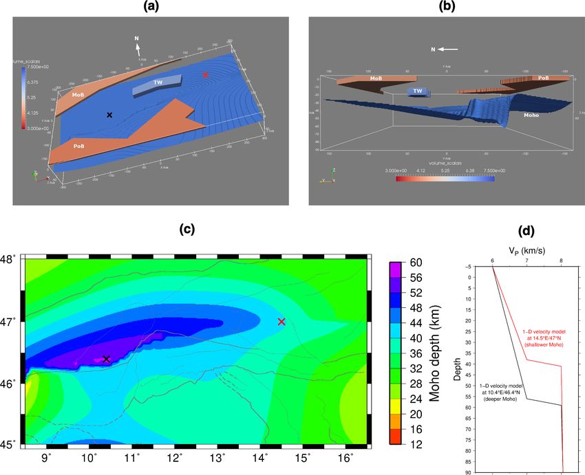
A. Jozi Najafabadi et al.: Relocation of earthquakes in the southern and eastern Alps                                                1093

Table 2. Prior distribution (model space), starting model, and width of Gaussian distribution for each model parameter.

    Model parameter                  Lower boundary   Upper boundary      Starting model                                  Gaussian
                                                                                                                          Width
    Earthquake epicenter (x, y)      −300 km          +300 km             random and uniform                              2 km
    Earthquake depth (z)             0 km             200 km              random and uniform                              2 km
    VP                               2 km s−1         12 km s−1                              6 and sigma = 0.5 km s−1
                                                                          normal with mean = √                            0.05 km s−1
    V P /V S                         1                2.5                 normal with mean = 3 and sigma = 0.2            0.05
    Layer depth (h)                  1                200                 random and uniform                              10 km
    Number of layers                 1                200                 Normal with mean = 5 and sigma = 3              –
    Noise σP and σS                  0.001 s          10 s                1s                                              0.01 s
    Station correction τ P and τ S   −5 s             5s                  0s                                              0.05 s

is rejected, then the current or old model is retained by reit-         and finally inverted them in the same way as the real data
erating step 2. However, there is still a probability of accep-         (see below). Comparing input event locations (synthetic) and
tance even if the fit of the new model is worse than that of            the inverted (output) ones allows us to study the recovery of
the old model. If the model is accepted (i.e., when it is better        the hypocenters, location consistency, and potential system-
than the previous model) then it acts as a starting model for           atic errors related to the use of a 1-D model, which we can
another iteration (step 1).                                             generally expect for the derived real hypocenters. For exam-
   By reiteration of steps 1 to 4, a chain of models is pro-            ple, it can be studied whether events at the periphery or in
duced, which is in fact the Markov chain. This chain is                 certain parts of the model have systematically larger uncer-
continued until the misfit is no longer significantly decreas-          tainties (e.g., due to their location and/or spatial distribution
ing (burn-in phase). Thereafter, a stationary model space               of picks). Furthermore, we can study how the (output) 1-D
sampling is achieved. If these sequences are repeated long              model looks in comparison to the (input) 3-D model, how
enough, a chain provides an approximation of the poste-                 large the derived noise is in relation to the synthetic input
rior distribution for the model parameters. To accelerate the           noise, and how the pattern of station corrections corresponds
model space sampling, up to 1000 separate and independent               to the shallow velocity anomalies. Similar tests are standard
chains are investigated in parallel.                                    in structural studies (i.e., LET) to study the recovery of cer-
   The main idea of the McMC method is to keep prior as-                tain features.
sumptions of the model parameters (conventionally used as                  In our synthetic 3-D background model, the course of the
initial values) at a minimum and thus minimize unwanted                 crust–mantle boundary is inspired by the Moho topography
artificial effects on the final model. Therefore, the McMC              of the European and Adriatic plates from Spada et al. (2013);
method only uses the travel times and does not directly de-             however, we adopted it in a simplified way without features
pend on initial hypocenters, origin times, velocity models,             such as crustal stacks (overlapping Mohos of the two in-
or even the model parametrization (e.g., grid node spacing).            volved plates) or the proposed Moho hole. Our main aim
Nevertheless, the selection of picks in the (semi-automatic)            of this simplified adaption is studying the influence of a 1-
picking procedure involves the comparison of the observed               D model class on the derived hypocenters after the inversion
travel times with those based on preliminary hypocenters                and the goal is not recovering the exact velocity structure. We
(which depend on initial velocity models). Therefore, the re-           assigned typical crustal velocities to the upper layer, start-
sults of the inversion can sensu stricto depend to some degree          ing with 6 km s−1 and increasing to 7 km s−1 at the base of
on initial values.                                                      this crustal layer. Thereafter, the velocity increases from 7 to
                                                                        8 km s−1 within a thin zone of 3 km with a strong gradient.
                                                                        Following this, the velocity increases again gradually until
5    Uncertainty estimates using synthetic tests                        it reaches 8.05 km s−1 at 90 km depth (Kennett et al., 1995;
                                                                        Christensen and Mooney, 1995). The Moho depth in the tar-
As a variable Moho topography and complex lithosphere                   get area changes from 22 km along the flank of the Ivrea body
structure are expected for our study region, the 1-D model              to more than 55 km along the Adria–Europe plate boundary
derived by and used in our inversion can only be a rough ab-            (Spada et al., 2013). We considered the model’s surface to be
straction of the real conditions. Nevertheless, this simplifica-        −5 km to avoid wave propagation through the air.
tion could potentially have influence on earthquake location               In order to simulate realistic 3-D effects in the context of
correctness and accuracy. To assess the performance of our              expected crustal structure, we superimposed shallow high-
inversion strategy in this respect, using a 3-D velocity model          and low-velocity anomalies onto the background 3-D model
and earthquake and station distribution of the real data, we            presented above. We assumed that the hard rocks of the Eu-
calculated the synthetic travel times, added synthetic noise

https://doi.org/10.5194/se-12-1087-2021                                                              Solid Earth, 12, 1087–1109, 2021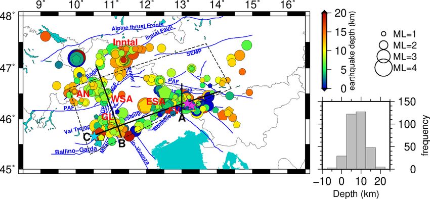
1094                                  A. Jozi Najafabadi et al.: Relocation of earthquakes in the southern and eastern Alps

ropean basement exhumed in the TW have higher veloci-               ters is quite close to zero with uncertainties of ∼ 400 m in
ties than the surrounding Austroalpine nappes and thus form         epicenter, 1.31 km in depth, and 0.12 s in origin time. Never-
a high-velocity anomaly (+5 %) within a rough outline of            theless, we note that although the epicenters of most of the
the TW and from the surface to the depth of 10 km (for              earthquakes throughout the study area are recovered well, the
more information on the TW, see, e.g., Bertrand et al., 2015).      depths of the events at the edges of the network are less well
Furthermore, we designed lower-velocity anomalies for the           recovered and that their uncertainties are also systematically
PoB and MoB sedimentary basins (the coarse outlines of the          larger (see Fig. 6). The recovered noise levels, which are rep-
basins are taken from Waldhauser et al., 2002). An average          resentative of the unresolved part of the travel times, are cal-
VP of 4.35 km s−1 is considered for the entire MoB from the         culated for individual pick types and quality classes sepa-
model’s surface down to 2 km depth. For the PoB, a layer of         rately (Fig. 6c). They are close to the random noise, which
6 km thickness starting from the model’s surface and with VP        was added to the synthetic arrival times (manual arrival time
of 2 km s−1 less than the background model is constructed.          uncertainties in Table B2); however, they are slightly higher.
The shallow anomalies are then inserted in the background           This deviation could be explained by the forward modeling
model. Taking the shallow anomalies into account not only           errors and the fact that the inversion derives a 1-D velocity
makes the model more realistic but also allows us to check          model from data of a 3-D input model.
whether the station corrections reflect travel time deviations         Figure 7a shows the derived VP and VP /VS models as heat
due to velocity variations in the shallow subsurface. Figure 5      maps (posterior distribution of all the models). In addition,
displays the 3-D synthetic VP model from different views and        it shows the average value (red line), standard deviation of
also the 1-D model at two different√ viewpoints. The VP /VS         all the inferred models (yellow zone), and a reference model
ratio in the entire model is set to 3.                              with maximum likelihood (blue line), i.e., maximum poste-
   The P and S arrival times are calculated using the 3-D           rior probability (similar to Ryberg and Haberland, 2019). As
FD Eikonal solver (Podvin and Lecomte, 1991; Tryggva-               seen, no clear single Moho velocity jump is recovered, but it
son and Bergman, 2006). We generated an FD grid with                is modeled by a gradual increase of the velocities at depths
an increment of 1 km horizontally and vertically, resulting         from 30 to 50 km. We attribute this to the variable Moho
in a grid dimension of 601 × 321 × 96 with a total number           topography, which cannot be modeled by the 1-D velocity
of 18 520 416 nodes. For simulating a realistic travel time         model per se, and potentially lower resolution due to less ray
dataset, we adopted the geometry of stations and hypocenters        coverage in this depth range. Because of a dense ray coverage
of the real data. Using 344 earthquakes, in total 12 534 P and      from the surface down to a depth of ∼ 20 km, the V P uncer-
7258 S synthetic picks resulted from the forward calculation.       tainty is almost zero in this depth range. In the depth inter-
Thereafter, according to the manual arrival time uncertainties      val with strong Moho topography, the uncertainty varies be-
in Table B2, we added random noise (0.05, 0.1, 0.2, 0.3, 0.1,       tween 0.1 and 0.66 km s− 1. The uncertainty values are com-
0.2, 0.3, and 0.4 for P-0, P-1, P-2, P-3, S-0, S-1, S-2, and S-     patible with the standard deviation of the lateral heterogene-
3, respectively) to the arrival times, and this dataset was then    ity in the synthetic 3-D velocity model (∼ 0.8 km s− 1 above
used for the simultaneous inversion by McMC.                        2 km, ∼ 0.05 km s− 1 between 2 and 20 km, and between 0.1
   To explore the model parameters, 100 Markov chains each          and 0.5 km s− 1 below 20 km depth). Thus, we think that the
with 1000 random initial models are used for simultaneous           increased standard deviations beneath ∼ 30 km depth indi-
inversion of McMC. Following the strategy in Ryberg and             cating reduced and fading resolution are due to both variable
Haberland (2019), we derived ∼ 15 000 of the final mod-             Moho topography and reduced ray coverage; however, their
els from the Markov chains (more information is given in            exact contribution is hard to discern.
Sect. 6) to define model parameters based on the average µ             The VP /VS ratio was fixed to the square root of 3 for the
and standard deviation σ . For the earthquake epicenters (x         whole region in the forward modeling, and the same value
and y) and station corrections (τ P and τ S ) the classical aver-   is recovered down to ∼ 35 km depth with almost zero uncer-
age of the Gaussian distribution is used. However, the depth        tainty (less than 0.02). The uncertainty of VP /VS increases
distribution of shallow earthquakes is truncated by the up-         below 35 km depth to a maximum value of 0.046, indicating
per model boundary. In order to accommodate this, we used           that this deeper part of the model is not well resolved.
an algorithm based on truncated Gaussian distributions (Ry-            The station corrections (Fig. 7b) correspond to a large ex-
berg and Haberland, 2019) to derive true depth averages and         tent to the shallow anomalies of the 3-D synthetic model
uncertainties. The VP and VP /VS values are defined based           (Fig. 5). The shallow high-velocity anomaly in the TW is ex-
on the modified average (Ryberg and Haberland, 2018) and            pressed by negative corrections (large circles) corresponding
standard deviation.                                                 to earlier arrivals, while the shallow low-velocity anomalies
   Figure 6 represents the recovery of the earthquakes. Fig-        of the PoB and MoB correspond to positive corrections (large
ure 6a shows that the epicenters are recovered very well (the       crosses) reflecting later arrivals.
blue dots are located on top of red circles). Further assess-
ment of the earthquake recovery (Fig. 6b) demonstrates that
the average misfit between synthetic and recovered hypocen-

Solid Earth, 12, 1087–1109, 2021                                                       https://doi.org/10.5194/se-12-1087-2021
A. Jozi Najafabadi et al.: Relocation of earthquakes in the southern and eastern Alps                                               1095

                                                                                √
Figure 5. The 3-D synthetic VP velocity model. The VP /VS ratio was fixed to 3 in the entire model. (a) and (b) Contours of the Moho and
shallow anomalies of the PoB, MoB, and TW from different view directions. (c) Modified Moho depth map based on Spada et al. (2013).
(d) A 1-D velocity model of two different locations with shallower and deeper Moho retrieved from the 3-D synthetic velocity model (the
locations are shown with red and black crosses in (a) and (c), respectively). The faults are the same as those in Fig. 2.

6   Results and discussion                                            ity. The final models have stationary rms misfits of 0.36 s
                                                                      (Fig. 8).

                                                                      6.1   The 1-D velocity model and station corrections
For the simultaneous inversion of the hypocenters, the 1-D
velocity model, and the station corrections, we used the travel       It turns out that the algorithm needs roughly five layers to
time dataset of the earthquakes (Sect. 3.2). In the simulta-          best fit the data (Fig. 9a). Similar to the synthetic test (Fig. 7),
neous inversion, for the first 300 000 models of the Markov           the final velocity models are shown with the average of
chains, only the hypocenters are allowed to be changed.               all remaining models and the model with maximum poste-
Thereafter, VP , VP /VS ratio, station corrections, and noise         rior probability. In general, for both VP and VP /VS models
levels additionally are permitted to change, adding 300 000           (Fig. 9b) the average value (red line) varies gently, whereas
more models to the Markov chain. After inversion of 400 000           the model with maximum posterior probability (blue line) is
models in each Markov chain, the model space reached the              rather coarse and contains discontinuities.
stationarity (end of burn-in) phase. Thereafter, badly con-              The derived VP model starts with a rather high value of
verging chains are automatically excluded, and every 1000th           5.94 km s−1 at the surface and increases only very gently
model is stored from the remaining models after the burn-             down to a depth of around 20 km. After a zone of higher
in phase. The stored models of each chain are combined (in            velocity gradient in the average model around (and a step-
total ∼ 15 000 models) to calculate the posterior probabil-           like increase of the reference model at) ∼28 km depth, ve-

https://doi.org/10.5194/se-12-1087-2021                                                           Solid Earth, 12, 1087–1109, 2021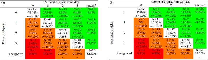
1096                                     A. Jozi Najafabadi et al.: Relocation of earthquakes in the southern and eastern Alps

Figure 6. (a) Recovery of the hypocenters after synthetic test. Red circles are recovered earthquakes with a 1σ error bar (error bars of latitude
and longitude are invisible at this scale), and blue dots are the synthetic locations. The gray triangles show the stations. (b) Histograms of the
misfit between recovered hypocenters and original ones. The hypocenters are recovered very well, with an average misfit of 20 m (±380 m)
in longitude, 210 m (±400 m) in latitude, 110 m (±1.131 km) in depth, and 0.12 s (±0.08 s) in origin time. (c) The recovered noise levels
after McMC for individual pick types and quality classes are slightly higher than the random noise, which was added to the synthetic travel
time data.

locities reach ∼6.8 km s−1 at ca. 30 km (down to ca. 45 km                    Below ca. 45 km depth, velocities increase further up to
depth). Down to this depth the uncertainties (1σ ) indicat-                7.85 km s−1 at 60 km depth; however, standard deviations
ing the resolution increase from 0.01 km s−1 (very good) to                (1σ ) between 0.3 and 0.42 km s−1 indicate only poor reso-
0.28 km s−1 (fair). Our derived VP model in the upper crust –              lution in this depth range. A single step-like increase from
except for the uppermost layer shallower than 3 km – is sim-               “crustal” to “upper mantle” velocities (as at 35 km depth in
ilar to the Diehl et al. (2009b) model, an increase for values             the Diehl et al. (2009b) model) cannot be observed, which
above 6.5 km s−1 is observed deeper than in the latter model.              we attribute either to (1) the expected strong depth variabil-

Solid Earth, 12, 1087–1109, 2021                                                                 https://doi.org/10.5194/se-12-1087-2021
A. Jozi Najafabadi et al.: Relocation of earthquakes in the southern and eastern Alps                                                    1097

                                                                       Figure 8. On the left histogram, the rms misfit along Markov chains
                                                                       during the inversion evolution is shown (color indicates number of
                                                                       models; please see color palette table on the left). Before the red line
                                                                       (300 000 models), only the hypocenters are perturbed and beyond
                                                                       that the VP , VP /VS ratio, station corrections, and noise levels are
                                                                       allowed to change as well. The green line indicates the end of the
                                                                       burn-in phase after ∼ 400 000 models. On the right histogram, the
                                                                       rms misfit for all the models after burn-in phase is shown. The best-
                                                                       fitting models are characterized by an average 0.36 s rms misfit.

                                                                       complex crustal structure, a geologically meaningful inter-
                                                                       pretation of the derived VP model is hardly possible.
                                                                          The VP /VS model starts with high values at the surface
                                                                       (to ∼ 5 km depth) and shows reduced values of around 1.70
                                                                       down to 22 km depth before reaching 1.77 at greater depths
                                                                       (with uncertainty between 0 and 0.02). However, 1σ values
                                                                       of 0.02 to 0.045 indicate only poor resolution at depth larger
Figure 7. (a) Recovery of the VP and VP /VS models after the syn-      than around 30 km, which we associate to only a few Sn ar-
thetic test. The results are shown with heat maps (probability his-    rivals. This was basically expected from the Wadati diagram
togram vs. depth; warm and cold colors correspond to higher and        (Fig. 3) and is in agreement with values previously derived,
lower probabilities, respectively) with gray areas showing zones
                                                                       e.g., by Viganò et al. (2013). Both VP and VP /VS models are
with no model achievement. The modified average model (solid red
line), most probable model (solid blue line), and corresponding un-
                                                                       available in the Supplement S1.
certainty of 1σ (yellow zone) for both                                    The station corrections derived from the McMC simulta-
                                   √ VP and VP /VS models are
shown as well. The VP /VS ratio of 3 is displayed with the dashed      neous inversion potentially indicate local, shallow 3-D veloc-
green line. (b) Recovered P wave station corrections of all the sta-   ity anomalies in the subsurface, which cannot be accounted
tions that were involved in the McMC inversion. Blue crosses show      for by the 1-D model. The McMC inversion assumes that P
positive values reflecting lower velocities, and red circles display   and S station corrections have an average of zero. Negative
negative values indicating higher velocities than expected. Regions    corrections indicate earlier wave arrival and thus higher ve-
indicated in gray have shallow high- or low-velocity anomalies (see    locities in the (shallow) subsurface, whereas positive correc-
Fig. 5 for more information). Symbol size corresponds to correction    tion implies delayed arrival that is indicative of lower veloc-
amplitude. The faults are same as Fig. 2.                              ities.
                                                                          The pattern of corrections (Fig. 9c) shows coherent nega-
                                                                       tive corrections associated with the EA, ESA, and CA. The
                                                                       large negative values in the eastern part (east of 15◦ E) might
ity of the Moho in the study area (see the discussion of the           be related to proximity to the edge of the network and thus be
synthetic model in Sect. 5) and a gradual course of the 1-             dominated by mantle phases (faster arrivals). Surprisingly, in
D model due to lateral averaging in this depth range, (2)              between the negative values in the Alpine Chain, a pattern of
the relatively small number of Pn arrivals, and/or (3) lim-            slight positive corrections in the WSA is observed. Besides,
ited maximum observation distances. Influences by wrongly              extreme positive corrections are seen in the PoB and MoB
picked late-arriving Pg arrivals at large distances (instead of        as expected for sedimentary basins, which is also consistent
Pn phase) cannot totally be ruled out.                                 with the results of the synthetic test (see Sect. 5). A pro-
   As a 1-D model cannot be representative of the 3-D struc-           nounced pattern specifically related to the TW as seen in our
ture, especially in a region with expected irregular Moho and          synthetic test is not observed so clearly in the real data, sug-

https://doi.org/10.5194/se-12-1087-2021                                                              Solid Earth, 12, 1087–1109, 2021
1098 A. Jozi Najafabadi et al.: Relocation of earthquakes in the southern and eastern Alps
gesting a different structure in the shallow subsurface. The
pattern of stations in the ESA and a few stations in the WSA
and CA agree very well with results by Diehl et al. (2009b).
A detailed interpretation of the pattern of the station cor-
rections is highly ambiguous because they contain a superpo-
sition of site effects and/or effects from 3-D structural varia-
tions, as well as a lot of smearing. Nevertheless, the general
concept of simultaneously inverting local earthquake datasets
for a (simplified) 1-D velocity model, hypocenter positions,
and origin times and reactions proved to be very powerful for
accurately localizing earthquakes (see e.g., Kissling, 1988).
Moreover, the general pattern of corrections can indicate the
consistency of phase data.
6.2 Estimation of hypocenter accuracy based on
relocation of quarry blasts
To validate the localization procedure, the detected 15 quarry
blasts (based on visual inspections; see Sect. 3.2) were inde-
pendently relocated by McMC using the previously derived
1-D velocity model and station corrections from the simul-
taneous inversion (Sect. 6.1). Figure 10 focuses on the blast
distribution associated with two quarry areas close to the vil-
lages of Albiano (Italy) and Gummern (Villach, Austria). Af-
ter the relocation of the blasts, we see that the epicenters are
located within the quarry areas and that the depths are in the
range of the quarry topography (considering the average un-
certainty of 1σ ), some of them are offset by a maximum of
hundreds of meters. Based on the average mislocation of the
blasts (relative to the centers of the quarry areas) and also
their location uncertainties, we estimate the absolute location
errors in the range of 1 km horizontally and 500 m vertically.
This indicates that although the number of picks is generally Figure 9. (a) On the left histogram, the probability of the number of
lower for blasts, the McMC routine provides high-precision layers of the random models introduced by Markov chains during
hypocentral solutions. It is expected that the errors of earth- the evolution are shown (color indicates number of models). On the
quakes (which are potentially deeper than blasts) are smaller right histogram, the number of layers of the models after burn-in
than those estimated from this test because they are less af- phase is given. (b) VP , VP /VS , and VS models after McMC simul-
fected by the heterogeneous shallow structure, which was taneous inversion. Figure characteristics are similar to Fig. 7. The
velocity models are recovered down to ∼ 63 km depth. (c) P wave
poorly accounted for by the model (Kissling, 1988; Husen
station corrections of all the stations that were involved in the inver-
et al., 1999). sion corresponding to the 1-D velocity model in (b). Negative cor-
The hypocentral solutions of the blasts, in comparison rections (red circles) indicate earlier arrivals (indicative for higher
with those obtained by INGV/ZAMG, have an average dif- velocities in the shallow subsurface) and positive corrections (blue
ference of ∼ 160 m in longitude, ∼ 1 km in latitude, and crosses) indicate delayed arrivals (representative for lower veloci-
∼ 4.6 km in depth, and thus the depths are considerably bet- ties underneath the station). The faults are same as in Fig. 2. Abbre-
ter resolved and recovered in our study due to the availability viations are as follows: CA stands for central Alps, EA stands for
of the denser SWATH-D network. eastern Alps, ESA stands for eastern southern Alps, WSA stands for
Western Southern Alps, MoB stands for Molasse Basin, and PoB
6.3 Seismicity distribution stands for Po Basin.
The distribution of seismicity in the southern and eastern
Alps is shown in map view and cross sections in Figs. 11 and corrections, and noise levels that resulted from the simulta-
12. This includes the same 301 events used for the simultane- neous McMC inversion. After relocation, the depth proba-
ous inversion (Sect. 6.1), as well as 43 additional earthquakes bility distribution of nine earthquakes was not Gaussian, and
with slightly lower quality (see Sect. 3.2). For this relocation, thus (due to their high depth uncertainty) we decided to re-
we used the modified average VP and VP /VS models, station move these earthquakes from our catalog. Based on statistical
Solid Earth, 12, 1087–1109, 2021 https://doi.org/10.5194/se-12-1087-2021A. Jozi Najafabadi et al.: Relocation of earthquakes in the southern and eastern Alps 1099 Figure 10. (a) Map view showing the location of quarry blasts relocated using single-event mode of McMC, with solutions of the 1-D velocity model and station corrections from the simultaneous inversion of earthquakes. (b) and (c) Epicenter and depth distribution of the blasts associated with two quarries close to Albiano in Italy and Gummern in Austria, respectively. The light gray band in the cross sections shows the surface elevation variation within the map view boundary. The dark gray zones show the location and surface elevations of the quarries. The depth histogram is also shown for each quarry (the bar in the depth histograms displays the surface elevation within the quarry area). Please note that elevations above the sea level are shown with negative values. analyses of the McMC inversion, the average epicentral and Moreover, these highly precise hypocentral data allow fur- depth uncertainties (1σ ) are ∼ 500 m and ∼ 1.7 km, which ther tectonic inferences. The hypocenter solutions of con- are compatible with precision estimates by the synthetic test strained earthquakes derived in this study are available in the (Sect. 5). However, the absolute location errors estimated by Supplement S2. quarry blasts test (Sect. 6.2) are ∼ 1 km for epicenter and The seismicity is clustered in the same areas as in previ- ∼ 500 km for depth. ous seismic studies of the region (e.g., Reiter et al., 2018). Since the national agencies are (probably) using much less The long-term seismicity by, e.g., merged national catalogs data for the location (smaller number of stations used, larger and the SHARE catalog (Grünthal et al., 2013) also indicates inter-station distances), a significant difference between their the similar seismicity pattern. Most activity is seen within hypocenter solutions and those obtained in this study is ex- the orogenic retro-wedge in the FV region, with somewhat pected (average of 2.4 km in epicenter and 3.7 km in depth). lesser activity in the SW part of the Giudicarie Belt (GL re- The earthquake depths calculated by McMC are systemati- gion). Further activity is located in the Austroalpine nappes cally shallower than those by national agencies (by an aver- north of the PAF and the region around Innsbruck (upper and age of 1.1 km). The maximum and minimum differences in lower Inntal and the Stubai Alps). The earthquakes reach a the epicenters and depths (between McMC and national cat- maximum depth of ∼ 20 km (Fig. 11), most of them occur- alogs) are seen for the earthquakes from the INGV and SED, ring in the depth range of 5 to 15 km. Regions of little or respectively. no seismicity are observed at the northeastern corner of the The derived hypocenters in this study are not a represen- eastern Adriatic or Dolomites indenter, southeast of the NGF tative seismicity catalog for the region (the national cata- (e.g., Reiter et al., 2018), and north of the PAF (Fig. 11). logs contain also many small, poorly constrained events in a The overall pattern of seismicity reflects the head-on con- much longer period) but form excellent data for further seis- vergence of the Adriatic indenter with the Alpine orogenic mological studies, e.g., local earthquake tomography (LET). crust, accommodated along thrust faults and folds in the FV https://doi.org/10.5194/se-12-1087-2021 Solid Earth, 12, 1087–1109, 2021
1100 A. Jozi Najafabadi et al.: Relocation of earthquakes in the southern and eastern Alps
region and segmented in the western part of the ESA by regime of thrust with a strike-slip component (see also Pe-
strike-slip faults of the Giudicarie Belt. tersen et al., 2021). The big Salò earthquake on 24 Novem-
ber 2004 with ML = 5.2 and a thrust mechanism (blue star
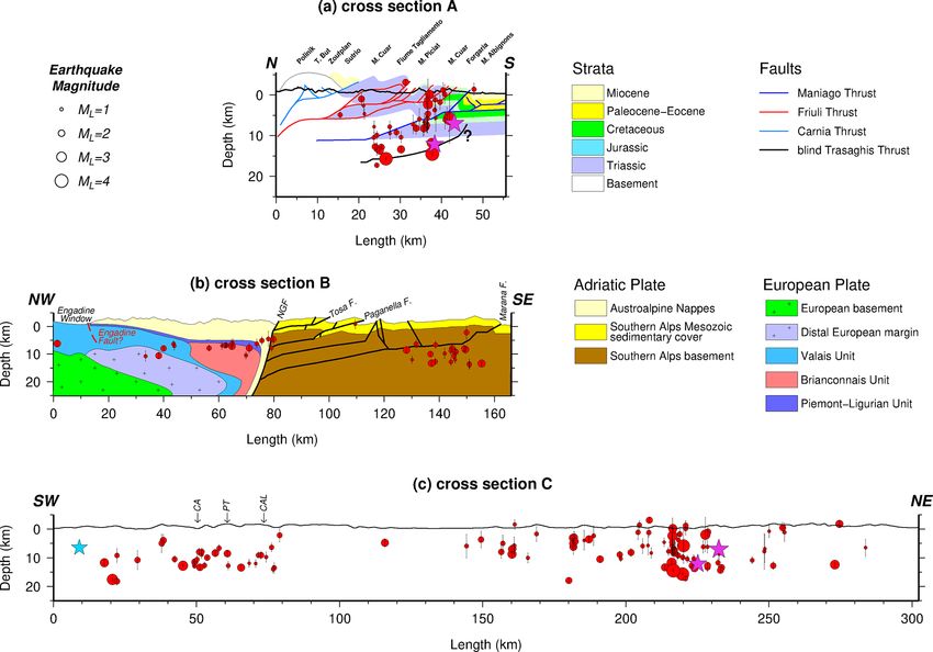
6.3.1 Friuli-Venetia (FV) region in Figs. 11 and 12c; Viganò et al., 2015) was suggested to
have occurred on a low-angle thrust connected to the steep
In accordance with the previous studies (and references Ballino–Garda Fault, which detaches the sedimentary cover
therein Bressan et al., 2016; Reiter et al., 2018) and national (hanging wall) from the underlying crystalline basement in
catalogs, most of the seismicity in our dataset occurs in the its footwall (Viganò et al., 2008, 2013, 2015).
ESA, i.e., within the FV region, coinciding with the eastern The NNW–SSE trending system of vertical strike-slip
part of the deformation front between the Adriatic plate and faults making up the Schio–Vicenza Fault is located between
the PAF. This was also the location of the destructive Friuli the active NW-dipping thrusts of the Giudicarie Belt to the
earthquake of 6 May 1976 (ML 6.4) and its major aftershock west and the NNW-dipping thrusts of the Valsugana thrust
on 15 September 1976 (ML 6.1) (purple stars in Figs. 11 and system to the east. The short observational period of our
12a and c), which are associated with the Susans–Tricesimo network and the low seismicity rate limits the unambigu-
Fault and buried or “blind” Trasaghis thrust, respectively ous association of the earthquakes to specific faults. How-
(Poli et al., 2002; Galadini et al., 2005; Slejko, 2018). We ever, some of the captured seismicity seems to take place
find most earthquakes around 13◦ E (close to the villages of along the Campofontana (CA), Priabona–Trambileno (PT),
Tolmezzo and Gemona) down to a depth of around 17 km and Calisio (CAL) faults (Fig. 12c – western section). The
(Fig. 12a and c – around km 220, corresponding to 13◦ E). Schio–Vicenza fault system is the most active structure in
However, the seismicity is distributed over a wider area (see the GL region and was shown with predominant right-lateral
also Fig. 12c eastern part; between km 140 and 280). As strike-slip mechanism (Viganò et al., 2008).
stated above, a direct connection of individual earthquakes Figure 12b shows the distribution of seismicity superposed
in our dataset to known faults near the surface is difficult. on the main geological structures, which indicates that seis-
Nevertheless, the clustering of seismicity in the FV region micity is focused in its southern part of the GL region. This
between the Alpine frontal thrusts and the Fella–Sava fault in suggests that the most southern and deepest faults (Fig. 12b)
the north suggest that several frontal thrusts and backthrusts remain active, while the more internal fault systems have be-
are active. Moreover, Petersen et al. (2021) shows a dominant come seismically inactive (Verwater et al., 2021). Moreover,
E–W striking thrust mechanism for this region. we observe that the seismicity is deeper than the frontal thrust
According to the fault distribution (and naming) of Gal- modeled from balanced geological cross sections (Fig. 12b;
adini et al. (2005), the seismicity along the cross section A Verwater et al., 2021), similar to observations within the
(Fig. 12a) indicates that the Susans–Tricesimo and Trasaghis FV region (as mentioned above). We interpret this to reflect
faults (and potentially the Maniago thrust) are the most ac- southward propagation of the southern Alpine deformation
tive faults in this region. Most earthquakes are located below front (blind thrusts) towards the Po Plain.
the Maniago thrust, one of the main Alpine frontal thrusts in
the tectonic model of Nussbaum (2000). This suggests that 6.3.3 Lateral variations in clustering of seismicity from
there is an active fault at greater depth (Fig. 12a). We in- the WSA to ESA
terpret this to indicate a blind (i.e., that has not reached the
surface) southward-propagating thrust front. In the profiles A cross section running orogen-parallel from the GL to the
of Galadini et al. (2005) and Merlini et al. (2002) further FV region (Fig. 12c) indicates a similar depth of earthquakes
east, this deeper blind thrust (named Trasaghis thrust in Gal- for both regions. The FV region shows relatively high seis-
adini et al., 2005) reaches the surface, where it offsets Plio– mic activity, located at the junction with the Dinaric Front
Pleistocene sediments. More near-surface activity down to a (Doglioni and Bosellini, 1987). However, in the central part
depth of 6 km can generally be related to the Friuli thrust of cross section C (around km 150 in Fig. 12c), sparse seis-
system (see Nussbaum, 2000, and Fig. 12a). micity may indicate a seismic gap (Anselmi et al., 2011;
Burrato et al., 2008). Alternatively, the sparse seismicity (es-
6.3.2 Giudicarie-Lessini (GL) region pecially at shallow depths) could indicate that deformation
within this area is occurring aseismically, as proposed by
The seismicity in the GL region correlates with the NNE– Barba et al. (2013) and Romano et al. (2019) for the Montello
SSW transpressive fault system of Giudicarie Belt and thrust (Fig. 11). Strain rates within the Montello region are
the NW–SE-trending Schio–Vicenza strike-slip fault system. among the highest within the ESA (Serpelloni et al., 2016),
Seismicity of the Giudicarie fault system is concentrated which combined with its sparse seismicity indicates that the
mainly in the south (southwest of Lake Garda at depths rang- majority of deformation within this area is most likely occur-
ing from a few kilometers down to 15 km; Fig. 11) and is in ring aseismically (Barba et al., 2013).
agreement with Viganò et al. (2015). For this part of the Giu-
dicarie Belt, Viganò et al. (2008) suggested the kinematic
Solid Earth, 12, 1087–1109, 2021 https://doi.org/10.5194/se-12-1087-2021You can also read