Response to the comments of Referee #1 (John Reynolds)
←
→
Page content transcription
If your browser does not render page correctly, please read the page content below
Reconstruction of the 1941 GLOF process chain at Lake Palcacocha (Cordillera Blanca, Perú)

Martin Mergili, Shiva P. Pudasaini, Adam Emmer, Jan-Thomas Fischer, Alejo Cochachin, and Holger Frey

Response to the comments of Referee #1 (John Reynolds)
We would like to thank the reviewer for the constructive remarks. Below, we address each comment in
full detail. Our response is written in blue colour. Changes in the manuscript are highlighted in yellow
colour.

This is an interesting and useful paper that serves two important functions. Firstly, it provides a back
analysis of the 1941 GLOF process chain from Laguna Palcacocha, Peru, that helps an understanding of
the physical processes associated with the event. Secondly, it is a useful demonstration or r.avaflow
software that is fast becoming more widely applied for such studies. The only comment I would make in
this discussion is to expand a little on the detail behind the Laguna 513 situation between 1988 and 1994
as many papers that cite this lake do not report the full story and it merits telling again. Details of the
remediation work undertaken have been described by Reynolds, J.M. 1998. Managing the risks of glacial
flooding at hydro plants. Hydro Review Worldwide, 6(2):18-22; and by Reynolds,J.M., Dolecki, A. and
Portocarrero, C. 1998. The construction of a drainage tunnel as part of glacial lake hazard mitigation at
Hualcán, Cordillera Blanca, Peru. In: Maund, J. & Eddleston, M. (eds.) Geohazards in engineering geology.
Geological Society Engineering Group Special Publication No. 15, pp. 41-48.

In essence, in late 1988, surveying undertaken by local engineers identified that the small moraine dam
impounding Lake 513 was ice cored and that this ice core was subsiding through ablation by∼11
cm/month. It was a simple calculation, therefore, to estimate that by early 1989, the subsidence would
have reduced the freeboard to zero and worse, would have resulted in the moraine dam failing and
being eroded leading to an outburst flood. The local engineers, led by Cesar Portocarrero, identified that
siphoning would be sufficient and practical to reduce the lake level by 3 m or so to alleviate a possible
outburst. However, they had insufficient funds to purchase the necessary siphons. Two days before
Christmas 1988, Cesar phoned me in the UK from Peru to ask if I could help. A few phone calls and
several hours later I had managed to persuade the British Embassy in Lima to provide the necessary
funds. Consequently, within a couple of weeks the siphons had been installed and the lake level lowered.
In 1991, a small ice avalanche, thought to have originated from the hanging glacier perched above the
lake, fell into the lake producing a small displacement wave. However, this was sufficient to breach the
remains of the moraine dam and produce a small outburst flood. It had the consequences of lowering
the water level down to and exposed a solid rock bat that had been beneath the terminal moraine dam.
The new water level was by this time only just below the rim of the rock bar. Ing. Portocarrero began to
design a more permanent mitigation scheme of tunneling through the rock bar to lower the lake by 20
m. In 1993, having been informed of his design, it became apparent that the water hydrostatic pressure
under 20 m plus head of water could rupture the discharge portal end of the proposed tunnel leading to
a greater failure of the distal flank of the rock bar. With emergency funding provided by the British
Government, in late 1993 Reynolds and Dolecki visited the site operations with Ing. Portocarrero. We
came up with a scheme for which the equipment was already on site that required the excavation of a
tiered suite of tunnels whose inflow portals were set 5 m vertically apart, with the uppermost tunnel
being opened first, to lower the lake level down by 5 m; then the second tunnel, for a further 5 m
lowering. Explosives failed to detonate for the break through for the third tunnel, so it was decided to go
for a 10m breach through to the lowermost tunnel, which was established safely and the lake was
successfully lowered by 20 m, thereby creating a freeboard against avalanche push waves and
displacement waves in the case of further avalanche activity. The thinking at that time was that an ice
avalanche would most probably originate from the ice cliff associated with the perched hanging glacier
immediately above the upstream end of the lake. The rock/ice avalanche that occurred in 2010 was from
the uppermost flanks of the back wall above the lake. This was then when it was realised that this
avalanche might have been triggered by thawing of permafrost where the rock face was exposed.
Thankfully, having lowered the lake level by May 994 by 20 m, when the avalanche occurred in 2010, the
exposed rock bar with 20 m of freeboard accommodated most of the 28-m high avalanche push wave,
with only a residual amount overtopping the rock bar. Had the further remediation not have been
undertaken, the consequences of this 2010 would most likely have been far more tragic, with possibly as
many as 5-6,000 fatalities, as defined by the local mayor. Whilst the 2010 GLOF/alluvion caused damage,
especially to the outskirts of the town, there were no casualties.

We are very glad to see that the reviewer likes our paper. We have included the 2010 event at Laguna
513 in the introduction and the discussion of the revised manuscript, referring to the suggested
literature. We have kept the text blocks concerning Laguna 513 brief and concise, clearly relating them
to those aspects also relevant for the present work. A more detailed account of the remediation
measures and the 2010 event would be out of scope here, but could be of great interest for a future
study. In the revised manuscript, we have mainly added the following pieces of text:

Introduction (L64-66):

Most notably, lowering the lake level of Laguna 513 through a system of tunnels in the 1990s has
probably prevented a disaster downstream when a rock-ice avalanche impacted that lake in 2010
(Reynolds, 1998; Reynolds et al., 1998; Schneider et al., 2014).

Discussion (L486-490):

In principle, such an understanding can be transferred to present hazardous situations in order to inform
the design of technical remediation measures. Earlier, measures were not only implemented at Lake
Palcacocha (Portocarrero, 2014), but also at various other lakes such as Laguna 513: a tunnelling scheme
implemented in the 1990s strongly reduced the impacts of the 2010 GLOF process chain (Reynolds, 1998;
Reynolds et al., 1998; Schneider et al., 2014).
1   Reconstruction of the 1941 GLOF process chain at Lake Palcacocha (Cor‐
 2   dillera Blanca, Perú)

 3   Martin Mergili1,2, Shiva P. Pudasaini3, Adam Emmer4, Jan‐Thomas Fischer5, Alejo Co‐
 4   chachin6, and Holger Frey7

 5   1Institute of Applied Geology, University of Natural Resources and Life Sciences (BOKU), Peter-Jordan-Straße 82,
 6   1190 Vienna, Austria
 7   2Geomorphological Systems and Risk Research, Department of Geography and Regional Research, University of Vi-
 8   enna, Universitätsstraße 7, 1010 Vienna, Austria
 9   3   Geophysics Section, Institute of Geosciences, University of Bonn, Meckenheimer Allee 176, 53115 Bonn, Germany
10   4Department of the Human Dimensions of Global Change, Global Change Research Institute, The Czech Academy of
11   Sciences, Bělidla 986/4a, 603 00, Brno, Czech Republic
12   5   Department of Natural Hazards, Austrian Research Centre for Forests (BFW), Rennweg 1, 6020 Innsbruck, Austria
13   6Unidad de Glaciología y Recursos Hídricos, Autoridad Nacional del Agua, Confraternidad Internacional 167, Huaráz,
14   Perú
15   7   Department of Geography, University of Zurich, Winterthurerstrasse 190, 8057 Zurich, Switzerland
16   Correspondence to: M. Mergili (martin.mergili@boku.ac.at)

17   Abstract
18   The Cordillera Blanca in Perú has been the scene of rapid deglaciation for many decades. One of numerous lakes
19   formed in the front of the retreating glaciers is the moraine-dammed Lake Palcacocha, which drained suddenly due to
20   an unknown cause in 1941. The resulting Glacial Lake Outburst Flood (GLOF) led to dam failure and complete drain-
21   age of Lake Jircacocha downstream, and to major destruction and thousands of fatalities in the city of Huaráz at a dis-
22   tance of 23 km. We chose an integrated approach to revisit the 1941 event in terms of topographic reconstruction and
23   numerical back-calculation with the GIS-based open source mass flow/process chain simulation framework r.avaflow.
24   Thereby we consider four scenarios: (A) and (AX) breach of the moraine dam of Lake Palcacocha due to retrogressive
25   erosion, assuming two different fluid characteristics; (B) failure of the moraine dam caused by the impact of a landslide
26   onto the lake; and (C) geomechanical failure and collapse of the moraine dam. The simulations largely yield empirical-
27   ly adequate results with physically plausible parameters, taking the documentation of the 1941 event and previous
28   calculations of future scenarios as reference. Most simulation scenarios indicate travel times between 36 and 70
29   minutes to reach Huaráz, accompanied with peak discharges above 10,000 m³/s. The results of the scenarios indicate
30   that the most likely initiation mechanism would be retrogressive erosion, possibly triggered by a minor impact wave
31   and/or facilitated by a weak stability condition of the moraine dam. However, the involvement of Lake Jircacocha
32   disguises part of the signal of process initiation farther downstream. Predictive simulations of possible future events
33   have to be based on a larger set of back-calculated GLOF process chains, taking into account the expected parameter
34   uncertainties and appropriate strategies to deal with critical threshold effects.

35   Keywords: GLOF, high-mountain lakes, Lake Palcacocha, numerical simulation, process chain, r.avaflow, two-phase
36   flows

                                                               Page 1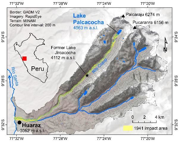
37   1 Introduction
38   Glacial retreat in high-mountain areas often leads, after some lag time (Harrison et al., 2018), to the formation of pro-
39   glacial lakes, which are impounded by moraine dams or bedrock swells. Such lakes may drain suddenly, releasing a
40   large amount of water which may result in complex and potentially catastrophic process chains downstream. Glacial
41   lakes and outburst floods (GLOFs) have been subject of numerous studies covering many mountain regions all around
42   the globe (Hewitt, 1982; Haeberli, 1983; Richardson and Reynolds, 2000; Huggel et al., 2003; Breien et al., 2008;
43   Hewitt and Liu, 2010; Bolch et al., 2011; Mergili and Schneider, 2011; Mergili et al., 2013; Clague and O’Connor, 2014;
44   Emmer et al., 2015, 2016; Sattar et al., 2019a, b; Turzewski et al., 2019).

45   The Cordillera Blanca (Perú) represents the most glacierized mountain chain of the Tropics. Glacial lakes and GLOFs
46   are particularly common there (Carey, 2005). 882 high-mountain lakes were identified by Emmer et al. (2016). Some
47   of these lakes are susceptible to GLOFs (Vilímek et al., 2005; Emmer and Vilímek, 2013, 2014; ANA, 2014; Iturrizaga,
48   2014). A total of 28 geomorphologically effective GLOFs originating from moraine-dammed lakes have been docu-
49   mented (Emmer, 2017). Most recently, GLOFs were recorded at Lake Safuna Alta (2002 – the trigger was a rock ava-
50   lanche into the lake; Hubbard et al., 2005), at Lake Palcacocha (2003 – landslide-induced overtopping of the dam;
51   Vilímek et al., 2005), and at Lake 513 (2010 – triggered by an ice avalanche; Carey et al., 2012). Lake Artizón Alto was
52   hit by a landslide from a moraine in 2012, which resulted in cascading effects involving three more lakes and entrain-
53   ment of a considerable amount of debris in the Artizón Valley and, farther downstream, the Santa Cruz Valley
54   (Mergili et al., 2018a). A pronounced peak in frequency of high-magnitude GLOFs, however, was already observed in
55   the 1940s and 1950s, when lakes of notable size had formed behind steep terminal moraine walls (Emmer et al., 2019).
56   The most prominent and well-documented GLOF in this period occurred on 13 December 1941, when Lake Palcaco-
57   cha in the Quilcay Catchment drained suddenly, leading to a process chain that resulted in at least 1600 fatalities and
58   major destruction in the town of Huaráz 23 km downstream (Broggi, 1942; Oppenheim, 1946; Concha, 1952; Wegner,
59   2014).

60   In the Cordillera Blanca, the local population is highly vulnerable to high-mountain process chains, often induced by
61   GLOFs (Carey, 2005; Hofflinger et al., 2019). In order to mitigate this threat, tens of lakes in the Cordillera Blanca
62   have been remediated through technical measures such as open cuts, artificial dams or tunnels during the last decades
63   (Oppenheim, 1946; Zapata 1978; Portocarrero, 1984; Carey, 2005; Portocarrero, 2014; Emmer et al., 2018). Most nota-
64   bly, lowering the lake level of Laguna 513 through a system of tunnels in the 1990s has probably prevented a disaster
65   downstream when a rock-ice avalanche impacted that lake in 2010 (Reynolds, 1998; Reynolds et al., 1998; Schnei-
66   der et al., 2014). However, the management of GLOF risk is a difficult task (Carey et al., 2014). Anticipation of the
67   impact area and magnitude of GLOF cascades – and, as a consequence, also hazard mapping and the design of technical
68   remediation measures – relies to a large extent on the application of computational mass flow models (GAPHAZ,
69   2017). Important progress was made since the mid-20th Century: various models were developed, and have more re-
70   cently been implemented in simulation software tools (Voellmy, 1955; Savage and Hutter, 1989; Iverson, 1997;
71   Takahashi et al., 2002; Pitman and Le, 2005; McDougall and Hungr, 2004; Pudasaini and Hutter, 2007; Chisolm and
72   McKinney, 2018). Most of these approaches represent single-phase mixture models. Tools like RAMMS (Chris-
73   ten et al., 2010) or FLO-2D were used for the simulation of GLOFs (Mergili et al., 2011). Schneider et al. (2014),
74   Worni et al. (2014), and Somos-Valenzuela et al. (2016) have sequentially coupled two or more tools for simulating
75   landslide – GLOF cascades. However, single-phase models do not describe the interactions between the solid and the
76   fluid phase, or dynamic landslide-lake interactions, in an appropriate way, so that workarounds are necessary
77   (Gabl et al., 2015). Worni et al. (2014) called for integrated approaches. They would have to build on two- or even
78   three-phase models considering water, debris, and ice separately, but also the interactions between the phases and the

                                                               Page 2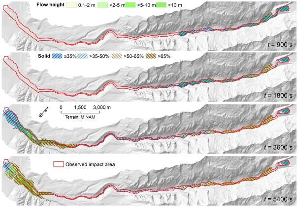
79   flow transformations. Pudasaini (2012) introduced a general two-phase flow model considering mixtures of solid parti-
 80   cles and viscous fluid which has been used for the simulation of computer-generated examples of sub-aqueous land-
 81   slides and particle transport (Kafle et al., 2016, 2019) as well as GLOFs (Kattel et al., 2016).

 82   The recently introduced open source GIS simulation framework r.avaflow (Mergili et al., 2017) applies an extended
 83   version of the approach of Pudasaini (2012). It was used to back-calculate the 2012 Santa Cruz process chain involving
 84   four lakes (Mergili et al., 2018a), and the 1962 and 1970 Huascarán landslides (Mergili et al., 2018b), both in the Cor-
 85   dillera Blanca. These studies identified the capability of that tool to appropriately simulate the transformations at the
 86   boundary of individual processes, where one process transforms to the next, as one of the major challenges. Open is-
 87   sues include the proper understanding of wave generation as a response to landslides impacting high-mountain lakes
 88   and, as a consequence, the quantification of essential parameters such as the volume of overtopping water and the
 89   discharge (Westoby et al., 2014). Further, uncertainties in the model parameters and the initial conditions accumulate
 90   at process boundaries (Schaub et al. 2016), and threshold effects are expected to result in strongly non-linear responses
 91   of the model error (Mergili et al., 2018a, b). In high-energy mass flows, the physical characteristics of the processes
 92   involved are not always understood at the required level of detail (Mergili et al., 2018b).

 93   On the one hand, flow models and simulation tools can help us to better understand some of the key mechanisms of
 94   high-mountain process chains. On the other hand, well documented case studies are important to gain a better under-
 95   standing on which questions can be tackled with simulation tools, and which questions cannot be answered without
 96   further research. In the present work, we explore this field of uncertainty by applying the r.avaflow computational
 97   tool to the 1941 Lake Palcacocha GLOF process chain. Thereby, based on the simulation of different scenarios, we
 98   investigate on the following research questions:

 99         1. What is the most likely release mechanism of initiating the process chain of the 1941 GLOF of Lake Palcaco-
100            cha?

101         2. Are we able to back-calculate this process chain in an empirically adequate way with physically plausible
102            model parameters? Mergili et al. (2018b) reported a trade-off between these two criteria for the simulation of
103            the 1970 Huascarán landslide.

104         3. What are the major challenges in achieving successful (empirically adequate and physically plausible) simula-
105            tions?

106         4. What can we learn with regard to forward calculations of possible future events?

107   In Sect. 2 we depict the local conditions and the documentation of the event. After having introduced the computa-
108   tional framework r.avaflow (Sect. 3), we describe in detail the simulation input (Sect. 4) and our findings (Sect. 5). We
109   discuss the results (Sect. 6) and finally summarize the key points of the research (Sect. 7).

110   2 Lake Palcacocha

111   2.1     Quilcay catchment and Cojup Valley

112   Lake Palcacocha is part of a proglacial system in the headwaters of the Cojup Valley in the Cordillera Blanca, Perú
113   (Fig. 1). This system was – and is still – shaped by the glaciers originating from the southwestern slopes of Nevado
114   Palcaraju (6,264 m a.s.l.) and Nevado Pucaranra (6,156 m a.s.l.). A prominent horseshoe-shaped ridge of lateral and
115   terminal moraines marks the extent of the glacier during the first peak of the Little Ice Age, dated using lichenometry
116   to the 17th Century (Emmer, 2017). With glacier retreat, the depression behind the moraine ridge was filled with a

                                                                 Page 3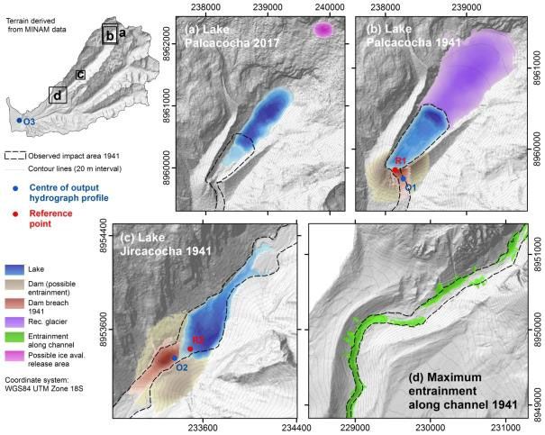
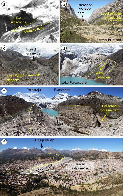
117   lake, named Lake Palcacocha. A photograph taken by Hans Kinzl in 1939 (Kinzl and Schneider, 1950) indicates a lake
118   level of 4,610 m a.s.l., allowing surficial outflow (Fig. 2a). Using this photograph, Vilímek et al. (2005) estimated a lake
119   volume between 9 and 11 million m³ at that time, whereas an unpublished estimate of the Autoridad Nacional del
120   Agua (ANA) arrived at approx. 13.1 million m³. It is assumed that the situation was essentially the same at the time of
121   the 1941 GLOF (Sect. 2.2).

122   The Cojup Valley is part of the Quilcay catchment, draining towards southwest to the city of Huaráz, capital of the
123   department of Ancash located at 3,090 m a.s.l. at the outlet to the Río Santa Valley (Callejon de Huaylas). The distance
124   between Lake Palcacocha and Huaráz is approx. 23 km, whereas the vertical drop is approx. 1,500 m. The Cojup Val-
125   ley forms a glacially shaped high-mountain valley in its upper part whilst cutting through the promontory of the Cor-
126   dillera Blanca in its lower part. 8 km downstream from Lake Palcacocha (15 km upstream of Huaráz), the landslide-
127   dammed Lake Jircacocha (4.8 million m³; Vilímek et al., 2005) existed until 1941 (Andres et al., 2018). The remnants
128   of this lake are still clearly visible in the landscape in 2017, mainly through the change in vegetation and the presence
129   of fine lake sediments (Fig. 2b). Table 1 summarizes the major characteristics of Lake Palcacocha and Lake Jircacocha
130   before the 1941 GLOF.

131   2.2   1941 multi‐lake outburst flood from Lake Palcacocha

132   On 13 December 1941 part of the city of Huaráz was destroyed by a catastrophic GLOF-induced debris and mud flow,
133   with thousands of fatalities. Portocarrero (1984) gives a number of 4000 deaths, Wegner (2014) a number of 1800; but
134   this type of information has to be interpreted with care (Evans et al., 2009). The disaster was the result of a multi-lake
135   outburst flood in the upper part of the Cojup Valley. Sudden breach of the dam and the drainage of Lake Palcacocha
136   (Figs. 2c and e) led to a mass flow proceeding down the valley. Part of the eroded dam material, mostly coarse materi-
137   al, blocks and boulders, was deposited directly downstream from the moraine dam, forming an outwash fan typical for
138   moraine dam failures (Fig. 2c), whereas additional solid material forming the catastrophic mass flow was most likely
139   eroded further along the flow path (both lateral and basal erosion were observed; Wegner, 2014). The impact of the
140   flow on Lake Jircacocha led to overtopping and erosion of the landslide dam down to its base, leading to the complete
141   and permanent disappearance of this lake. The associated uptake of the additional water and debris increased the en-
142   ergy of the flow, and massive erosion occurred in the steeper downstream part of the valley, near the city of Huaráz.
143   Reports by the local communities indicate that the valley was deepened substantially, so that the traffic between vil-
144   lages was interrupted. According to Somos-Valenzuela et al. (2016), the valley bottom was lowered by as much as
145   50 m in some parts.

146   The impact area of the 1941 multi-GLOF and the condition of Lake Palcacocha after the event are well documented
147   through aerial imagery acquired in 1948 (Fig. 3). The image of Hans Kinzl acquired in 1939 (Fig. 2a) is the only record
148   of the status before the event. Additional information is available through eyewitness reports (Wegner, 2014). Howev-
149   er, as Lake Palcacocha is located in a remote, uninhabited area, no direct estimates of travel times or associated flow
150   velocities are available. Also the trigger of the sudden drainage of Lake Palcacocha remains unclear. Two mechanisms
151   appear most likely: (i) retrogressive erosion, possibly triggered by an impact wave related to calving or an ice ava-
152   lanche, resulting in overtopping of the dam (however, Vilímek et al., 2005 state that there are no indicators for such
153   an impact); or (ii) internal erosion of the dam through piping, leading to the failure.

154   2.3   Lake evolution since 1941

155   As shown on the aerial images from 1948, Lake Palcacocha was drastically reduced to a small remnant proglacial pond,
156   impounded by a basal moraine ridge within the former lake area, at a water level of 4563 m a.s.l., 47 m lower than

                                                                Page 4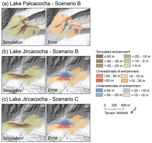
157   before the 1941 event (Fig. 3a). However, glacial retreat during the following decades led to an increase of the lake
158   area and volume (Vilímek et al., 2005). After reinforcement of the dam and the construction of an artificial drainage in
159   the early 1970s, a lake volume of 514,800 m³ was derived from bathymetric measurements (Ojeda, 1974). In 1974, two
160   artificial dams and a permanent drainage channel were installed, stabilizing the lake level with a freeboard of 7 m to
161   the dam crest (Portocarrero, 2014). By 2003, the volume had increased to 3.69 million m³ (Zapata et al., 2003). In the
162   same year, a landslide from the left lateral moraine caused a minor flood wave in the Cojup Valley (Fig. 2d). In 2016,
163   the lake volume had increased to 17.40 million m³ due to continued deglaciation (ANA, 2016). The potential of fur-
164   ther growth is limited since, as of 2017, Lake Palcacocha is only connected to a small regenerating glacier. Further, the
165   lake level is lowered artificially, using a set of siphons (it decreased by 3 m between December 2016 and July 2017).
166   Table 1 summarizes the major characteristics of Lake Palcacocha in 2016. The overall situation in July 2017 is illustrat-
167   ed in Fig. 2c.

168   2.4   Previous simulations of possible future GLOF process chains

169   Due to its history, recent growth, and catchment characteristics, Lake Palcacocha is considered hazardous for the
170   downstream communities, including the city of Huaráz (Fig. 2e). Whilst Vilímek et al (2005) point out that the lake
171   volume would not allow an event comparable to 1941, by 2016 the lake volume had become much larger than the
172   volume before 1941 (ANA, 2016). Even though the lower potential of dam erosion (Somos-Valenzuela et al., 2016) and
173   the non-existence of Lake Jircacocha make a 1941-magnitude event appear unlikely, the steep glacierized mountain
174   walls in the back of the lake may produce ice or rock-ice avalanches leading to impact waves, dam overtopping, ero-
175   sion, and subsequent mass flows. Investigations by Klimeš et al. (2016) of the steep lateral moraines surrounding the
176   lake indicate that failures and slides from moraines are possible at several sites, but do not have the potential to create
177   a major overtopping wave, partly due to the elongated shape of the lake. Rivas et al. (2015) elaborated on the possible
178   effects of moraine-failure induced impact waves. Recently, Somos-Valenzuela et al. (2016) have used a combination of
179   simulation approaches to assess the possible impact of process chains triggered by ice avalanching into Lake Palcaco-
180   cha on Huaráz. They considered three scenarios of ice avalanches detaching from the slope of Palcaraju (0.5, 1.0, and
181   3.0 million m³) in order to create flood intensity maps and to indicate travel times of the mass flow to various points of
182   interest. For the large scenario, the mass flow would reach the uppermost part of the city of Huaráz after approx.
183   1 h 20 min, for the other scenarios this time would increase to 2 h 50 min (medium scenario) and 8 h 40 min (small
184   scenario). Particularly for the large scenario, a high level of hazard is identified for a considerable zone near the Quil-
185   cay River, whereas zones of medium or low hazard become more abundant with the medium and small scenarios, or
186   with the assumption of a lowered lake level (Somos-Valenzuela et al., 2016). In addition, Chisolm and McKinney
187   (2018) analyzed the dynamics impulse waves generated by avalanches using FLOW-3D. A similar modelling approach
188   was applied by Frey et al. (2018) to derive a map of GLOF hazard for the Quilcay catchment. For Lake Palcacocha the
189   same ice avalanche scenarios as applied by Somos-Valenzuela et al. (2016) were employed, with correspondingly com-
190   parable results in the Cojup Valley and for the city of Huaráz.

191   3 The r.avaflow computational tool
192   r.avaflow is an open source tool for simulating the dynamics of complex mass flows in mountain areas. It employs a
193   two-phase model including solid particles and viscous fluid, making a difference to most other mass flow simulation
194   tools which build on one-phase mixture models. r.avaflow considers the interactions between the phases as well as
195   erosion and entrainment of material from the basal surface. Consequently, it is well-suited for the simulation of com-

                                                               Page 5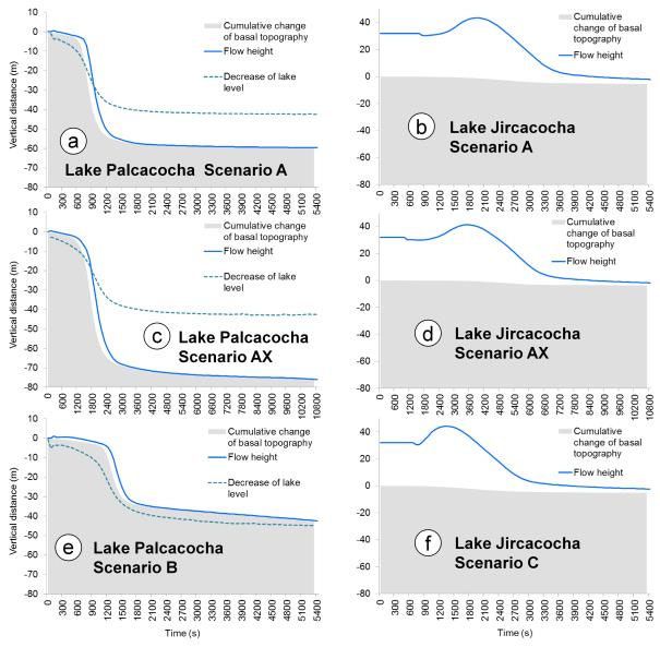
196 plex, cascading flow-type landslide processes. The r.avaflow framework is introduced in detail by Mergili et al. (2017),
197 only those aspects relevant for the present work are explained here.
198 The Pudasaini (2012) two-phase flow model is used for propagating mass flows from at least one defined release area
199 through a Digital Terrain Model (DTM). Flow dynamics is computed through depth-averaged equations describing the
200 conservation of mass and momentum for both solid and fluid. The solid stress is computed on the basis of the Mohr-
201 Coulomb plasticity, whereas the fluid is treated with a solid-volume-fraction-gradient-enhanced non-Newtonian vis-
202 cous stress. Virtual mass due to the relative motion and acceleration, and generalized viscous drag, account for the
203 strong transfer of momentum between the phases. Also buoyancy is considered. The momentum transfer results in
204 simultaneous deformation, separation, and mixing of the phases (Mergili et al., 2018a). Pudasaini (2012) gives a full
205 description of the set of equations.
206 Certain enhancements are included, compared to the original model: for example, drag and virtual mass are computed
207 according to extended analytical functions constructed by Pudasaini (2019a, b). Additional (complementary) function-
208 alities include surface control, diffusion control, and basal entrainment (Mergili et al., 2017, 2018a, 2019). A conceptu-
209 al model is used for entrainment: thereby, the empirically derived entrainment coefficient CE is multiplied with the
210 flow kinetic energy:
211 q E,s C E Ts Tf s,E , q E,f C E Ts Tf 1 s,E . (1)
212 qE,s and qE,f (m s-1) are the solid and fluid entrainment rates, Ts and Tf (J) are the solid and fluid kinetic energies, and αs,E
213 is the solid fraction of the entrainable material (Mergili et al., 2019). Flow heights and momenta as well as the change
214 of elevation of the basal surface are updated at each time step (Mergili et al., 2017).
215 Any desired combination of solid and fluid release and entrainable heights can be defined. The main results are raster
216 maps of the evolution of solid and fluid flow heights, velocities, and entrained heights in time. Pressures and kinetic
217 energies are derived from the flow heights and velocities. Output hydrographs can be generated as an additional op-
218 tion (Mergili et al., 2018a). Spatial discretization works on the basis of GIS raster cells: the flow propagates between
219 neighbouring cells during each time step. The Total Variation Diminishing Non-Oscillatory Central Differencing
220 (TVD-NOC) Scheme (Nessyahu and Tadmor, 1990; Tai et al., 2002; Wang et al., 2004) is employed for solving the
221 model equations. This approach builds on a staggered grid, in which the system is shifted half the cell size during each
222 step in time (Mergili et al., 2018b).
223 r.avaflow operates as a raster module of the open source software GRASS GIS 7 (GRASS Development Team, 2019),
224 employing the programming languages Python and C as well as the R software (R Core Team, 2019). More details
225 about r.avaflow are provided by Mergili et al. (2017).
226 4 Simulation input
227 The simulations build on the topography, represented by a DTM, and on particular sets of initial conditions and model
228 parameters. For the DTM, we use a 5 m resolution Digital Elevation Model provided by the Peruvian Ministry of Envi-
229 ronment, MINAM (Horizons, 2013). It was deduced from recent stereo aerial photographs and airborne LiDAR. The
230 DEM is processed in order to derive a DTM representing the situation before the 1941 event. Thereby, we neglect the
231 possible error introduced by the effects of vegetation or buildings, and focus on the effects of the lakes and of erosion
232 (Fig. 4):
233 1. For the area of Lake Palcacocha the elevation of the lake surface is replaced by a DTM of the lake bathymetry
234 derived from ANA (2016). Possible sedimentation since that time is neglected. The photograph of Hans Kinzl
Page 6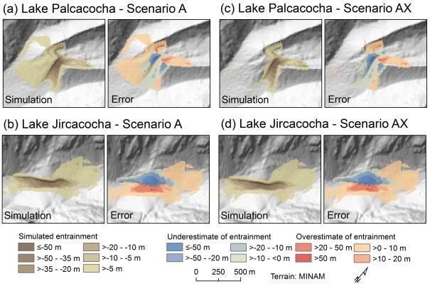
235           from 1939 (Fig. 2a) is used to reconstruct the moraine dam before the breach, and the glacier at the same time.
236           As an exact positioning of the glacier terminus is not possible purely based on the photo, the position is opti-
237           mized towards a lake volume of approx. 13 million m³, following the estimate of ANA. It is further assumed
238           that there was surficial drainage of Lake Palcacocha as suggested by Fig. 2a, i.e. the lowest part of the moraine
239           crest is set equal to the former lake level of 4,610 m a.s.l (Fig. 4b).
240       2. Also for Lake Jircacocha, surficial overflow is assumed (a situation that is observed for most of the recent land-
241           slide-dammed lakes in the Cordillera Blanca). On this basis the landslide dam before its breach is reconstruct-
242           ed, guided by topographic and geometric considerations. The lowest point of the dam crest is set to
243           4,130 m a.s.l. (Fig. 4c).
244       3. Erosional features along the flow channel are assumed to largely relate to the 1941 event. These features are
245           filled accordingly (see Table 2 for the filled volumes). In particular, the flow channel in the lower part of the
246           valley, reportedly deepened by up to 50 m in the 1941 event (Vilímek et al., 2005), was filled in order to repre-
247           sent the situation before the event in a plausible way (Fig. 4d).

248   All lakes are considered as fluid release volumes in r.avaflow. The initial level of Lake Palcacocha in 1941 is set to
249   4,610 m a.s.l., whereas the level of Lake Jircacocha is set to 4,129 m a.s.l. The frontal part of the moraine dam im-
250   pounding Lake Palcacocha and the landslide dam impounding Lake Jircacocha are considered as entrainable volumes.
251   Further, those areas filled up along the flow path (Fig. 4d) are considered entrainable, mainly following Vilímek et al.
252   (2005). However, as it is assumed that part of the material was removed through secondary processes or afterwards,
253   only 75% of the added material are allowed to be entrained. All entrained material is considered 80% solid and 20%
254   fluid per volume.

255   The reconstructed lake, breach, and entrainable volumes are shown in Tables 1 and 2. The glacier terminus in 1941
256   was located in an area where the lake depth increases by several tens of metres, so that small misestimates in the posi-
257   tion of the glacier tongue may result in large misestimates of the volume, so that some uncertainty has to be accepted.

258   As the trigger of the sudden drainage of Lake Palcacocha is not clear, we consider four scenarios, based on the situa-
259   tion before the event as shown in the photo taken by Hans Kinzl, experiences from other documented GLOF events in
260   the Cordillera Blanca (Schneider et al., 2014; Mergili et al., 2018a), considerations by Vilímek et al. (2005), Portocarre-
261   ro (2014), and Somos-Valenzuela et al. (2016), as well as geotechnical considerations:

262      A     Retrogressive erosion, possibly induced by minor or moderate overtopping. This scenario is related to a pos-
263            sible minor impact wave, caused for example by calving of ice from the glacier front, an increased lake level
264            due to meteorological reasons, or a combination of these factors. In the simulation, the process chain is start-
265            ed by cutting an initial breach into the dam in order to initiate overtopping and erosion. The fluid phase is
266            considered as pure water.

267      AX    Similar to Scenario A, but with the second phase considered a mixture of fine mud and water. For this pur-
268            pose, density is increased to 1,100 instead of 1,000 kg m-3, and a yield strength of 5 Pa is introduced (Dom-
269            nik et al., 2013; Pudasaini and Mergili, 2019; Table 3). For simplicity, we still refer to this mixture as a fluid.
270            Such changed phase characteristics may be related to the input of fine sediment into the lake water (e.g.
271            caused by a landslide from the lateral moraine as triggering event), but are mainly considered here in order
272            to highlight the effects of uncertainties in the definition and parameterization of the two-phase mixture flow.

273      B     Retrogressive erosion, induced by violent overtopping. This scenario is related to a large impact wave caused
274            by a major rock/ice avalanche or ice avalanche rushing into the lake. In the simulation, the process chain is
275            initiated through a hypothetic landslide of 3 million m³ of 75% solid and 25% fluid material, following the

                                                                  Page 7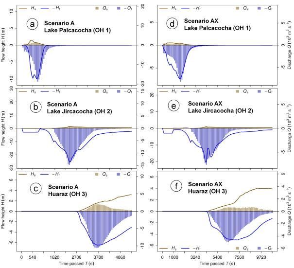
276            large scenario of Somos-Valenzuela et al. (2016) in terms of volume and release area. In order to be consistent
277            with Scenario A, fluid is considered as pure water.

278      C     Internal erosion-induced failure of the moraine dam. Here, the process chain is induced by the collapse of
279            the entire reconstructed breach volume (Fig. 4b). In the simulation, this is done by considering this part of
280            the moraine not as entrainable volume, but as release volume (80% solid, 20% fluid, whereby fluid is again
281            considered as pure water).

282   Failure of the dam of Lake Jircacocha is assumed having occurred through overtopping and retrogressive erosion, in-
283   duced by the increased lake level and a minor impact wave from the flood upstream. No further assumptions of the
284   initial conditions are required in this case.

285   The model parameter values are selected in accordance with experiences gained from previous simulations with
286   r.avaflow for other study areas, and are summarized in Table 3. Three parameters mainly characterizing the flow fric-
287   tion (basal friction of solid δ, ambient drag coefficient CAD, and fluid friction coefficient CFF) and the entrainment coef-
288   ficient CE are optimized in a spatially differentiated way to maximize the empirical adequacy of the simulations in
289   terms of estimates of impact areas, erosion depths, and flow and breach volumes. As no travel times or velocities are
290   documented for the 1941 event, we use the values given by Somos-Valenzuela et al. (2016) as a rough reference. Vary-
291   ing those four parameters while keeping the others constant helps us to capture variability while minimizing the de-
292   grees of freedom, remaining aware of possible equifinality issues (Beven, 1996; Beven and Freer, 2001).

293   A particularly uncertain parameter is the empirical entrainment coefficient CE (Eq. 1). In order to optimize CE, we
294   consider (i) successful prediction of the reconstructed breach volumes; and (ii) correspondence of peak discharge with
295   published empirical equations on the relation between peak discharge, and lake volume and dam height (Walder and
296   O’Connor, 1997). Table 4 summarizes these equations for moraine dams (applied to Lake Palcacocha) and landslide
297   dams (applied to Lake Jircacocha), and the values obtained for the regression and the envelope, using the volumes of
298   both lakes. We note that Table 4 reveals very large differences – roughly one order of magnitude – between regression
299   and envelope. In case of the breach of the moraine dam of Lake Palcacocha, we consider an extreme event due to the
300   steep, poorly consolidated, and maybe soaked moraine, with a peak discharge close to the envelope (approx..
301   15,000 m3 s-1). For Lake Jircacocha, in contrast, the envelope values of peak discharge do not appear realistic. However,
302   due to the high rate of water inflow from above, a value well above the regression line still appears plausible, even
303   though the usefulness of the empirical laws for this type of lake drainage can be questioned. The value of CE optimized
304   for the dam of Lake Jircacocha is also used for entrainment along the flow path.

305   All of the computational experiments are run with 10 m spatial resolution. Only flow heights ≥25 cm are considered
306   for visualization and evaluation. We now describe one representative simulation result for each of the considered sce-
307   narios, thereby spanning the most plausible and empirically adequate field of simulations.

308   5 r.avaflow simulation results

309   5.1    Scenario A – Event induced by overtopping; fluid without yield strength

310   Outflow from Lake Palcacocha starts immediately, leading to (1) lowering of the lake level and (2) retrogressive ero-
311   sion of the moraine dam. The bell-shaped fluid discharge curve at the hydrograph profile O1 (Fig. 4) reaches its peak
312   of 18,700 m³ s-1 after approx. 780 s, and then decreases to a small residual (Fig. 5a). Channel incision happens quickly –
313   53 m of lowering of the terrain at the reference point R1 occurs in the first less than 1200 s, whereas the lowering at
314   the end of the simulation is 60 m (Fig. 6a). This number represents an underestimation, compared to the reference

                                                                Page 8
315 value of 76 m (Table 2). The lake level decreases by 42 m, whereby 36.5 m of the decrease occur within the first
316 1200 s. The slight underestimation, compared to the reference value of 47 m of lake level decrease, is most likely a
317 consequence of uncertainties in the topographic reconstruction. A total amount of 1.5 million m³ is eroded from the
318 moraine dam of Lake Palcacocha, corresponding to an underestimation of 22%, compared to the reconstructed breach
319 volume. Underestimations mainly occur at both sides of the lateral parts of the eroded channel near the moraine crest
320 – an area where additional post-event erosion can be expected, so that the patterns and degree of underestimation
321 appear plausible (Fig. 7a). In contrast, some overestimation of erosion occurs in the inner part of the dam. For numeri-
322 cal reasons, some minor erosion is also simulated away from the eroded channel. The iterative optimization procedure
323 results in an entrainment coefficient CE = 10-6.75.
324 The deposit of much of the solid material eroded from the moraine dam directly downstream from Lake Palcacocha, as
325 observed in the field (Fig. 2c), is reasonably well reproduced by this simulation, so that the flow proceeding down-
326 valley is dominated by the fluid phase (Fig. 8). It reaches Lake Jircacocha after t = 840 s (Fig. 5b). As the inflow occurs
327 smoothly, there is no impact wave in the strict sense, but it is rather the steadily rising water level (see Fig. 6b for the
328 evolution of the water level at the reference point R2) inducing overtopping and erosion of the dam. This only starts
329 gradually after some lag time, at approx. t = 1,200 s. The discharge curve at the profile O2 (Fig. 4) reaches its pro-
330 nounced peak of 750 m³ s-1 solid and 14,700 m³ s-1 fluid material at t = 2,340 s, and then tails off slowly.
331 In the case of Lake Jircacocha, the simulated breach is clearly shifted south, compared to the observed breach. With
332 the optimized value of the entrainment coefficient CE = 10-7.15, the breach volume is underestimated by 24%, compared
333 to the reconstruction (Fig. 7b). Also here, this intentionally introduced discrepancy accounts for some post-event ero-
334 sion. However, we note that volumes are uncertain as the reconstruction of the dam of Lake Jircacocha – in contrast to
335 Lake Palcacocha – is a rough estimation due to lacking reference data.
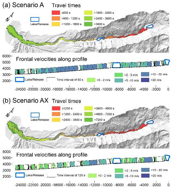
336 Due to erosion of the dam of Lake Jircacocha, and also erosion of the valley bottom and slopes, the solid fraction of the
337 flow increases considerably downstream. Much of the solid material, however, is deposited in the lateral parts of the
338 flow channel, so that the flow arriving at Huaráz is fluid-dominated again (Fig. 8). The front enters the alluvial fan of
339 Huaráz at t = 2,760 s, whereas the broad peak of 10,500 m³ s-1 of fluid and 2,000 m³ s-1 of solid material (solid fraction
340 of 16%) is reached in the period between 3,600 and 3,780 s (Fig. 4; Fig. 5c). Discharge decreases steadily afterwards. A
341 total of 2.5 million m³ of solid and 14.0 million m³ of fluid material pass the hydrograph profile O3 until t = 5,400 s.
342 Referring only to the solid, this is less material than reported by Kaser and Georges (2003). However, (i) there is still
343 some material coming after, and (ii) pore volume has to be added to the solid volume, so that the order of magnitude
344 of material delivered to Huaráz corresponds to the documentation in a better way. Still, the solid ratio of the hydro-
345 graph might represent an underestimation.
346 As prescribed by the parameter optimization, the volumes entrained along the channel are in the same order of mag-
347 nitude, but lower than the reconstructed volumes summarized in Table 2: 0.7 million m3 of material are entrained
348 upstream and 1.5 million m3 downstream of Lake Jircacocha, and 5.3 million m³ in the promontory. Fig. 9a summariz-
349 es the travel times and the flow velocities of the entire process chain. Frontal velocities mostly vary between 5 m s-1
350 and 20 m s-1, with the higher values in the steeper part below Lake Jircacocha. The low and undefined velocities di-
351 rectly downstream of Lake Jircacocha reflect the time lag of substantial overtopping. The key numbers in terms of
352 times, discharges, and volumes are summarized in Table 5.
353 5.2 Scenario AX – Event induced by overtopping; fluid with yield strength
354 Adding a yield strength of τy = 5 Pa to the characteristics of the fluid substantially changes the temporal rather than
355 the spatial evolution of the process cascade. As the fluid now behaves as fine mud instead of water and is more re-
Page 9356 sistant to motion, velocities are lower, travel times are much longer, and the entrained volumes are smaller than in the
357 Scenario A (Fig. 9b; Table 5). The peak discharge at the outlet of Lake Palcacocha is reached at t = 1,800 s. Fluid peak
358 discharge of 8,200 m³ s-1 is less than half the value yielded in Scenario A (Fig. 5d). The volume of material eroded from
359 the dam is only slightly smaller than in Scenario A (1.4 versus 1.5 million m³). The numerically induced false positives
360 with regard to erosion observed in Scenario A are not observed in Scenario AX, as the resistance to oscillations in the
361 lake is higher with the added yield strength (Fig. 7c). Still, the major patterns of erosion and entrainment are the same.
362 Interestingly, erosion is deeper in Scenario AX, reaching 76 m at the end of the simulation (Fig. 6c) and therefore the
363 base of the entrainable material (Table 2). This is most likely a consequence of the spatially more concentrated flow
364 and therefore higher erosion rates along the centre of the breach channel, with less lateral spreading than in Scenar-
365 io A.
366 Consequently, also Lake Jircacocha is reached later than in Scenario A (Fig. 6d), and the peak discharge at its outlet is
367 delayed (t = 4,320 s) and lower (7,600 m³ s-1 of fluid and 320 m³ s-1 of solid material) (Fig. 5e). 2.0 million m³ of materi-
368 al are entrained from the dam of Lake Jircacocha, with similar spatial patterns as in Scenario A (Fig. 7d). Huaráz is
369 reached after t = 4,200 s, and the peak discharge of 5,000 m³ s-1 of fluid and 640 m³ s-1 of solid material at O3 occurs
370 after t = 6,480 s (Fig. 5f). This corresponds to a solid ratio of 11%. Interpretation of the solid ratio requires care here as
371 the fluid is defined as fine mud, so that the water content is much lower than the remaining 89%. The volumes en-
372 trained along the flow channel are similar in magnitude to those obtained in the simulation of Scenario A (Table 5).
373 5.3 Scenario B – Event induced by impact wave
374 Scenario B is based on the assumption of an impact wave from a 3 million m³ landslide. However, due to the relatively
375 gently-sloped glacier tongue heading into Lake Palcacocha at the time of the 1941 event (Figs. 2a and 4b), only a small
376 fraction of the initial landslide volume reaches the lake, and impact velocities and energies are reduced, compared to a
377 direct impact from the steep slope. Approx. 1 million m³ of the landslide have entered the lake until t = 120 s, an
378 amount which only slightly increases thereafter. Most of the landslide deposits on the glacier surface. Caused by the
379 impact wave, discharge at the outlet of Lake Palcacocha (O1) sets on at t = 95 s and, due to overtopping of the impact
380 wave, immediately reaches a relatively moderate first peak of 7,000 m³ s-1 of fluid discharge. The main peak of
381 16,900 m³ s-1 of fluid and 2,000 m³ s-1 of solid discharge occurs at t = 1,200 s due do the erosion of the breach channel.
382 Afterwards, discharge decreases relatively quickly to a low base level (Fig. 10a). The optimized value of CE = 10-6.75 is
383 used also for this scenario. The depth of erosion along the main path of the breach channel is clearly less than in the
384 Scenario A (Fig. 6e). However, Table 5 shows a higher volume of eroded dam material than the other scenarios. These
385 two contradicting patterns are explained by Fig. 11a: the overtopping due to the impact wave does not only initiate
386 erosion of the main breach, but also of a secondary breach farther north. Consequently, discharge is split among the
387 two breaches and therefore less concentrated, explaining the lower erosion at the main channel despite a larger total
388 amount of eroded material. The secondary drainage channel can also be deduced from observations (Fig. 3a), but has
389 probably played a less important role than suggested by this simulation.
390 The downstream results of Scenario B largely correspond to the results of the Scenario A, with some delay partly relat-
391 ed to the time from the initial landslide to the overtopping of the impact wave. Discharge at the outlet of Lake Jircaco-
392 cha peaks at t = 2,700 s (Fig. 10b), and the alluvial fan of Huaráz is reached after 3,060 s (Fig. 10c). The peak discharges
393 at O2 and O3 are similar to those obtained in the Scenario A. The erosion patterns at the dam of Lake Jircacocha
394 (again, CE = 10-7.15) very much resemble those yielded with the scenarios A and AX (Fig. 11b), and so does the volume
395 of entrained dam material (2.2 million m³). The same is true for the 2.5 million m³ of solid and 13.9 million m³ of fluid
396 material entering the area of Huaráz until t = 5,400 s, according to this simulation.
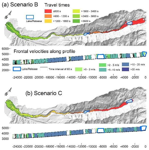
Page 10397 Also in this scenario, the volumes entrained along the flow channel are very similar to those obtained in the simula-
398 tion of Scenario A. The travel times and frontal velocities – resembling the patterns obtained in Scenario A, with the
399 exception of the delay – are shown in Fig. 12a, whereas Table 5 summarizes the key numbers in terms of times, vol-
400 umes, and discharges.
401 5.4 Scenario C – Event induced by dam collapse
402 In Scenario C, we assume that the breached part of the moraine dam collapses, the collapsed mass mixes with the wa-
403 ter from the suddenly draining lake, and flows downstream. The more sudden and powerful release, compared to the
404 two other scenarios, leads to higher frontal velocities and shorter travel times (Fig. 12b; Table 5).
405 In contrast to the other scenarios, impact downstream starts earlier, as more material is released at once, instead of
406 steadily increasing retrogressive erosion and lowering of the lake level. The fluid discharge at O1 peaks at almost
407 40,000 m³ s-1 (Fig. 10d) rapidly after release. Consequently, Lake Jircacocha is reached already after 720 s, and the im-
408 pact wave in the lake evolves more quickly than in all the other scenarios considered (Fig. 6f). The lake drains with a
409 peak discharge of 15,400 m³ s-1 of fluid and 830 m³ s-1 of solid material after 1,680–1,740 s (Fig. 10e). In contrast to the
410 more rapid evolution of the process chain, discharge magnitudes are largely comparable to those obtained with the
411 other scenarios. The same is true for the hydrograph profile O3: the flow reaches the alluvial fan of Huaráz after
412 t = 2,160 s, with a peak discharge slightly exceeding 10,000 m³ s-1 of fluid and 2,000 m³ s-1 of solid material between
413 t = 2,940 s and 3,240 s. 2.7 million m³ of solid and 14.6 million m³ of fluid material enter the area of Huaráz until
414 t = 5,400 s, which is slightly more than in the other scenarios, indicating the more powerful dynamics of the flow (Ta-
415 ble 5). The fraction of solid material arriving at Huaráz remains low, with 16% solid at peak discharge and 15% in to-
416 tal. Again, the volumes entrained along the flow channel are very similar to those obtained with the simulations of the
417 other scenarios (Table 5).
418 6 Discussion
419 6.1 Possible trigger of the GLOF process chain
420 In contrast to other GLOF process chains in the Cordillera Blanca, such as the 2010 event at Laguna 513 (Schneider et
421 al., 2014), which was clearly triggered by an ice-rock avalanche into the lake, there is disagreement upon the trigger of
422 the 1941 multi-lake outburst flood in the Quilcay catchment. Whereas, according to contemporary reports, there is no
423 evidence of a landslide (for example, ice avalanche) impact onto the lake (Vilímek et al., 2005; Wegner, 2014), and
424 dam rupture would have been triggered by internal erosion, some authors postulate an at least small impact starting
425 the process chain (Portocarrero, 2014; Somos-Valenzuela et al., 2016).
426 Each of the three assumed initiation mechanisms of the 1941 event, represented by the Scenarios A/AX, B, and C,
427 yields results which are plausible in principle. We consider a combination of all three mechanisms a likely cause of
428 this extreme process chain. Overtopping of the moraine dam, possibly related to a minor impact wave, leads to the
429 best correspondence of the model results with the observation, documentation, and reconstruction. Particularly the
430 signs of minor erosion of the moraine dam north of the main breach (Fig. 3a) support this conclusion: a major impact
431 wave, resulting in violent overtopping of the entire frontal part of the moraine dam, would supposedly also have led to
432 more pronounced erosion in that area, as to some extent predicted by the Scenario B. There is also no evidence for
433 strong landslide-glacier interactions (massive entrainment of ice or even detachment of the glacier tongue) which
434 would be likely scenarios in the case of a very large landslide. Anyway, the observations do not allow for substantial
435 conclusions on the volume of a hypothetic triggering landslide: as suggested by Scenario B, even a large landslide from
Page 11436 the slopes of Palcaraju or Pucaranra could have been partly alleviated on the rather gently sloped glacier tongue be-
437 tween the likely release area and Lake Palcacocha.
438 The minor erosional feature north of the main breach was already visible in the photo of Kinzl (Fig. 2a), possibly indi-
439 cating an earlier, small GLOF. It remains unclear whether it was reactivated in 1941. Such a reactivation could only be
440 directly explained by an impact wave, but not by retrogressive erosion only (A/AX) or internal failure of the dam (C) –
441 so, more research is needed here. The source area of a possible impacting landslide could have been the slopes of Pal-
442 caraju or Pucaranra (Fig. 1), or the calving glacier front (Fig. 2a). Attempts to quantify the most likely release volume
443 and material composition would be considered speculative due to the remaining difficulties in adequately simulating
444 landslide-(glacier-)lake interactions (Westoby et al., 2014). Further research is necessary in this direction. In any case,
445 a poor stability condition of the dam (factor of safety ~ 1) could have facilitated the major retrogressive erosion of the
446 main breach. A better understanding of the hydro-mechanical load applied by a possible overtopping wave and the
447 mechanical strength of the moraine dam could help to resolve this issue.
448 The downstream patterns of the flow are largely similar for each of the scenarios A, AX, B, and C, with the exception
449 of travel times and velocities. Interaction with Lake Jircacocha disguises much of the signal of process initiation. Lag
450 times between the impact of the flow front on Lake Jircacocha and the onset of substantial overtopping and erosion
451 are approx. 10 minutes in the scenarios A and B, and less than 3 minutes in the Scenario C. This clearly reflects the
452 slow and steady onset of those flows generated through retrogressive erosion. The moderate initial overtopping in
453 Scenario B seems to alleviate before reaching Lake Jircacocha. Sudden mechanical failure of the dam (Scenario C), in
454 contrast, leads to a more sudden evolution of the flow, with more immediate downstream consequences.
455 6.2 Parameter uncertainties
456 We have tried to back-calculate the 1941 event in a way reasonably corresponding to the observation, documentation
457 and reconstruction, and building on physically plausible parameter sets. Earlier work on the Huascarán landslides of
458 1962 and 1970 has demonstrated that empirically adequate back-calculations are not necessarily plausible with regard
459 to parameterization (Mergili et al., 2018b). This issue may be connected to equifinality issues (Beven, 1996; Beven and
460 Freer, 2001), and in the case of the very extreme and complex Huascarán 1970 event, by the inability of the flow mod-
461 el and its numerical solution to adequately reproduce some of the process components (Mergili et al., 2018b). In the
462 present work, however, reasonable levels of empirical adequacy and physical plausibility are achieved. Open questions
463 remain with regard to the spatial differentiation of the basal friction angle required to obtain adequate results (Ta-
464 ble 3): lower values of δ downstream from the dam of Lake Jircacocha are necessary to ensure that a certain fraction of
465 solid passes the hydrograph profile O3 and reaches Huaráz. Still, solid fractions at O3 appear rather low in all simula-
466 tions. A better understanding of the interplay between friction, drag, virtual mass, entrainment, deposition, and phase
467 separation could help to resolve this issue (Pudasaini and Fischer, 2016a, b; Pudasaini, 2019a, b).
468 The empirically adequate reproduction of the documented spatial patterns is only one part of the story (Mergili et al.,
469 2018a). The dynamic flow characteristics (velocities, travel times, hydrographs) are commonly much less well docu-
470 mented, particularly for events in remote areas which happened a long time ago. Therefore, direct references for eval-
471 uating the empirical adequacy of the dimension of time in the simulation results are lacking. However, travel times
472 play a crucial role related to the planning and design of (early) warning systems and risk reduction measures (Hof-
473 flinger et al., 2019). Comparison of the results of the scenarios A and AX (Fig. 9) reveals almost doubling travel times
474 when adding a yield stress to the fluid fraction. In both scenarios, the travel times to Huaráz are within the same order
475 of magnitude as the travel times simulated by Somos-Valenzuela et al. (2016) and therefore considered plausible, so
476 that it is hard to decide about the more adequate assumption. Even though the strategy of using the results of earlier
Page 12You can also read