Robust and accurate deconvolution of tumor populations uncovers evolutionary mechanisms of breast cancer metastasis
←
→
Page content transcription
If your browser does not render page correctly, please read the page content below
Bioinformatics
                                                                                                  doi.10.1093/bioinformatics/xxxxxx
                                                                                   Advance Access Publication Date: Day Month Year
                                                                                                               Manuscript Category

Subject Section

Robust and accurate deconvolution of tumor
populations uncovers evolutionary mechanisms of
breast cancer metastasis
Yifeng Tao 1,2 , Haoyun Lei 1,2 , Xuecong Fu 3 , Adrian V. Lee 4 , Jian Ma 1 and
Russell Schwartz 1,3,§
1
  Computational Biology Department, School of Computer Science, Carnegie Mellon University. and
2
  Joint Carnegie Mellon-University of Pittsburgh Ph.D. Program in Computational Biology. and
3
  Department of Biological Sciences, Carnegie Mellon University. and
4
  Department of Pharmacology and Chemical Biology, UPMC Hillman Cancer Center, Magee-Womens Research Institute, Pittsburgh,
15213, USA.
§
    To whom correspondence should be addressed.
Associate Editor: XXXXXXX
Received on XXXXX; revised on XXXXX; accepted on XXXXX

Abstract
Motivation: Cancer develops and progresses through a clonal evolutionary process. Understanding
progression to metastasis is of particular clinical importance, but is not easily analyzed by recent methods
because it generally requires studying samples gathered years apart, for which modern single-cell
sequencing is rarely an option. Revealing the clonal evolution mechanisms in the metastatic transition
thus still depends on unmixing tumor subpopulations from bulk genomic data.
Methods: We develop a novel toolkit called Robust and Accurate Deconvolution (RAD) to deconvolve
biologically meaningful tumor populations from multiple transcriptomic samples spanning the two
progression states. RAD employs gene module compression to mitigate considerable noise in RNA, and
a hybrid optimizer to achieve a robust and accurate solution. Finally, we apply a phylogenetic algorithm
to infer how associated cell populations adapt across the metastatic transition via changes in expression
programs and cell-type composition.
Results: We validated the superior robustness and accuracy of RAD over alternative algorithms on a
real dataset, and validated the effectiveness of gene module compression on both simulated and real
bulk RNA data. We further applied the methods to a breast cancer metastasis dataset, and discovered
common early events that promote tumor progression and migration to different metastatic sites, such as
dysregulation of ECM-receptor, focal adhesion, and PI3k-Akt pathways.
Availability: The source code of the RAD package, models, experiments, and technical details such as
parameters, is available at https://github.com/CMUSchwartzLab/RAD.
Contact: russells@andrew.cmu.edu

1 Introduction                                                                survival of breast cancer patients has improved substantially in recent
Breast cancer is the second most common cause of death in women (Lin          decades, there are usually limited treatment options once metastasis has
et al., 2004), with metastasis the dominant mechanism by which breast         occurred (Guan, 2015). Understanding how tumors evolve, and especially
cancer results in mortality (Riihimäki et al., 2018). Although the overall    how they evolve across the metastatic transition, is thus crucial in further
                                                                              understanding and preventing cancer mortality.

© The Author 2020. Published by Oxford University Press. All rights reserved. For permissions, please e-mail: journals.permissions@oup.com               1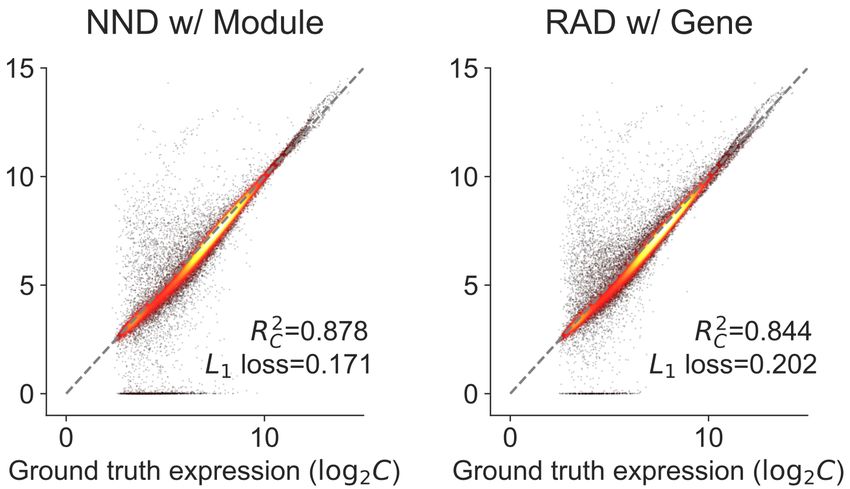
2                                                                                                                                                     Tao et al.

     Cancers develop through a process of clonal evolution, in which               simulated and real datasets. Biologically, we applied the RAD algorithm
populations of genetically distinct tumor cells evolve and adapt                   to transcriptomic data from matched breast cancer primary and metastatic
functionally coordinate with interaction with various non-cancerous                samples (Priedigkeit et al., 2017b,a; Basudan et al., 2019; Zhu et al., 2019),
stromal cell populations (Beerenwinkel et al., 2016). Metastasis occurs            extending our prior analysis of brain metastasis specifically (Tao et al.,
when a population of tumor cells escape normal controls on cell growth,            2019b) to consider variations across multiple metastatic sites. We further
migrate to a distant site, and successfully establish themselves in that site      applied a refined phylogeny inference algorithm to trace the evolutionary
and continue to develop (Riihimäki et al., 2018). Because of its medical           trajectories from the primary tumor to different metastatic sites (Tao et al.,
importance, the metastatic transition has been the focus of intensive prior        2019b). Our analysis showed that although the breast tumors of different
study (Nguyen et al., 2009). It is particularly important to understand this       metastatic types encompass heterogeneous and distinct cell populations,
process at a clonal level if we wish to identify those tumors at particular risk   there exist common patterns of perturbed pathways detected at the early
for metastasis and find markers and potential therapeutic targets specific         stage of primary breast cancer, suggesting that our framework might shed
to their metastatic clones (Tao et al., 2019a).                                    light on early diagnostic and treatment options.
     Previous research has revealed multiple recurrent features common
to breast cancer metastasis, such as dramatic perturbations in the PI3K-
Akt, RET, and ErbB pathways based on the paired transcriptome of breast            2 Materials and methods
primary and brain metastatic sites (Priedigkeit et al., 2017b; Vareslija et al.,   2.1 Overview
2018). Methods for tumor phylogenetics (Schwartz and Schäffer, 2017),
                                                                                   Figure 1 illustrates the general approach for unmixing bulk RNA from
i.e., inference of evolutionary trees on tumor cell populations, have proven
                                                                                   paired breast cancer metastatic samples and inferring underlying tumor
powerful for characterizing genomics of progression processes, including
                                                                                   evolutionary processes. To reduce the noise of bulk RNA, we first compress
in metastatic progression. Past research has shown that deconvolution
                                                                                   the expression levels of individual genes into the modules using external
and phylogenetic methods allow one to infer evolutionary trajectories in
                                                                                   knowledge bases (Fig. 1a; Sec. 2.2.2). We then apply a novel robust and
breast cancer brain metastases from either bulk genomic or transcriptomic
                                                                                   accurate deconvolution algorithm to unmix the compressed expression
alterations (Brastianos et al., 2015; Körber et al., 2019; Tao et al., 2019b).
                                                                                   data into expression profiles and fractions of individual cell communities
However, much remains unknown, including whether one can reliably
                                                                                   (Fig. 1b; Sec. 2.2). Finally, we infer the evolutionary trajectories of the
identify those clones most susceptible to metastasis and whether the pre-
                                                                                   unmixed tumor communities. We then analyze perturbed biomarkers, such
metastatic genomics of these clones or their subsequent evolutionary
                                                                                   as activity of cancer-related regulatory pathways, during tumor metastasis
trajectories influence their eventual metastatic sites (brain, ovary, bone,
                                                                                   (Fig. 1c; Sec. 2.3).
and gastrointestinal tract).
                                                                                       Note that our overall goal is to deconvolve tumor cell communities (Tao
     Much of the current advances in tumor phylogenetics are coming
                                                                                   et al., 2019b), as opposed to necessarily single cells, and describe their
from single-cell sequencing technologies, such as single-cell RNA-
                                                                                   evolution across the metastatic transition. A cell community is defined as
Seq (scRNA) and single-cell DNA-Seq (scDNA), which allow one to
                                                                                   one or more cell types with potentially distinct expression profiles that
characterize clonal heterogeneity with precision (Navin, 2015). In practice,
                                                                                   share common mixture proportions across samples, indicative of their
though, these kinds of data are rarely available for matched primary and
                                                                                   possible interaction or co-association in the tumor. For example, a set
metastatic samples. Such studies depend on analyzing paired samples
                                                                                   of immunogenic tumor clones and the immune cell types infiltrating them
generally gathered years apart, where primary tumors are generally
                                                                                   may form a community exhibiting an overall expression pattern that is a
archived and no longer amenable to single-cell analysis. While rapid
                                                                                   mixture of those of its constituent cell types. Although our deconvolution
autopsy studies (Alsop et al., 2016) are beginning to recruit cohorts in
                                                                                   algorithm can identify correct numbers of distinct clones when they are
which data can be gathered promptly at both initial diagnosis and mortality,
                                                                                   mixed in distinct proportions in different samples (Sec. 3.2), it is more
the difficulty of recruiting subjects and cost of gathering comprehensive
                                                                                   proper to interpret results as describing cell communities when the sample
single-cell data makes it still prohibitive to gather paired single-cell data
                                                                                   size is small or when tumor cells may associate or coevolve with their
for reasonable sizes of study cohort. In contrast, matched bulk data,
                                                                                   stroma (Beerenwinkel et al., 2016).
e.g., RNA-Seq of both breast primary and metastatic samples, are easier
to acquire when one or both samples have been archived (Zhu et al.,
2019). Inferring clonal evolution from paired archived samples is thus             2.2 RAD: Toolkit for robust and accurate deconvolution
still dependent on an older class of method that sought to study cancer at
                                                                                   We proposed and developed the toolkit called Robust and Accurate
the clonal level through deconvolution (unmixing) of genomic data from
                                                                                   Deconvolution: RAD. RAD is a set of tools that solves the problem of 1)
bulk samples (Beerenwinkel et al., 2005).
                                                                                   estimating the number of cell communities from bulk RNA, 2) unmixing
     Here we build on our past work in developing deconvolution
                                                                                   the cell communities from bulk data, and 3) inferring other biomarkers
methods for understanding the metastatic transition (Tao et al., 2019b).
                                                                                   such as pathways from the deconvolved communities. Table 1 shows an
Our contributions in the present work are two-fold. Methodologically,
                                                                                   example of applying RAD to a common RNA deconvolution problem.
we proposed and developed a tool kit called Robust and Accurate
Deconvolution (RAD), the core algorithm of which takes bulk RNA as
input, and infers the expressions and proportions of groups of associated          Table 1. Functions in the RAD package. The five-line demo shows a
tumor cells, which we denote cell communities. We refer readers to                 typical application of RAD package, which takes as input the bulk RNA
Sec. 2.2 and Sec. 3.3 for the major novelty and advancement of RAD,                data B, bulk marker data BP , and gene module knowledge, and outputs
and the differences between RAD and previous deconvolution algorithms              deconvolved RNA C, biomarker CP , and fractions F.
such as NMF (Lee and Seung, 2000), Geometric Unmixing (Schwartz                            Function                              Demo code
and Shackney, 2010), LinSeed (Zaitsev et al., 2019), and NND (Tao                   compress_module             B_M     =   compress_module(B, module)
et al., 2019b). We show that RAD can automatically identify correct                 estimate_number               k     =   estimate_number(B_M)
numbers of cell populations and identify perturbed biomarkers, such                 estimate_clones          C_M, F     =   estimate_clones(B_M, k)
                                                                                    estimate_marker             C_P     =   estimate_marker(B_P, F)
as cancer pathways. We validated its superiority over alternative                                                 C     =   estimate_marker(B, F)
deconvolution algorithms through comprehensive validations on both
Robust and accurate deconvolution of tumor populations in breast cancer metastasis                                                                              3

                                      a   Module 1                  b                                          c
                                                                                       or      or      ?

                         Cancer                                         100%
                         biology
                                                         Module 3

                                          Module 2
                                                                         0%
                                                                                breast brain   ovary   bone

                      Computational
                         model                                      ≈                  ×

Fig. 1: Illustration of discovering underlying cancer evolutionary mechanisms of metastatic progression using the proposed computational models.
(a) Gene module compression. Genes from the same modules have similar co-expression patterns. By mapping the individual genes into modules, we can
get a cleaner representation of bulk RNA data. (b) Deconvolution of bulk RNA. Using the RAD algorithm, we unmixed the bulk data into two matrices:
expression matrix and fraction matrix, which represent the expression profile and fractions of individual cell populations. (c) Phylogeny inference of cell
communities. The inferred phylogeny represents the most likely evolutionary trajectories of cell populations.

    RAD is different from the traditional non-negative matrix factorization          warm-start procedure to develop an initial guess as to a solution, coordinate
(NMF; Lee and Seung 2000) widely used in this problem domain. First,                 descent optimization to improve fit to the objective, and a minimum
RAD considers a biologically meaningful unmixing problem (Sec. 2.2.1),               similarity selection procedure to identify the most informative partitioning
which has additional constraints that make it much harder to solve than              among a set of random restarts — as described in more detail below.
the general NMF problem. Although there exist many NMF variants
that consider different regularizations, such as NMF with `1 -norm (Shen             2.2.2 Knowledge-driven gene module compression
et al., 2014) and sparseness (Hoyer, 2004), these NMF algorithms                     By default, RAD unmixes the raw expression matrix C directly. However,
mainly consider the prior of data distribution instead of the biological             gene module compression (compress_module) is a suggested option if
feasibility. As far as we know, the only algorithm that solves this specific         we have prior information on what genes belong to the same gene modules.
deconvolution problem is our gradient descent-based NND method (Tao                  Gene expressions within the same gene modules are highly correlated,
et al., 2019b). Algorithms derived from the widely used multiplicative               which can be explained by their shared genomic context, similar biological
update (MU) rules do not necessarily guarantee the convergence or                    functions, or participation in the same interaction network (Tao et al.,
accuracy in this new scenario (Lei et al., 2020a,b), a problem that RAD              2020). Intuitively, we can compress the noisy expressions of individual
tackles by using a hybrid solver. Second, NMF is fragile since the unmixed           genes into cleaner “gene modules” (Desmedt et al., 2008; Park et al.,
matrices may be distinct given a different initialization seed. In contrast,         2009), to reduce the signal-to-noise ratio (SNR).
RAD employs both the prior knowledge of gene modules and the minimum                      Here we utilize the functional annotation clustering tool in DAVID
similarity criteria to generate robust and reliable output. Lastly, RAD is           to group the top 3,000 most varied genes into around 100 to 200
a toolkit that aims to resolve a series of problems in the deconvolution of          modules (Huang et al., 2009), where multiple external knowledge
bulk RNA, while NMF mainly focuses on optimizing the objective function              databases are used to facilitate the clustering. The gene expressions within
efficiently.                                                                         the same module are averaged to get the module expression value. The
                                                                                                                                                 1 ×n
                                                                                     resulting bulk compressed module matrix is BM ∈ Rm        +      , where m1
2.2.1 Deconvolution problem formulation                                              is the total number of modules.
Given a non-negative bulk RNA-Seq expression matrix B ∈ Rm×n       +       ,              The gene module compression in our work is knowledge-driven,
where each row i is a gene, each column j is a tumor sample, our goal is to          which is reliable even when only limited tumor samples are available,
infer an expression profile matrix C ∈ Rm×k
                                         +      , where each column l is a           in contrast to prior work using data-driven clustering of coexpressed
cell community, and a fraction matrix F ∈ Rk×n
                                             +   , such that: B ≈ CF.                genes (Zaitsev et al., 2019), which is more dependent on large sample
To be more concrete, we formulated the problem, as in our prior work (Tao            sizes. We validate the superiority of knowledge-driven compression over
et al., 2019b), as follows:                                                          data-driven compression on a real dataset (Fig. 4b,e), and the effect of such
        min kB − CFk2Fr ,                                                 (1)        knowledge-driven compression (Fig. 4d,e) in Sec. 3.3.
        C,F

          s.t. Cil ≥ 0,      i = 1, ..., m, l = 1, ..., k,                (2)        2.2.3 Core algorithm of RAD
                                                                                     The core algorithm of RAD (estimate_clones) unmixes the
               Flj ≥ 0,      l = 1, ..., k, j = 1, ..., n,                (3)
                                                                                     compressed bulk RNA data BM into expression profiles CM and
               Xk
                         Flj = 1,             j = 1, ..., n,              (4)        fractions F of individual communities. The method works in three phases
                   l=1
                                                                                     – warm-start, coordinate descent, and minimum similarity selection – to
where kXkFr is the Frobenius norm. The column-wise normalization of
                                                                                     achieve accuracy and robustness. RAD can directly unmix the original
Eq. (4) ensures that the total fractions of all cell communities in the same
                                                                                     bulk RNA data B as well, and we will remove the subscript M in this
sample sum up to one. This optimization problem is non-convex and non-
                                                                                     section for simplicity.
trivial to resolve. In addition, the bulk data B is noisy, so even an optimal
solution does not necessarily fit the ground truth C and F. Our overall              Warm-start – The warm-start phase borrows its idea from the
approach to solve for this problem consists of three phases — a randomized           multiplicative update (MU) rules for the general NMF problem (Lee and
4 Tao et al.
Seung, 2000). It first randomly initializes C and F from the uniform B: M, Mtest ∈ {0, 1}m×n (M is Mtrain . We omit the subscript train
distribution U (0, 1) then iterates the following loop until the objective for simplicity.), and M + Mtest = 1m×n . Bij is blocked when the
function converges: corresponding position of Mij = 0. In each fold, 5% of the Mtest are
C←C (BF| ) (CFF| ) , (5) 1’s, and 95% of the M are 1’s. Note that the positions of the 1’s and 0’s
are randomly distributed across the whole matrices M and Mtest , rather
F←F (C| B) (C| CF) , (6) than column-wise or row-wise.
, k
X At the time of validation, we can calculate the “normalized MSE” as
Flj ← Flj Fl0 j , l = 1, ..., k, j = 1, ..., n, (7) the CV error on validation set:
.
l0 =1
kMtest B − ĈF̂ k22 kMtest Bk22 (14)
where and are element-wise product and element-wise division
operators. We add an additional MU step Eq. (7) to the original two At the time of training, we want to optimize the following objective
MU steps Eq. (5-6) to satisfy the constraint Eq. (4). This deteriorates the function with the same constraints to Eq. (2-4):
convergence guarantee of the original MU rules. Therefore, we have to stop min kM (B − CF)k2Fr . (15)
C,F
the update once the objective stops decreasing. However, the revised MU
There exist corresponding algorithms for MU warm-start and
rules in the warm-start phase still have the advantage of fast convergence
coordinate descent phases when a mask M exists. The MU rules to
even when the initial values of C and F are far from optimal solution, and
optimize the masked objective Eq. (15) is similar to Eq. (5-7). However,
can provide a reasonable starting point for the second phase.
Eq. (5,6) are revised to the following rules:
Coordinate descent – After the warm-start phase, the coordinate descent C←C ((M B) F| ) ((M (CF)) F| ) , (16)
phase optimizes over the two coordinates C and F iteratively until the
| |
objective function converges: F←F (C (M B)) (C (M (CF))) . (17)
C ← arg min kB − CFk2Fr , (8) The coordinate descent iterations of the masked version are the same to
C the unmasked version Eq. (8-12), except that (B − CF) in Eq. (8,10) are
s.t. Cil ≥ 0, i = 1, ..., m, l = 1, ..., k, (9) replaced with M (B − CF). The sub-problems of the two masked
and coordinate descent steps are still quadratic programming problems.
F ← arg min kB − CFk2Fr , (10)
F 2.2.5 Cancer-related pathway annotation
We further processed the bulk data to derive aggregate biomarkers profiling
s.t. Flj ≥ 0, l = 1, ..., k, j = 1, ..., n, (11)
activity of cancer-related pathways. Although this is not part of the RAD
Xk
Flj = 1, j = 1, ..., n, (12) toolkit, we make use of bulk biomarkers and estimates of their activity in
l=1
individual cell components (Sec. 2.2.6) to interpret the results of the RAD.
Although the original optimization problem Eq. (1-4) is non-convex,
We extracted 24 cancer-related pathways and the corresponding genes
the two sub-problems of the coordinate descent are convex and can be
from the pathways in cancer (hsa05200), breast cancer (hsa05224), and
solved using general quadratic programming. We used the Python package
glioma (hsa05214) of the KEGG database (Kanehisa and Goto, 2000). The
cvxopt (Andersen et al., 2013). The coordinate descent phase can
value of each pathway is the average expression of all genes within it. We
usually further reduce the loss function by around 5% to 30% after the
mapped the original bulk gene matrix B into the cancer pathway probes
warm-start phase, as evaluated on a real dataset GSE19830 (Sec. 2.5.2;
matrix BP ∈ R24×n + . Readers can find the list of pathways in Fig. 5.
Shen-Orr et al. 2010).
Cancer pathways are distinct from gene modules, which capture
Minimum similarity selection – Since the deconvolution problem Eq. (1-4) the major variance across samples and the co-expression patterns using
is non-convex, different initialization values of C and F may converge to prior knowledge to facilitate more reliable deconvolution. However, co-
distinct solutions. We reran the initialization, warm-start, and coordinate expression modules are often weakly linked to biological functions and
descent for multiple times (10 in our experiments) and selected the not informative for downstream analysis. In contrast, biomarkers such as
solution with minimum similarity of expression profiles. We defined the cancer-related pathways facilitate functional interpretation of results. We
unnormalized cosine similarity of a specific solution C as: did not use cancer-related pathways or other biomarkers for deconvolution,
k−1 k since they are not representative of the expression profiles.
C|·l C·l0 .
X X
cosim(C) = (13)
l=1 l0 =l+1 2.2.6 Pathway estimation of cell communities
Biologically, the use of minimum similarity is motivated by the assumption Given the bulk cancer pathway data BP , RAD utilizes the
that individual cell communities should be distinct from each other. deconvolved F to infer the pathway values of cell populations CP
Minimum similarity performs slightly better than minimum loss on (estimate_marker), similar to the paradigm of the Digital Sorting
GSE19830 dataset, although the two criteria often overlap empirically. Algorithm (DSA; Zhong et al. 2013), by replacing B and C with BP and
CP in Eq. (8,9). The unmixed C or CM may not be easy to interpret.
However, other biomarkers, such as cancer pathways, provide a possible
2.2.4 Estimating number of communities
way to explain the biological process of each cell community, and can
The core algorithm of RAD infers the C and F from B given a specific
be used as input to infer the phylogeny and perturbed pathways during
number of communities k, which in practice is unknown to us in advance.
progression (Sec. 2.3).
RAD estimates the number of cell components (estimate_number)
through cross-validation (CV). The estimated/optimal k reflects the trade-
off between model bias and the variance.
2.3 Phylogeny inference through minimum elastic potential
We take a 20-fold CV as an example: In each fold, 5% of the elements Given the deconvolved cell clone profiles C ∈ Rn×k + of k cell
in B are unseen at the time of training/optimization. At the time of test, components, we inferred trees describing the observed extant and
the loss is calculated only on these unseen 5% elements. Technically, unobserved ancestral Steiner communities. We use the term “phylogeny”
we realized it by utilizing the mask matrices with the same shape of to refer to these trees to highlight their connection to tumor phylogeneticsRobust and accurate deconvolution of tumor populations in breast cancer metastasis 5
methods often used for similar purposes and on similar data (Schwartz and We considered the expression of 2,048 interested genes and assumed
Schäffer, 2017), although we recognize that these trees describe changes in three pure cell clones C ∈ R2048×3
+ . In the case where each module
mean transcriptomic states of groups of associated cells rather than strictly consists of just one gene, C was drawn from a log-normal distribution
clonal evolution and thus are not proper phylogenies. independently (Bengtsson et al., 2005):
RAD works in the original non-log linear space, which recovers
Cil ∼ 2N (6,2.5 ) ,
2
i = 1, 2, ..., 2048, l = 1, 2, 3. (19)
underlying components with higher accuracy and lower bias (Zhong
and Liu, 2012). In the phylogeny inference algorithm, however, we We assumed that genes from the same module are highly correlated and
instead used the log space to focus on the fold change of expressions prone to co-express. When module size is greater than one, e.g., there are
4×3
C ← log2 (C + 1). We also normalize the expression to make them four genes in a module, for each gene module CS ∈ R+ (a subblock
have zero mean value for each gene. of C), we draw each gene module as follows:
| ,2.52 Σ
We used a variant of the minimum elastic potential (MEP) method to (CS )·l ∼ 2N ([6,6,6,6] ), l = 1, 2, 3, (20)
infer the phylogeny structure and expression values of Steiner nodes (Tao where Σ is the covariance matrix of four genes in the module:
et al., 2019b). Taking C as input, the MEP first builds the phylogeny
1 0.95 0.95 0.95
tree that includes k extant nodes and (k − 2) ancestral Steiner nodes 0.95 1 0.95 0.95
using the neighbor-joining (NJ) algorithm (Nei and Saitou, 1987). To Σ= . (21)
0.95 0.95 1 0.95
identify the perturbed biological processes and gene expression during
0.95 0.95 0.95 1
tumor evolution, MEP infers expression values of the unknown Steiner
nodes by minimizing an “elastic potential energy”. For a specific pathway We assumed 100 mixture samples of bulk RNA, and drew the fractions
or gene, this is equivalent to a quadratic programming problem: of mixture samples uniformly from a unit simplex:
1 | F·j ∼ U [∆3 ], j = 1, 2, ..., 100, (22)
min x P(W)x + q(W, y)| x, (18)
x 2 Finally, we added the noise of magnitude σ to get the final bulk data:
where x ∈ Rk−2 , y ∈ Rk are the expression values of Steiner and
Bij ∼ (CF)ij + 2N (0,σ ) , i = 1, 2, ..., 2048, j = 1, 2, ..., 100.
2
extant nodes; P(W) is a function that takes as input the tree edge weights
(23)
W and outputs a matrix P ∈ R(k−2)×(k−2) ; q(W, y) is a function
that takes as input edge weights W and vector y and outputs a vector
2.5.2 GSE19830 dataset
q ∈ Rk−2 . We further added an `2 -regularization λI(k−2)×(k−2) to
GSE19830 contains RMA-normalized Affymetrix expressions of cells
the P(W). In practice we use λ = 0.001, which helps more stable
from rat brain, liver, and lung biospecimens (Shen-Orr et al., 2010). It
inference when the total number of nodes is large. Interested readers can
mixed the three pure tissues in different predefined proportions, leading to
find detailed problem formulation, derivatives, and proofs of MEP in the
33 mixture samples. Expression profiles of each pure and mixed sample
previous work (Tao et al., 2019b).
were measured three times.
Although we used the notation C for the explanation in this section,
We removed the non-protein coding genes, conducted quantile
in our application, we used the pathway probes CP to infer the cancer
normalization, and took the average of three replicates. This yielded three
pathway values of each Steiner nodes for downstream interpretation.
matrices for the GSE19830 data: expression profiles of the three pure
clones C ∈ R13741×3
+ , fractions of three clones in all mixture data
2.4 Evaluation F ∈ R3×33
+ , and bulk data B ∈ R13741×33
+ .
The deconvolution algorithm outputs both the estimated expression
profiles Ĉ and the fractions F̂ of each cell communities. We utilized four 2.5.3 BrM dataset
different metrics to measure the accuracy and error of the two estimators The BrM dataset contains matched transcriptome data of breast cancer
with the ground truth C and F following previous research (Zaitsev et al., metastasis patients (Zhu et al., 2019). There are 102 samples from 51
2019; Zhu et al., 2018; Newman et al., 2015): RC 2
(Pearson coefficient of patients in total. There are four possible different metastatic sites for each
2
Ĉ and C), L1 loss (kĈ − Ck1 /kCk1 ), RF (Pearson coefficient of F̂ breast cancer patient in the dataset: brain (BR; 22 patients), ovary (OV; 13
and F), MSE (Mean square error of F̂ and F). patients), bone (BO; 11 patients), and gastrointestinal tract (GI; 5 patients).
A sample from the primary breast site has a matched sample from the
metastatic site of the same patients. RNA-Seq of around 60,000 genes
2.5 Datasets and preprocessing are available. We will denote the sample from the metastatic site and
We utilized three datasets throughout this work: one real dataset of breast the corresponding primary site as MBR/PBR, MOV/POV, MBO/PBO,
cancer metastasis (BrM; Zhu et al. 2019); one real dataset of both pure MGI/PGI. We removed the non-protein coding genes and conducted
19689×102
and mixed transcriptome of liver, brain, and lung (GSE19830; Shen-Orr quantile normalization to get the final bulk data: B ∈ R+ .
et al. 2010); and one simulated dataset. All three datasets contain bulk
transcriptome B, which is the input of RAD and downstream analysis.
3 Results
Ground truth C, F are only available in simulated and GSE19830 datasets,
and unknown in BrM dataset. Ground truth module knowledge of genes are 3.1 Gene modules facilitate robust deconvolution
only available in simulated dataset, GSE19830 and BrM datasets instead RAD can act directly on the bulk gene expression B or on the knowledge-
used DAVID to infer gene module. based compressed bulk gene module expression BM (Sec. 2.2.2). We
validated that the gene module compression is beneficial to RAD through
2.5.1 Simulated dataset both simulated data and real datasets.
We simulated a series of datasets with different parameters of module size As a proof of concept, we first assume the knowledge of gene modules
(1, 2, 4, ..., 512) and noise level σ ∈ [0, 5] to validate the effectiveness is correct and known to us. We generated simulated bulk data with a noise
of RAD and module compression. We selected most of the parameters level σ = 4 and various module sizes from 1 to 512 (Sec. 2.5.1). We
following Zaitsev et al. (2019), with selected parameters consistent with calculated four metrics to evaluate the accuracy of RAD estimation on
the distribution of the real dataset GSE19830. these data, and repeated all experiments 100 times (Fig. 2). A moderate6 Tao et al.
a b from one to three, and flattens after k goes over three. In this case, we
identify the correct number of cell clones to be three1 .
For the BrM dataset, we applied a 20-fold CV as well and found the CV
error drops when k is smaller than seven, and increases with substantial
variance because of overfitting when k is higher than seven. We therefore
used k=7 as the number of communities in the BrM data. Previous research
using a subset of the BrM dataset (only breast cancer brain metastasis
c d samples) identified only five cell populations (Tao et al., 2019b). With a
larger sample size, and more heterogeneous data, we can identify more
fine-grained unmixed cell communities.
3.3 RAD estimates cell populations robustly and accurately
We then evaluated the accuracy and error of RAD relative to alternative
deconvolution algorithms. There are many algorithms to solve the “partial
Fig. 2: Effectiveness of gene module representation. Compressing the
deconvolution” problem, where the expression profiles of clones C are
expression of individual genes into gene modules can promote more robust
available at the time of deconvolution, e.g., DSA (Zhong et al., 2013).
deconvolution with proper module size. We tested on the simulated bulk
For tumor samples, however, the underlying cell types are often unknown,
data with the noise level of σ = 4, and repeated all the experiments for
and partial deconvolution can be unstable. We consider the “complete
100 times to get the boxplot. We evaluated four metrics that measure the
deconvolution” problem here (Zaitsev et al., 2019), where the expression
accuracy of deconvolution with different gene module sizes. Note that
profiles of populations C are not available and must be inferred.
“module size” of one is equivalent to the original gene expression without
2
There are a few existing algorithms that seem to be suitable for the
module compression. (a) Accuracy of expression matrix estimation: RC .
complete deconvolution problem, e.g., principal components analysis
(b) Error of expression matrix estimation: L1 loss. (c) Accuracy of fraction
2
(PCA), independent components analysis (ICA), and NMF. However, none
matrix estimation: RF . (d) Error of fraction matrix estimation: MSE.
of these algorithms account for the fraction normalization constraints
a b Eq. (4), and PCA and ICA do not guarantee the non-negativity of
expression profiles Eq. (2). A few more well-designed algorithms have
been developed for the specific complete deconvolution problem, including
Geometric Unmixing (Schwartz and Shackney, 2010), LinSeed (Zaitsev
et al., 2019), and NND (Tao et al., 2019b):
• Geometric Unmixing: It poses unmixing as a problem from
computational geometry by assuming all the bulk samples are located
in a simplex, where the corners of the simplex represent the expression
Fig. 3: Cross-validation to automatically select the number of cell profiles of pure clones.
communities. We conducted a 20-fold cross-validation to infer the optimal • LinSeed: Based on the observation that genes in the same module
number of cell component k as the input of RAD algorithm. (a) Cross- are highly correlated to each other. It first identifies these anchor
validation on GSE19830 dataset. The actual number of cell clones is genes through linear correlation. Then it uses a partial deconvolution
three. (b) Cross-validation on BrM dataset. The inferred number of cell algorithm DSA to infer the fractions F and expressions of non-anchor
components is seven, which is used as the input parameter for Fig. 5-7. genes C (Zhong et al., 2013).
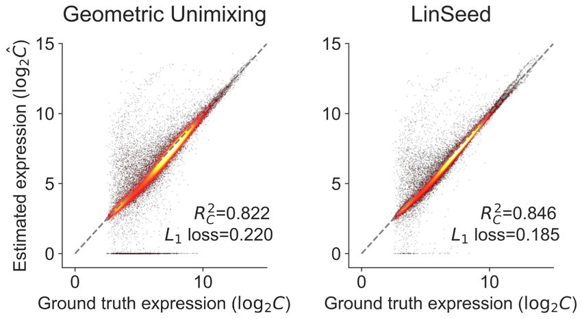
• NND: It converts the complete deconvolution problem equivalently
module size of 32 makes RAD the most accurate (highest median accuracy) into an optimization problem, which can be implemented as a neural
and robust (smallest variance), which is helpful to deconvolution. RAD is network. It uses backpropagation (gradient descent) to optimize.
less robust (high variance) on the original uncompressed bulk gene data
For RAD, we can directly take as input the bulk gene expression matrix
(module size of one). However, when module size is too large, RAD has
both inaccurate and unstable performance. We refer interested readers to
B (Fig. 4d), or use the more noise-free bulk module expression matrix BM
(Fig. 4e). Although the NND can also take B or BM in principle, we only
Fig. S1 for a more comprehensive results on the effects of both module
included results of “NND w/ Module” (Fig. 4c), due to the intractable
size and noise level on RAD performance.
training time of “NND w/ Gene”.
We further examined whether the module knowledge from DAVID
Figure 4 compares the performance of the five deconvolution
generates a reasonable module size and facilitates robust RAD
algorithms and module-compressed variants on the GSE19830 dataset.
deconvolution. We applied RAD to both the uncompressed and compressed
The gene module compression improves the accuracy of RAD significantly
GSE19830 dataset. As one can see in Fig. 4d,e, module compression based
(Fig. 4d,e), consistent with the observations in Fig. 2. The RAD on the
on DAVID improve the RAD estimation of both C and F.
compressed module data outperforms the other three algorithms in metrics
We could not directly validate the effectiveness of DAVID compression 2 2
on unmixing the BrM dataset, but we found the gene module representation
RC , RF , and MSE (Fig. 4a-c,e). It also has comparable L1 loss with
the “NND w/ Module” algorithm (Fig. 4c,e). These results reveal the
informative for separating primary and metastatic samples (Fig. S2).
superiority and accuracy of the RAD algorithm and module compression.
The elevated accuracy and robustness of RAD over competing
3.2 RAD detects the correct number of cell components algorithms is crucial for downstream analyses such as phylogeny inference.
RAD utilizes cross-validation (CV) to identify the number of underlying For example, RAD reveals a more detailed portrait of perturbed pathways
cell populations (Sec. 2.2.4). To validate its correctness, we applied a 20-
fold CV to the GSE19830 data. As one can see in Fig. 3a, the CV error 1 Although k=8 gives minimum CV error, it is due to the small noise or
Eq. (14) drops quickly when the number of cell components k increases artifacts in the samples.Robust and accurate deconvolution of tumor populations in breast cancer metastasis 7
a b c d e
Fig. 4: Performance of different deconvolution algorithms on GSE19830 dataset. We compared the accuracy of both estimated C and F across four
2 2
different deconvolution algorithms. RAD with the module achieves best the performance among all the deconvolution algorithms evaluated in RC , RF ,
and MSE. The module information facilitates the RAD to achieve better performance. (a) Geometric Unmixing. (b) LinSeed. (c) NND (with module).
(d) RAD (with gene). (e) RAD (with module).
Pathway strength
10.5 12.2 10.5 0.0 0.0 9.0 8.6 ErbB signaling pathway a C6 b C6
11.4 12.5 11.0 0.4 9.7 9.4 11.3 ↓ ECM-receptor
Estrogen signaling pathway ↓ PI3K-Akt
↓ ECM-receptor
↓ PI3K-Akt
13.8 13.7 10.7 11.1 0.1 16.6 5.6 ECM-receptor interaction ↓ Focal adhesion ↓ Focal adhesion
↓ Hedgehog ↑ Estrogen
12.8 14.8 10.4 11.8 0.1 15.3 11.1 Focal adhesion ↑ Apoptosis
12.1 12.2 10.0 9.0 0.0 14.5 9.0 ↓ Hedgehog
PI3K-Akt signaling pathway ↓ RET
S1 ↓ ECM-receptor
S2 ↓ RET
11.7 15.9 11.5 12.8 1.1 10.8 12.5 Adherens junction ↓ Cytokine receptor ↓ Focal adhesion ↑ RET ↓ Hedgehog
↑ Adherens junction ↑ RET ↓ ECM-receptor
10.3 11.4 10.0 6.6 4.5 9.8 10.1 MAPK signaling pathway ↑ Apoptosis ↓ PI3K-Akt ↓ Cytokine receptor
9.2 11.4 9.6 8.3 0.0 9.2 9.0 Calcium signaling pathway
C2 S3 ↓ Focal adhesion C1 ↓ Hedgehog S1 ↓ ECM-receptor
11.4 12.6 10.8 9.0 0.0 10.1 10.9 HIF-1 signaling pathway ↓ Cytokine receptor ↓ Focal adhesion
↓ Adherens junction ↓ PI3K-Akt
10.6 12.9 11.3 10.6 0.0 9.3 10.5 ↓ RET
PPAR signaling pathway ↑ RET ↓ HIF-1
↑ Adherens junction ↓ Adherens junction
↓ PI3K-Akt ↓ HIF-1
8.5 0.0 11.2 10.0 0.0 5.3 10.2 RET ↓ PPAR
↑ Apoptosis
6.4 0.0 6.4 7.0 5.9 6.9 6.5 ↑ RET C2 C5
Cytokine-cytokine receptor interaction ↑ ECM-receptor S2 C5
8.8 0.0 8.2 9.3 8.5 8.7 9.0 Hedgehog signaling pathway ↑ ErbB
↓ Apoptosis
9.3 15.0 9.6 12.1 10.3 9.3 11.7 Apoptosis ↓ VEGF ↓ ECM-receptor
9.2 9.4 9.4 10.8 11.2 10.4 10.0 ↑ RET
Notch signaling pathway
8.3 10.4 7.4 7.2 9.2 8.2 9.2 VEGF signaling pathway C3 C7
9.1 5.9 8.1 8.2 8.4 8.0 7.9 Homologous recombination
9.7 9.3 8.9 8.8 9.6 8.4 8.7 Cell cycle
9.0 9.8 9.3 9.2 9.1 9.0 8.4 cAMP signaling pathway c C6 d C6
↓ ECM-receptor
↓ ECM-receptor
9.1 8.1 8.6 9.2 8.8 8.6 8.9 JAK-STAT signaling pathway ↓ Focal adhesion ↓ PI3K-Akt
↓ PI3K-Akt ↓ Focal adhesion
9.1 7.8 8.7 8.8 8.9 8.9 8.0 Wnt signaling pathway ↓ Hedgehog
↑ RET
8.7 7.8 8.6 8.7 8.8 8.6 8.5 mTOR signaling pathway ↓ Cytokine receptor
9.0 8.1 8.7 8.8 7.4 9.7 8.4 S1 ↑ RET S1 ↓ Hedgehog
p53 signaling pathway ↓ ECM-receptor ↓ RET
9.3 7.9 8.9 10.2 8.7 10.3 8.6 ↓ ECM-receptor
TGF-beta signaling pathway ↑ Estrogen
↓ PI3K-Akt ↓ Focal adhesion ↓ Cytokine receptor
↓ PI3K-Akt ↑ Apoptosis
C1 C2 C3 C4 C5 C6 C7 ↑ Hedgehog ↑ Adherens junction
Fig. 5: Cancer-related pathway strengths of each cell component from C1 ↓ ErbB
↓ Estrogen
S2 ↑ RET
↑ ErbB
C3 C2
↓ PI3K-Akt ↓ ECM-receptor
BrM dataset. The strengths are shown in log-scale log2 (CP + 1). ↓ ECM-receptor ↓ Focal adhesion
↓ MAPK ↑ Estrogen
↓ Estrogen S3 ↓ ECM-receptor C3
↓ ErbB ↓ Focal adhesion
PBR POV PBO PGI ↑ Adherens junction ↓ Adherens junction
MBR MOV MBO MGI ↑ RET
↑ Apoptosis
↓ PPAR
↓ PI3K-Akt
C4 C5
0.6
Fig. 7: Phylogenies of four different metastatic cases. Although there
Proportion
0.4
are large differences in tumor communities across the four metastasis sites,
there exists common mechanisms, such as the early events of perturbed
0.2
PI3K-Akt, ECM-receptor, and focal adhesion pathways. (a) Breast cancer
brain metastasis. (b) Breast cancer ovary metastasis. (c) Breast cancer
0.0 bone metastasis. (d) Breast cancer GI metastasis.
C1 C2 C3 C4 C5 C6 C7
Component
Fig. 6: Fractions of communities in both primary and metastatic sites
of four different metastasis types from BrM dataset. The differences 3.4 Landscape of tumor cell communities
of cell distribution exist both between primary (lighter) and metastatic We derived the fractions of cell communities in each sample F using
(darker) sites, and across four metastatic cases (different colors). RAD, and further inferred the pathway values of each cell community from
BP and F (Sec. 2.2.6). Although there exists inter-tumor heterogeneity
across cancer samples, RAD aims to separate the shared features of cell
(Sec. 3.5) during metastasis than our previous NND algorithm (Tao et al., populations across these tumors from sample-specific features as in prior
2019b). cross-cohort deconvolutional phylogeny studies (Schwartz and Shackney,8 Tao et al.
2010; Roman et al., 2015) and prior oncogenetic tree methods that do not There are also substantial differences across metastatic sites that
include a deconvolution step (Desper et al., 2004; Riester et al., 2010). may suggest potential markers of incipient site-specific metastasis. The
dysregulation of some perturbed pathways have already been shown to
Expression profiles of cell communities Figure 5 shows the pathway values
be closely related to tumor progression (Hedgehog, Apoptosis; Gupta
of each cell population in log scale log2 (CP + 1) after applying RAD
et al. 2010). RET and ErbB have been shown recurrently perturbed in
to the BrM dataset. C5 is the most abnormal community, having lost
metastasis (Priedigkeit et al., 2017b). The reduction of Cytokine-cytokine
half of the pathways completely (almost zero expression), including
receptor may reflect the reduced immune cell recruitment in metastatic
PI3K-Akt, ECM-receptor, and Calcium. Another unusual cell community
samples (Zhu et al., 2019).
is C2, which is specifically enriched in neurotransmitter and calcium
homeostasis functions (Calcium and cAMP; Hofer and Lefkimmiatis
2007). We hypothesize that C2 might reflect a cell community combining
both neural cells and metastatic tumor cells. In contrast, C6, which we 4 Discussion
infer to approximate the primary breast tumor community, has a relatively We developed a tool called RAD for deconvolution of multi-stage
high expression of PI3K-Akt (Brastianos et al., 2015) and immune function transcriptomic data corresponding to primary and metastatic tumor
(Cytokine-cytokine receptor; Zhu et al. 2019). samples. We have shown that RAD can robustly and accurately estimate
the number of cell populations, unmix the cell populations, and infer
Distribution of cell communities Figure 6 shows the distribution of cell
biomarkers from bulk RNA-Seq of tumor samples, while showing
components across different metastatic sites. We classified the tumor sites
improved reliability and accuracy over other deconvolution algorithms on
into eight categories: MBR/PBR, MOV/POV, MBO/PBO, and MGI/PGI
both simulated and real RNA datasets. We applied RAD with gene module
(Sec. 2.5.3). We observe that C6 is always decreased in the metastatic
compression and a phylogeny inference algorithm to bulk transcriptome
samples, from which we infer it may approximate the primary clones and
data collected from matched breast primary and four different metastatic
capture features that distinguish primary clones from metastatic ones in
sites to characterize similarities and variations in tumor clonal populations
general. Other components are increased in specific metastasis types. For
by eventual site of metastasis. Significant perturbations of cancer-related
example, C1 in OV and BO; C2 in BR, OV, and GI; C3 in BR, OV, and GI;
pathways, such as PI3K-Akt, ECM-receptor, and focal adhesion emerge
C4 in BO; C5 in BR, OV, and BO; and C7 in BR. This indicates that there
as common early events across sites of breast cancer metastasis, showing
exist different cell population mixtures in different metastatic sites, likely
the potential of the method to reveal recurrent evolution mechanisms of
in part reflecting site-specific stroma but also revealing commonalities
breast cancer metastasis.
across metastatic sites. We further note that the distribution of cell clones
It has been observed that the noise of RNA expression grows with its
across primary sites is related to their eventual sites of metastasis. This
amplitude, suggesting that a more principled probabilistic model instead
result is suggestive that there may be a signal in the primary clonal
of Frobenius norm could potentially further improve the deconvolution
composition of whether a primary tumor is likely to metastasize to a
accuracy (Zhu et al., 2018). Furthermore, we applied RAD by considering
particular site, although that suggestion requires further evaluation and
a limited two-stage progression process, without use of the time-series
validation.
information. One future direction might be extending RAD into a temporal
We do not know the ground truth cell populations in the BrM dataset.
model to take advantage of more precise information on time to metastasis
Given that the component C3 mainly exists in the GI samples (Fig. 6),
when available or more extensive time-series data on multiple time
though, we would predict that removing the GI samples would decrease
points such as might be produced by “liquid biopsy” technologies. We
the optimal number of components from 7 (Fig. 3b) to 6, which is indeed
mainly focused on transcriptome data in this work, but we expect the
the case (Fig. S3).
RAD algorithm to be versatile and potentially applicable to other types
of continuous biological data, such as epigenome and proteome. With
3.5 Common evolutionary mechanisms of breast cancer moderate adaptations, it is also possible to apply RAD to genome data,
metastasis which is one major focus of cancer phylogenetics, such as copy number
variations (Eaton et al., 2018). While much of the motivation for this work
Using the unmixed cell clones CP , we built a phylogeny and inferred
is the difficulty of acquiring scRNA for primary tumor samples when
the pathway values of Steiner nodes using the MEP algorithm (Sec. 2.3).
examining metastases years later, we do anticipate that this problem will
Since there are vast differences across the four metastasis types (Fig. 6), we
lessen over time. It is thus worth considering for the future whether our
inferred a phylogeny tree for each metastasis type (Fig. 7a-d; Table S1-S4).
methods might be adapted for working on limited and noisy scRNA with
We presented C6 as the common root node, as it consistently decreases
matched bulk data (Elyanow et al., 2020).
in all four metastasis types, and identified the communities whose average
fractions increase in the metastatic communities of specific metastasis
types. Figure 7 shows the top five most differentially expressed pathways
for more than one fold along each edge. Acknowledgments
As one can see, there are common patterns at the early stage of We would like to thank to the reviewers for their helpful suggestions.
metastasis, e.g., the decrease of PI3K-Akt, ECM-receptor interaction,
and focal adhesion. The loss of PI3K/Akt/mTOR in metastatic tumors has
already been identified in brain metastasis research based on both genomic
Funding
and transcriptomic data (Brastianos et al., 2015; Tao et al., 2019b). Our
result indicates the loss of PI3K-Akt pathway is a common event among This work is partially supported by NIH awards R21CA216452 and
the general metastasis types as well, not limited to brain metastasis. Loss R01HG010589, Pennsylvania Department of Health award #4100070287,
of ECM-receptor interaction and focal adhesion also plays a critical role Susan G. Komen for the Cure, the Mario Lemieux Foundation, and
in tumor cell migration generically (Nagano et al., 2012). Tumor cells the Breast Cancer Alliance. It is also partially supported by the AWS
adhere to the extracellular matrix (ECM), forming the structures called Machine Learning Research Awards granted to J.M. and R.S., and by the
focal adhesions, and loss of these interactions is a key step in enabling Center for Machine Learning and Health Fellowship granted to Y.T. The
metastatic migration. Pennsylvania Department of Health specifically disclaims responsibility
for any analyses, interpretations or conclusions.Robust and accurate deconvolution of tumor populations in breast cancer metastasis 9
References Navin, N. E. (2015). The first five years of single-cell cancer genomics
Alsop, K. et al. (2016). A community-based model of rapid autopsy in and beyond. Genome research, 25(10), 1499–1507.
end-stage cancer patients. Nature biotechnology, 34(10), 1010–1014. Nei, M. and Saitou, N. (1987). The neighbor-joining method: a new
Andersen, M. S. et al. (2013). CVXOPT: A python package for convex method for reconstructing phylogenetic trees. Molecular Biology and
Evolution, 4(4), 406–425.
optimization, version 1.1.6. Available at cvxopt.org, 54.
Newman, A. M. et al. (2015). Robust enumeration of cell subsets from
Basudan, A. et al. (2019). Frequent ESR1 and CDK Pathway Copy-
Number Alterations in Metastatic Breast Cancer. Molecular cancer tissue expression profiles. Nature methods, 12(5), 453–457.
research : MCR, 17(2), 457–468. Nguyen, D. X. et al. (2009). Metastasis: from dissemination to organ-
Beerenwinkel, N. et al. (2005). Mtreemix: a software package for learning specific colonization. Nature Reviews Cancer, 9(4), 274–284.
and using mixture models of mutagenetic trees. Bioinformatics, 21(9), Park, Y. et al. (2009). Network-based inference of cancer progression from
2106–2107. microarray data. IEEE/ACM Transactions on Computational Biology
Beerenwinkel, N. et al. (2016). Computational cancer biology: an and Bioinformatics, 6(2), 200–212.
evolutionary perspective. PLoS computational biology, 12(2). Priedigkeit, N. et al. (2017a). Exome-capture RNA sequencing of decade-
Bengtsson, M. et al. (2005). Gene expression profiling in single cells old breast cancers and matched decalcified bone metastases. JCI insight,
2(17).
from the pancreatic islets of Langerhans reveals lognormal distribution
Priedigkeit, N. et al. (2017b). Intrinsic subtype switching and acquired
of mRNA levels. Genome research, 15(10), 1388–1392.
Brastianos, P. K. et al. (2015). Genomic characterization of brain ERBB2/HER2 amplifications and mutations in breast cancer brain
metastases reveals branched evolution and potential therapeutic targets. metastases. JAMA oncology, 3(5), 666–671.
Cancer discovery, 5(11), 1164–1177. Riester, M. et al. (2010). A differentiation-based phylogeny of cancer
Desmedt, C. et al. (2008). Biological processes associated with breast subtypes. PLOS Computational Biology, 6(5), e1000777.
cancer clinical outcome depend on the molecular subtypes. Clinical Riihimäki, M. et al. (2018). Clinical landscape of cancer metastases.
Cancer Research, 14(16), 5158–5165. Cancer medicine, 7(11), 5534–5542.
Desper, R. et al. (2004). Tumor classification using phylogenetic methods Roman, T. et al. (2015). A simplicial complex-based approach to unmixing
on expression data. Journal of Theoretical Biology, 228(4), 477–496. tumor progression data. BMC bioinformatics, 16, 254.
Eaton, J. et al. (2018). Deconvolution and phylogeny inference of Schwartz, R. and Schäffer, A. A. (2017). The evolution of tumour
phylogenetics: principles and practice. Nature Reviews Genetics, 18,
structural variations in tumor genomic samples. Bioinformatics, 34(13),
i357—-i365. 213.
Elyanow, R. et al. (2020). netNMF-sc: leveraging gene-gene interactions Schwartz, R. and Shackney, S. E. (2010). Applying unmixing to gene
for imputation and dimensionality reduction in single-cell expression expression data for tumor phylogeny inference. BMC Bioinformatics,
analysis. Genome research, 30(2), 195–204. 11(1), 42.
Guan, X. (2015). Cancer metastases: Challenges and opportunities. Acta Shen, B. et al. (2014). Robust nonnegative matrix factorization via
Pharmaceutica Sinica B, 5(5), 402–418. L1 norm regularization by multiplicative updating rules. In 2014
Gupta, S. et al. (2010). Targeting the Hedgehog pathway in cancer. IEEE International Conference on Image Processing (ICIP), pages
Therapeutic Advances in Medical Oncology, 2(4), 237–250. 5282–5286.
Hofer, A. M. and Lefkimmiatis, K. (2007). Extracellular Calcium and Shen-Orr, S. S. et al. (2010). Cell type-specific gene expression differences
in complex tissues. Nature methods, 7(4), 287–289.
cAMP: Second messengers as “Third Messengers”? Physiology, 22(5),
Tao, Y. et al. (2019a). Improving personalized prediction of cancer
320–327.
Hoyer, P. O. (2004). Non-Negative Matrix Factorization with Sparseness prognoses with clonal evolution models. bioRxiv.
Constraints. J. Mach. Learn. Res., 5, 1457–1469. Tao, Y. et al. (2019b). Phylogenies derived from matched transcriptome
Huang, D. W. et al. (2009). Systematic and integrative analysis of large reveal the evolution of cell populations and temporal order of
gene lists using DAVID bioinformatics resources. Nature Protocols, perturbed pathways in breast cancer brain metastases. In Mathematical
4(1), 44–57. and Computational Oncology, pages 3–28. Springer International
Kanehisa, M. and Goto, S. (2000). KEGG: kyoto encyclopedia of genes Publishing.
and genomes. Nucleic Acids Research, 28(1), 27–30. Tao, Y. et al. (2020). From genome to phenome: Predicting multiple cancer
Körber, V. et al. (2019). Evolutionary trajectories of IDHWT phenotypes based on somatic genomic alterations via the genomic impact
transformer. In Pacific Symposium on Biocomputing, volume 25, pages
glioblastomas reveal a common path of early tumorigenesis instigated
79–90. World Scientific.
years ahead of initial diagnosis. Cancer Cell.
Lee, D. D. and Seung, H. S. (2000). Algorithms for non-negative matrix Vareslija, D. et al. (2018). Transcriptome characterization of matched
factorization. In Proceedings of the 13th International Conference primary breast and brain metastatic tumors to detect novel actionable
on Neural Information Processing Systems, NIPS’00, pages 535–541, targets. Journal of the National Cancer Institute.
Cambridge, MA, USA. MIT Press. Zaitsev, K. et al. (2019). Complete deconvolution of cellular mixtures
Lei, H. et al. (2020a). Tumor copy number deconvolution integrating bulk based on linearity of transcriptional signatures. Nature Communications,
and single-cell sequencing data. Journal of Computational Biology, 10(1), 2209.
27(4), 565–598. Zhong, Y. and Liu, Z. (2012). Gene expression deconvolution in linear
Lei, H. et al. (2020b). Tumor heterogeneity assessed by sequencing and space. Nature Methods, 9(1), 8–9.
Zhong, Y. et al. (2013). Digital sorting of complex tissues for cell type-
fluorescence in situ hybridization (FISH) data. bioRxiv.
specific gene expression profiles. BMC Bioinformatics, 14(1), 89.
Lin, N. U. et al. (2004). CNS metastases in breast cancer. Journal of
Clinical Oncology, 22(17), 3608–3617. Zhu, L. et al. (2018). A unified statistical framework for single cell and bulk
Nagano, M. et al. (2012). Turnover of Focal Adhesions and Cancer Cell rna sequencing data. The annals of applied statistics, 12(1), 609–632.
Migration. International Journal of Cell Biology, 2012, 310616. Zhu, L. et al. (2019). Metastatic breast cancers have reduced immune cell
recruitment but harbor increased macrophages relative to their matched
primary tumors. Journal for ImmunoTherapy of Cancer, 7(1), 265.Robust and accurate deconvolution of tumor populations in breast cancer metastasis 1
Supplementary information
S1 Performance of deconvolution under different module size and noise level
a b
c d
Fig. S1: Deconvolution performance under different module sizes and noise levels. We show the performance by four metrics, which measure the
accuracy of estimated C and F. When the noise level is low, the compressed gene module does not affect the performance much. However, when the
noise level is high (e.g., around four), a proper module size is helpful to achieve better performance. We repeated each experiments for 10 times and took
average values. The figures are shown by applying a linear interpolation to the following grids: module size ∈ {1, 2, 3, 4, 5, 6, 8, ..., 512, 682, 1024},
2
noise ∈ {0, 0.033, 0.067, ..., 1.0}. (a) Accuracy of expression matrix estimation: RC . (b) Error of expression matrix estimation: L1 loss. (c) Accuracy
2
of fraction matrix estimation: RF . (d) Error of fraction matrix estimation: MSE.You can also read