Route optimization for city cleaning vehicle - De Gruyter
←
→
Page content transcription
If your browser does not render page correctly, please read the page content below
Open Eng. 2021; 11:483–498

Research Article

Łukasz Wojciechowski*, Tadeusz Cisowski, and Arkadiusz Małek

Route optimization for city cleaning vehicle
https://doi.org/10.1515/eng-2021-0049                            with maximum profit and minimum financial outlays. This
Received Oct 07, 2020; accepted Jan 03, 2021                     means that the key factor for the efficient functioning of
                                                                 this system are all types of costs. When collecting waste,
Abstract: The basic problem concerning the waste manage-
                                                                 the main operational cost factors are the driver’s working
ment system is work organization, which should be effec-
                                                                 time and the service time of the waste collection vehicle, as
tive with maximum profit and minimum financial outlays.
                                                                 well as the route that the vehicle has to cover [1]. The major
This means that the key factor for the efficient functioning
                                                                 cost factor for waste collection is the working time and the
of this system are all types of costs. When collecting waste,
                                                                 route that the city’s cleaning vehicle has to take [2].
the main operational cost factors are the driver’s working
                                                                      The main components of total costs also include vehi-
time and the service time of the waste collection vehicle, as
                                                                 cle purchase costs and necessary operating costs [3]. The
well as the route that the vehicle has to cover. The article
                                                                 largest of them are related to fuel consumption [4]. They
presents route optimization solution for a vehicle collect-
                                                                 are the main components of the Total Costs of Ownership
ing urban waste (both mixed and segregated) is a simple
                                                                 (TCO) [5]. The cost of purchasing a vehicle usually depends
method of determining the order of driving through individ-
                                                                 on its build quality and the engine unit. In the 21st century,
ual city streets. The prepared solution is universal and is
                                                                 hybrid [6, 7] and electric drives [8, 9] are usually used. This
not limited only to the surveyed housing estate. It presents
                                                                 is evidently due to the advantages they have in relation to
a pattern that can be applied to other routes in a similar
                                                                 traditional drives based on gasoline and diesel-fuelled en-
way. Shortening the distance and thus the working time is a
                                                                 gines [10, 11]. The use of alternative fuels plays a significant
result of minimizing empty runs and moving several times
                                                                 role in optimizing the costs of the vehicle fleet [12, 13]. The
over the same section. Developing an optimal route for so
                                                                 most popular of them are gaseous fuels such as LPG [14, 15],
many values requires very complicated calculations and
                                                                 CNG and hydrogen [16]. Ethanol and biofuels for diesel en-
would not reflect the real possibilities of waste collection
                                                                 gines are also very popular [17, 18].
by employees and MZGK Company. The presented solution
                                                                      Thus, a fleet of vehicles for the transport of municipal
can be used as an instruction to take the first steps to opti-
                                                                 waste can be purchased in a selected standard or converted
mize the operation of the vehicle and as an initial point for
                                                                 to an alternative fuel depending on the price of a given fuel
further modifications of the operating system.
                                                                 on a given market [19]. The price of fuel accounts for a large
Keywords: waste management, route optimization, trans- share of TCO and often determines the competitiveness of
port networks, transportation vehicle, cost reduction            a given enterprise. Companies using an obsolete fleet must
                                                                 take into account higher costs of operating the company.
                                                                      Presently, ecology is one of the main criteria for select-
                                                                 ing vehicles for a municipal waste disposal company. Only
1 Introduction
                                                                 low-emission vehicles can enter many centres of European
                                                                 and global metropolises. Owners of vehicles that do not
The basic problem concerning the waste management
                                                                 meet the latest Euro 5 and Euro 6 emission standards often
system is work organization, which should be effective
                                                                 have to deal with the additional costs of travelling on se-
                                                                 lected routes [20]. Alternatively, they are legally forced to
                                                                 replace their vehicle fleet with low-emission vehicles.
*Corresponding Author: Łukasz Wojciechowski: Lublin Univer-           Electric vehicles have accounted for an increasing per-
sity of Technology, Department of Mechanical Engineering,        centage of newly sold vehicles in Europe and around the
Nadbystrzycka 36, 20-618 Lublin, Poland;                         world since 2010 [13]. They have many advantages over in-
Email: l.wojciechowski@pollub.pl                                 ternal combustion vehicles. The most important of them is
Tadeusz Cisowski: Military University of Aviation, Dywizjonu 303
                                                                 the lack of exhaust emissions at the place of operation of
Street 35, 08-521 Dęblin, Poland
Arkadiusz Małek: University of Economics and Innovation in       the vehicle. This is of great importance, especially in the
Lublin, Department of Transportation and Informatics, Projektowa crowded centres of large European cities. A significant ad-
4, 20-209 Lublin, Poland

  Open Access. © 2021 Ł. Wojciechowski et al., published by De Gruyter.           This work is licensed under the Creative Commons
Attribution 4.0 License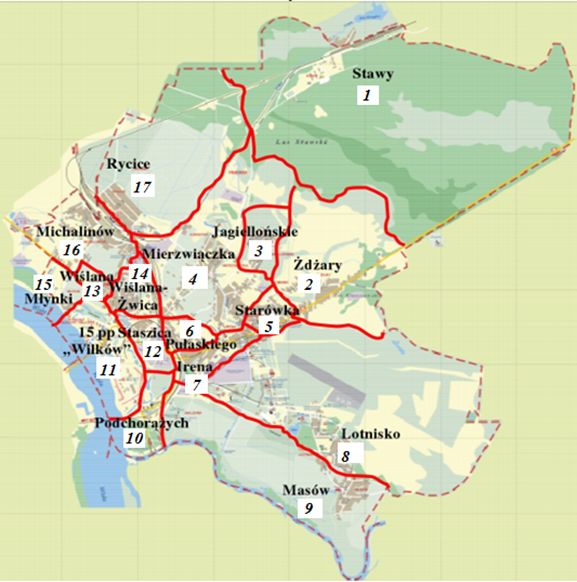
484 | Ł. Wojciechowski et al.

vantage of an electric utility vehicle is the lack of noise [21].     This work addresses the possibility of optimizing the
Garbage collection usually takes place in the early morning. route on which the city’s cleaning vehicle is moving to col-
Quiet electric drives do not disturb the residents. Another lect urban waste. Its aim is to present the conditions which
advantage of electric drives is the favourable torque param- influence the waste collection process in Dęblin and the
eters of the electric motor. What is more, there are usually possibility of its improvement.
no clutch or gearbox in the vehicles, which positively trans-         The conducted research, unlike the currently used
lates into the comfort of the driver. Electric vehicles are methods of delivery and planning, differs in the complexity
unfortunately much more expensive than their combustion of combining many methods into one hybrid computational
engine counterparts. However, the operating costs of elec- process. At the moment, popular algorithms used focus
tric vehicles are much lower. Especially when the energy for only on the separate optimization of one parameter, e.g.
charging electric vehicle batteries comes from renewable transport time, or the amount of raw material delivered, etc.
energy sources [13].                                              tasks in the working time of drivers. The presented method
     Another power unit used in city vehicles is the hybrid combines all aspects of collecting waste in terms of the se-
system. It usually consists of an internal combustion engine lection of vehicles, their working time, optimal routes and
and an electric motor [23]. The internal combustion engine including these tasks in the drivers’ working time.
is usually used for driving at higher speeds and with greater         The method is based on multi-criteria optimization for
loads. The electric motor is responsible for driving at low the collection and disposal of municipal waste by a spec-
speeds. It is also able to support the combustion engine ified number of means of transport. Currently, individual
during starting and acceleration. Dynamic phases in the transporting units have their own work plan. This results
operation of an internal combustion engine are usually in many delays, lack of adequate capacity or lack of syn-
responsible for high emissions of pollutants in the form of chronization of designated transport tasks with the given
nitrogen oxides in gasoline engines and particulate matter plan. Another hindering factor in the performance of the in-
in diesel engines. A very important advantage of hybrid tended task is the transport of waste to the collection point.
vehicles is the recovery of the braking energy by means As a result, there are limits to control over the vehicles that
of the electric motor. As a result, the range of the hybrid have completed their task and are ready for further oper-
vehicle can be increased by more than 10%.                        ation and the vehicles during the transport task. Verified
     Hydrogen vehicles have also been developing rapidly were the approximate times of shortening the operation of
in recent years [16]. These are vehicles powered by electric collecting municipal waste using the conventional method
motors. They are supplied with current from the hydrogen and with the use of the described algorithm. It was found
stored on board and compressed usually to 350 or 700 bar. that depending on the route, its length and the weight of
Hydrogen fuel cells are responsible for converting the chem- the transported waste, it is possible to gain a dozen or so
ical energy of hydrogen into electricity. The advantage of percent advantage during the performance of a given task.
hydrogen vehicles over electric vehicles with lithium-ion It is a modified and improved method of collecting munici-
batteries is a very short hydrogen refuelling time and a pal waste. The algorithm has control over all transport tasks
much greater range.                                               of vehicles and is able to optimally distribute tasks. This
     Another factor affecting the operating costs of a munic- eliminates longer journeys, transport downtime or over-
ipal cleaning company is the choice of an optimal route [24, lapping routes involving the same location. This results in
25]. The choice of the route and the resulting travel costs greater efficiency of the means of transport used, reduction
depend on the urban development pattern [26, 27]. Choos- of the time needed to perform a given operation and, con-
ing a vehicle with low consumption of inexpensive fuel and sequently, increased collection of municipal waste along
an optimal route for the transport task of collecting mu- with its delivery to the collection point.
nicipal waste may result in the lowest possible operating
costs of the vehicle fleet [28]. When optimizing the route,
algorithms for selecting the appropriate path are of great im-
portance [29, 30]. The present paper addresses the problem
                                                                  2 The problem of route mapping in
of optimizing the route along which a city cleaning vehicle           transport networks
travels in order to collect municipal waste [31]. Its purpose
is to present the conditions that affect the waste collection Considering the subject of optimization of transport activ-
process on the example of the city of Dęblin in Poland. The ity, it is impossible to ignore the problem of the travelling
paper also considers the possibilities of improving selected salesman, commonly referred to as the travelling salesman
transport processes in the collection of municipal waste.         problem (TSP). It is one of the combinatorial optimization
Route optimization for city cleaning vehicle | 485
problems, aimed at determining the shortest route between • to determine the nearest (adjacent) vertices for the
certain points, thus obtaining the lowest cost [32]. The task starting point, bearing in mind that the starting point
of the travelling salesman is to visit n cities (each exactly has the lowest cost of the route;
once) and return to the starting point (city). This means • indication of the next nearest neighbouring vertices,
that once all restrictions are taken into account, the route for selected neighbours, other than the once previ-
between A and B does not have to be the same as from B ously designated, together with a calculation of indi-
to A. The problem of salesman is related to the so called vidual costs generated for different combinations of
Hamiltonian cycle in the graph, which consists of a system the routes of the travelling salesman movement;
of vertices contained in it exactly once [31]. The route of the • the procedure is repeated in n steps, so that the ver-
salesman is created on the basis of n number of vertices, tices selected on the route of the travelling salesman
so that it is possible to return to the starting point using are different from each other.
the shortest possible route. This involves setting up such
The ‘nearest neighbour search’ method boils down to
a route that the lowest cost of its implementation will be
limiting the number of all route combinations so that sev-
achieved.
eral algorithms are created in each step. This task can also
The obtained result can be assigned, in terms of com-
be formulated using linear programming and the simplex
plexity, to an exponential class. This means that it’s neces-
method, with a target function:
sary to find the Hamilton cycle by calculating the sum of
n ∑︁ n
the edge weight and indicating its smallest value. In this ∑︁
K (x) = c ij x ij → min (1)
case, the required value is the distance between all points
i=1 j=1
under consideration.
In the case of the travelling salesman problem, the Where: x ij is a decision variable with values of one or zero,
length of the route is not always the main issue to be con- meaning the allocation of a given vertex to the optimal
sidered. The aim of the optimization can also be related to traveling salesman route.
the discovery of the shortest route in terms of travel time. With limitation:
In such a case ‘distance’ is considered as the duration of n
∑︁
the journey on individual sections. Another option may x ij = 1, (2)
be determined by cost. In considering such an option, the i=1
price of the journey between the points shall be taken as
the basic information. Finding a solution for all possible ∑︁n
variants would be very time-consuming, therefore the fol- x ij = 1, (3)
lowing methods are mainly used in order to solve the task j=1
of the travelling salesman, such as:
x ij = 1 or 0 (4)
• the ‘nearest neighbour search’ – consists in limiting
the number of all combinations for the route, reduc-
ing it to several variants at each step of the algorithm;
2.2 Ant colony optimization algorithm
• genetic algorithm – which is based on imitation of
natural processes occurring during evolution, such
By creating an ant colony optimization algorithm, the sci-
as genetic inheritance;
entists observed the social behaviour of an ant colony,
• ant colony optimization algorithm – a way of search-
in which survival depends on the degree of cooperation
ing solutions inspired by the behavior of Argentine
in achieving the goal i.e. looking for food or building on
ants looking for food in their colony.
anthill. Ants alone are not able to achieve the adopted mis-
sion, only in a group, which is based on the interaction
between all units of a given colony; their intelligence can
2.1 Nearest neighbour search method be seen. Ants have an instinct that does not fail them even
if they try to make their work more difficult by encoun-
The method includes limiting the number of all combina-
tering an obstacle on the road. Initially, their response is
tions for the route, reducing it to several variants at each
characterized by chaotic movements, but after a while they
step of algorithm. It is a process of searching for the optimal
manage to work out again the shortest way. This is done by
route of the travelling salesman that is a cycle with minimal
means of pheromones (infochemical compounds), which
cost. It consists of the following steps:
they leave in the environment. The whole decision-making486 | Ł. Wojciechowski et al.
process is presented in Figures 1–4. During the hike ants fol- by adding their own. The scent on the road is so high that
low the food and set out random routes. When any of them the whole colony starts to follow it (Figure 4). Over time, the
finds food, they leave the pheromone all the way back to pheromones lose their intensity as a result of evaporation,
the anthill. This is to set a path for other individuals which which leads to the disappearance of the pathway when the
is using their ability to sense there pheromones, follow the food runs out.
path by imitating the largest number of companions and
also leave a suitable trail (Figure 1).
Figure 4: The final path for the ant colony to get food
Figure 1: A diagram showing ants’ behaviour when searching for
food
An attempt to create an optimization algorithm based
on the behaviour of ant colonies has led to the develop-
If there is an obstacle, the ants must decide which road ment of the technique ‘Ant Colony Optimization’. This al-
to take, whether to turn right or left. The possibility of choos- gorithm is based on the principle that artificially created
ing any path is the same (Figure 2) ants’ colony work closely together to find the best solution
to difficult optimization problems. The key element is coop-
eration, because everyone can find a solution individually,
but only by taking joint actions can an optimal concept be
created.
In order to create an ant colony optimization algorithm
it is necessary to define components such as:
• Agencies – ‘ants’;
• Surroundings with specific paths of different lengths;
Figure 2: The ants’ behavioral pattern in case of an obstacle • ‘pheromones’ commanding movement of agents.
The principle of the form algorithm’s operation in the
context of the travelling salesman problems has been pre-
Individuals who choose a shorter route strengthen the
sented in a block diagram (Figure 5). It is based on a num-
pheromone trace, which settles on it faster than on the
ber of assumptions, established during the planning phase,
longer route, as on the shorter route less substance will
and the need to make decisions e.g.:
evaporate as opposed to the second choice (Figure 3).
• Each ant leaves a scented mark between the points of
the route, in a size equal to the inverse of the route;
• The first routes to be travelled are selected at random,
while the next ones are determined on the basis of
the resultant probability, which is a function of the
pheromone left and the distance between points;
• Individual points can only be visited once;
• The pheromone left by ants evaporates over time,
Figure 3: Diagram of path selection by ants after an obstacle has which should be taken into account at the planning
appeared on the road (creation) stage of the algorithm, using the coefficient
of evaporation; this avoids the accumulation of the
pheromone on the ‘worse’ routes and exposes the
The result is that all ants choose the shortest route, as
most commonly used routes.
they head towards the food by the use of the scent, more-
over they increase the intensity of the existing pheromoneRoute optimization for city cleaning vehicle | 487
better or worse. Those organisms that do better in the wild
have a better chance of surviving.
The relationship can be depicted from the relation be-
tween the mouse and the cat hunting it. A fast, agile and
clever cat is more likely to catch a mouse than a slow and
clumsy one. Therefore, this first cat will survive and will be
able to pass on its ‘better’ genes to future generations. Some
cats from the ‘worse sort’ will also survive, thus introduc-
ing a mixture of genetic material. The natural reaction of
the population is to strive for improvement (the ‘better’ or-
ganisms reproduce and the ‘worse’ organisms die out). The
genetic algorithm works on the basis of relations presented
in the Figure 6.
Figure 6: Genetic algorithm test area
Colorful circles (located in the middle of the test area)
depict individuals with specific information. In relation to
the problem of the travelling salesman, the wheels are cities,
while the information is a reference to their location on the
map, including the distance between them. The starting
point of the route planning is the black point, while the red
ones are the neighboring villages with the shortest distance
from the start. According to the genetic algorithm, they are
Figure 5: Diagram of operation based on form algorithm “better” than others. Therefore, in the first stage of route
planning, it is these cities that are taken into account, while
the others are initially rejected.
Only selecting the appropriate coefficients it is possible The selection of the initial population is made on the
to find the best solution to the problem, which will be opti- basis of the indication of the cities that need to be visited
mal for the assumptions made. At first, the ants move ran- by the travelling salesman. The first route is indicated at
domly, but after some time they are attracted to the ‘better’ random, eliminating from the list the cities already visited
paths, giving up those that do not meet their requirements. so as not to arrive twice. The assessment shall be based on
a comparison of the distance between the points concerned.
The best matching elements form the shortest route.
2.3 Genetic Algorithm The process is completed when:
• the optimal value was found (the shortest route was
The genetic algorithm was created on the basis of obser-
found, or the value was reached);
vations of nature and changes taking place in it. Optimal
• performing subsequent attempts does not allow to
solutions are searched by imitation of natural processes
find a better solution;
related to evolution, i.e. genetic inheritance. Every living or-
• some specified time passed or the indicated number
ganism lives in a changing environment to which it adopts
of attempts was over.488 | Ł. Wojciechowski et al.
In the genetic algorithm, points are selected to create a possible to distinguish between several types of mutations,
new route. i.e.:
• inversion – refers to indicating a fragment of the route
and then reversing the order of visited cities;
• insertion – consists in selecting a random city and
inserting it in any other place;
• relocation – is characterized by indicating a fragment
of the route and moving it to another place;
• mutual exchange – consists in selecting two cities
and swapping them with each other.
The process, which is unambiguous to the end of the
genetic algorithm, is stopped when the conditions are met.
The method of genetic algorithm for finding the optimal so-
lution for the travelling salesman problem does not always
bring about finding the optimal route, but always leads to
the best possible solution.
The subject matter of a single travelling salesman is an
exceptional problem in the field of vehicle route planning,
which is seen as a problem of many travelling salesmen.
When planning a route for many vehicles, it should be re-
membered to meet criteria such as:
• visiting individual customers by only one vehicle;
• the load capacity for each vehicle indicated for oper-
ation cannot be exceeded;
• the price (or length) of the routes covered by all vehi-
cles used must be the smallest.
Following these guidelines, two key issues arise in
route planning, i.e.:
Figure 7: A diagram showing the operation of a genetic algorithm • dividing the set of all points to be visited into regions,
where each area will be assigned to one vehicle;
• determining the order of visits of individual points
Two types of selection can be distinguished: within a given region.
• elite – is based on a better/worst order of values, from The problem of routes planning for vehicles is a start-
best to worst, the number of the best ones should be ing point on the basis of which it is possible to formulate
determined; derivative issues based on the modification of the basic
• tournament – is characterized by pairing and then task.
indicating the better solution in them.
Approaching the end of the process, two exemplary
routes intersect in order to create a new (better) road. This is 3 Waste management in Dęblin
done by using one of the three ways of crossing appropriate
for the travelling salesman problem: Each product (e.g. a raw material, material or final prod-
• with partial mapping (PMX); uct) which is not used in accordance with its performance
• with ordering (OX); characteristics becomes waste.
• cyclic (CX). The currently efficient waste management within a
given city or commune should be supported by modern
The last step in the genetic algorithm is to make a mu-
logistic solutions, i.e. the so called reverse logistics which
tation. It consists of exchanging one or more elements in
includes: waste logistics, reverse logistics, reprocessing, as
a given population. This is to introduce its variability. It is
well as recycling x. The aim of waste management logisticsRoute optimization for city cleaning vehicle | 489
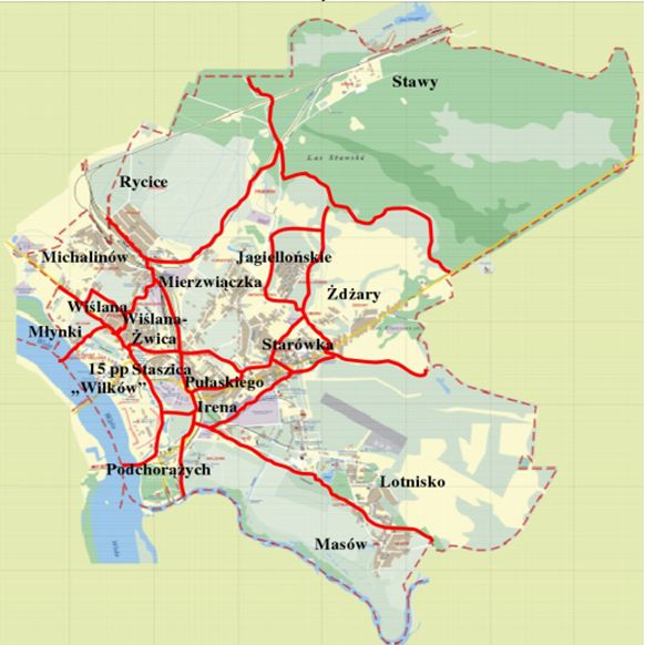
is to find the best solutions in terms of organization and • mixed development – i.e. agricultural-horticultural
cost for transport, storage, reprocessing and disposal of the and single-family, located along the main streets of
so-called rubbish. the city – dominates within the Irena, Michalinów,
Waste management in the area of a city or commune Mierzwiączka, Rycice, and Starówka estates.
comes down primarily to the collection of mixed and seg-
The principles of urban waste management in the area
regated urban waste by specialized waste disposal compa-
of the city of Dęblin have been developed in the document
nies.
entitled “Waste Management Plan for the town of Dęblin”.
In the area of Dęblin commune, 17 districts can be indi-
cated, which designate individual settlements, i.e.: Irena,
Jagiellońska, Lotnisko, Masów, Michalinów, Mierzwiączka,
Młynki, Podchorążych, Pułaskiego, 15 pp "Wików", Rycice,
Starowka, Staszica, Stawy, Wiślana, Wiślana-Żwica, Żdżary
(Figure 8).
Figure 9: Graphical route separation for a city cleaning vehicle [33]
According to this document, the collection and trans-
port of waste in Dęblin commune is the responsibility of
Miejski Zakład Gospodarki Komunalnej (MZGK) Sp. z o. o.
Figure 8: Administrative division of Dęblin [33] and auxiliary company Tonsmeier Wschód Sp. z o. o. from
Radom. Currently, waste collection is carried out from 13,711
inhabitants of the city and is selective for 99% of them. The
The division into individual districts is also determined
total amount of mixed and selective waste in 2019 was 4
by the type of housing development, which main investors
933 tones. Waste collection is carried out on the basis of a
were: the army, railways, the city, housing cooperatives and
specific schedule, which divides the city into three groups
individual investors. On this basis, the following housing
in the case of mixed waste collection and two groups in
estates and development complexes can be distinguished:
the case of segregated waste. The main problem of urban
• single-family development – dominates mainly in waste management in this city is the vast area and the lack
the following estates: Jagiellońska, Masów, Młynki, of landfill for mixed waste.
Pułaskiego, Wiślana-Żwica, and Żdżary; The process that requires improvement is the collection
• multi-family development – i.e. blocks of flats located of three different waste items, separated and mixed from
in the area of the Staszica, Stawy, Wiślana, Lotnisko, more than 816 points, which are distributed throughout the
and Podchorążych housing estates; city at different densities.
• low-intensity development – single-family houses When planning to optimize the work process for a city
with accompanying services located in the city centre cleaning vehicle, the daily time limit, i.e. the driver’s work-
are predominant; ing time, should be reduced to 8 hours. Additionally, in490 | Ł. Wojciechowski et al.
Table 1: Waste collection points on individual routes mance of the existing system and to plan a more beneficial
solution.
Route Approximate number of containers For the purpose of the submitted work, the problem has
number Single-family Multi-family Total been simplified by graphically separating the locations into
houses houses shorter routes covering the area of individual settlements.
1 - 3 3 The MZGK’s work system consists of providing employees
2 78 - 78 with a list of locations with a random order of points to be
3 89 - 89 served on a daily basis. The driver’s task is to serve everyone
4 138 2 140 within the set working time.
5 76 - 76
6 69 - 69
7 13 - 13
8 48 6 54 4 Optimization of the urban waste
9 75 - 75 collection route in Dęblin
10 7 4 11
11 - 12 12 The criteria for the optimization of work for the urban waste
12 9 6 15 treatment vehicle is the option of minimizing the length of
13 5 7 12 the route that the vehicle has to travel from the place of daily
14 47 - 47 stopover through specific collection points to the place of
15 32 - 32 cargo return, during the days of the week imposed by the
16 39 - 39 schedule. The basic constraints for route planning include
17 51 - 51 the capacity of the means of transport, the driver’s working
SUM 776 40 816 time and the location of the final destination. On the basis
of the presented data and collected information, the route
optimization model presented in Table 2 was developed.
the case of segregated waste, there is a limitation in the The main restrictive conditions in the form of state-
form of receiving only one type of raw material in a given ments Σ x = 1 and Σ x = 1 guarantee that the vehi-
jϵY ij iϵY ij
course. The collection of mixed waste generates additional cle will not miss any point that needs to be visited to collect
time losses when the car is full, because the waste collec- waste. The form s + t − (︀1 − x )︀ M < s qualifies a con-
i ij ij ij j
tion point (the so-called waste dump) is 20 km away from tinuity of the route that must be consistent between the
Dęblin. Here the contents of the garbage truck are unloaded individual points, i.e. when a vehicle collects waste from
and returned to the route for further collection. the first point it is followed by the second point, between
The collection of waste for disposal should take place which the difference cannot be less than the travel time
only when the bins are full. The problem is not only to between these points. Condition K ≤ s ≤ L specifies the
i i i
determine the optimal routes for vehicles collecting urban time slot within which the point should be visited.
waste, but also to indicate the location for the collection Thanks to such assumptions, it is possible to deter-
containers. According to the current policy in the company, mine the optimal time for a given day’s route. On the basis
routes are planned in an intuitive way based on the many of these assumptions, the person supervising the cleaning
years of experience of the employees, which prevents the works (in this case, urban waste collection) may verify the
use of available resources and possibilities in an optimal correctness of the route and, in case of an inappropriate
way. variant, develop a more beneficial variant. However, this
The shortcomings that occur in waste collection mainly decision model can only be used for a certain number of
concern the failure to meet accepted collection deadlines reception points and will not apply to a very large agglomer-
and the lack of predictability and transparency of the route. ation. Therefore, in order to use it, Dęblin was divided into
This leads to contradiction with the agreed waste collection individual housing estates, where the number of reception
schedule and errors are recorded in working system. In or- points was estimated, which is closely related to the type
der to be able to repair the system it is necessary to develop of development in a given housing estate.
a template with the locations of the individual waste bins Two different routes have been analyzed using the
and to determine the estimated distances between them. above decision-making model: one housing estate with
On this basis it would be possible to determine the perfor- single-family houses and the other with multi-family
houses. The whole process of research was carried out inRoute optimization for city cleaning vehicle | 491
Table 2: Routing optimization model for the urban cleaning vehicle in Dęblin
Data in the content of the work and parameters from Table 5
Y – set of all nodes
Z – specific set of connections
Parameters c i,j – length of the connection i, j
t i,j – travel time
K i – start of time for point i
L i – end of time for point i
X(i, j) assuming a value of 1, when edge i, remains within the range of solutions
Decision variables
Si which is the time of arrival at point i
Goals’ function min Σ (i,j)ϵA c ij x ij
Σ jϵY x ij = 1 when i ∈ Y
Σ iϵY x ij = 1 when j ∈ Y
(︀ )︀
s i + t ij − 1 − x ij M ij < s j when (i, j ≠= 1) ∈ Z
Restrictive conditions
K i ≤ s i ≤ L i when j ∈ Y
x i,j ϵ{0, 1} when (i, j) ∈ Z
s i ≥ 0 when i ∈ V
several steps. The first step involved calculation for the
route that was being driven on a daily basis by an employee
of MZGK within the indicated housing estate. In this case it
is difficult to estimate a fixed route and a clear action plan,
as this option provides an alphabetical list of the locations
that have to be visited by the indicated crew.
In the second stage, the completed route, which was
registered by the GPS transmitter during the measurements
performed on 25 July 2019, was transferred to the estate plan.
The result of this step is the presentation of the individual
points of stopping the car as a result of successive trans-
mitter readings. The calculation of distance and travel time
was estimated on the basis of average travel times read from
the recorder connected to the GoogleMaps application.
The third step of the research included an attempt to
optimize the route on the basis of the decision model pre-
sented in Table 2. The tests were based on the average speed
of a moving vehicle (9 km/h approximately 2.5 m/s) and a
stop (45 s for mixed waste and 20 s for segregated waste, re-
spectively), which took place during the collection of waste
from one container located at particular points.
The basic optimization criterion was the length of the
Source: www.google.pl/maps
route. Route 3, which includes the Jagiellonian housing
estate, was chosen for the study. The tests were carried Figure 10: Visualization of the Jagiellońska housing estate (route no.
out in two working days to make measurements for the 3) including the initial and final waste collection points on a straight
collection of mixed and segregated waste. road section
In the case of route number 3, the city cleaning team
had waste from 89 locations to collect. The estate consists In the first case, the measurements were taken for the
of 15 streets. To facilitate the calculation and legibility of collection of mixed waste, assuming the speed of move-
the diagram, the initial and final point of the street or near ment of 9 km/h and the time of stopping for emptying the
an intersection is taken into account, as shown in Figure 10. container of 45 s. The route the team was moving according492 | Ł. Wojciechowski et al.
Table 3: List of the route followed by MZGK employees during the collection of mixed waste
Route section Length of the Travel time Number of pick-up Stopover time at Total time
no. 3 section [km] [min] points points [min] [min]
1-2 0.5 3.3 1 0.75 4.05
2-28 1.3 8.6 3 2.25 10.85
28-25 0.7 4.6 2 1.5 6.1
25-23 0.3 2 0 0 2
23-24 0.4 2.6 1 0.75 3.35
24-17 1.2 8 5 3.75 11.75
17-18 0.5 3.3 0 0 3.3
18-22 0.9 6 4 3 9
22-20 0.6 4 2 1.5 5.5
20-21 0.4 2.6 2 1.5 4.1
21-20 0.4 2.6 2 1.5 4.1
20-18 0.3 2.6 1 0.75 3.35
18-19 0.4 2.6 2 1.5 4.1
19-16 1.5 10 4 3 13
16-4 1.3 8.6 4 3 11.6
4-5 0.4 2.6 0 0 2.6
5-14 0.9 6 3 2.25 8.25
14-15 1.1 7.3 4 3 10.3
15-14 1.1 7.3 3 2.25 9.55
14-5 0.9 6 4 3 9
5-6 0.6 4 0 0 4
6-12 1.4 9.3 4 3 12.3
12-13 1.1 7.3 3 2.25 9.55
13-12 1.1 7.3 4 3 10.3
12-8 1.4 9.3 2 1.5 10.8
8-9 0.4 2.6 1 0.75 3.35
9-10 0.8 5.3 2 1.5 6.8
10-11 0.9 6 3 2.25 8.25
11-10 0.9 6 3 2.25 8.25
10-9 0.8 5.3 4 3 8.3
9-8 0.4 2.6 0 0 2.6
8-6 0.6 4 0 0 4
6-7 0.4 2.6 1 0.75 3.35
7-4 1.7 11.3 0 0 11.3
4-26 0.7 4.6 0 0 4.6
26-27 0.9 6 3 2.25 8.25
27-29 1.0 6.6 3 2.25 8.85
29-30 0.4 2.6 0 0 2.6
30-31 1.1 7.3 3 2.25 9.55
31-32 1.0 6.6 2 1.5 8.1
32-4 0.3 2.6 0 0 2.6
4-3 0.9 6 2 1.5 7.5
3-2 1.2 8 2 1.5 9.5
Total 35.1 233.8 89 66.75 300.55Route optimization for city cleaning vehicle | 493
Table 4: Summary of the route of mixed waste collection after optimization by means of a decision model
Route section Length of the Travel time Number of pick-up Stopover time at Total time
no. 3 section [km] [min] points points [min] [min]
1-7 4.3 28.6 6 4.5 33.1
7-6 0.4 2.6 0 0 2.6
6-8 0.6 4 0 0 4
8-9 0.4 2.6 1 0.75 3.35
9-10 0.8 5.3 6 4.5 9.8
10-11 0.9 6 3 2.25 8.25
11-10 0.9 6 3 2.25 8.25
10-12 0.4 2.6 0 0 2.6
12-13 1.1 7.3 3 2.25 9.55
13-12 1.1 7.3 4 3 10.3
12-6 1.4 9.3 6 4.5 13.8
6-5 0.6 4 0 0 4
5-14 0.9 6 7 5.25 11.25
14-15 1.1 7.3 4 3 10.3
15-14 1.1 7.3 4 3 10.3
14-16 0.4 2.6 0 0 2.6
16-19 1.5 10 4 3 13
19-18 0.4 2.6 2 1.5 4.1
18-20 0.3 2.6 1 0.75 3.35
20-21 0.4 2.6 2 1.5 4.1
21-20 0.4 2.6 2 1.5 4.1
20-22 0.6 4 2 1.5 5.5
22-18 0.9 6 4 3 9
18-17 0.5 3.3 0 0 3.3
17-23 0.8 5.3 4 3 8.3
23-24 0.4 2.6 1 0.75 3.35
24-23 0.4 2.6 0 0 2.6
23-25 0.3 2.6 0 0 2.6
25-28 0.7 4.6 2 1.5 6.1
28-29 0.4 2.6 2 1.5 3.35
29-26 1.9 12.6 6 4.5 17.1
26-32 0.4 2.6 4 3 5.6
32-30 2.1 14 5 3.75 17.75
30-2 0.3 2.6 1 0.75 3.35
2-1 0.5 3.3 0 0 3.3
Total 29.6 197.9 89 66.75 263.9
Table 5: Comparison of the length of the routes and their travel time for the compiled variants
Options under consideration for the survey Route length Time travel with waste collection
The route followed by MZGK employees 35.1 km 300.55 min
Optimized route 29.6 km 263.9 min494 | Ł. Wojciechowski et al.
Table 6: List of the route followed by MZGK employees during the collection of segregated waste
Route section Length of the Travel time Number of pick-up Stopover time at Total time
no. 3 section [km] [min] points points [min] [min]
1-2 0.5 3.3 1 0.3 3.6
2-28 1.3 8.6 3 0.9 9.5
28-25 0.7 4.6 2 0.6 5.2
25-23 0.3 2 0 0 2
23-24 0.4 2.6 1 0.3 2.9
24-17 1.2 8 5 1.5 9.5
17-18 0.5 3.3 0 0 3.3
18-22 0.9 6 4 1.2 7.2
22-20 0.6 4 2 0.6 4.6
20-21 0.4 2.6 2 0.6 3.2
21-20 0.4 2.6 2 0.6 3.2
20-18 0.3 2.6 1 0.2 2.8
18-19 0.4 2.6 2 0.6 3.2
19-16 1.5 10 4 1.2 11.2
16-4 1.3 8.6 4 1.2 9.8
4-5 0.4 2.6 0 0 2.6
5-14 0.9 6 3 0.9 6.9
14-15 1.1 7.3 4 1.2 8.5
15-14 1.1 7.3 3 0.9 8.2
14-5 0.9 6 4 1.2 7.2
5-6 0.6 4 0 0 4
6-12 1.4 9.3 4 1.2 10.5
12-13 1.1 7.3 3 0.9 8.2
13-12 1.1 7.3 4 1.2 8.5
12-8 1.4 9.3 2 0.6 9.9
8-9 0.4 2.6 1 0.3 2.9
9-10 0.8 5.3 2 0.6 5.9
10-11 0.9 6 3 0.9 6.9
11-10 0.9 6 3 0.9 6.9
10-9 0.8 5.3 4 1.2 6.5
9-8 0.4 2.6 0 0 2.6
8-6 0.6 4 0 0 4
6-7 0.4 2.6 1 0.3 2.9
7-4 1.7 11.3 0 0 11.3
4-26 0.7 4.6 0 0 4.6
26-27 0.9 6 3 0.9 6.9
27-29 1.0 6.6 3 0.9 7.5
29-30 0.4 2.6 0 0 2.6
30-31 1.1 7.3 3 0.9 8.2
31-32 1.0 6.6 2 0.6 7.2
32-4 0.3 2.6 0 0 2.6
4-3 0.9 6 2 0.6 6.6
3-2 1.2 8 2 0.6 8.6
Total 35.1 233.8 89 26.6 260.4Route optimization for city cleaning vehicle | 495
Table 7: Statement of the route of the waste collection after optimization by means of a decision model
Route section Length of the Travel time Number of pick-up Stopover time at Total time
no. 3 section [km] [min] points points [min] [min]
1-7 4.3 28.6 6 1.8 30.4
7-6 0.4 2.6 0 0 2.6
6-8 0.6 4 0 0 4
8-9 0.4 2.6 1 0.3 2.9
9-10 0.8 5.3 6 1.8 7.8
10-11 0.9 6 3 0.9 6.9
11-10 0.9 6 3 0.9 6.9
10-12 0.4 2.6 0 0 2.6
12-13 1.1 7.3 3 0.9 8.2
13-12 1.1 7.3 4 1.2 8.5
12-6 1.4 9.3 6 1.8 11.1
6-5 0.6 4 0 0 4
5-14 0.9 6 7 2.1 8.1
14-15 1.1 7.3 4 1.2 8.5
15-14 1.1 7.3 4 1.2 8.5
14-16 0.4 2.6 0 0 2.6
16-19 1.5 10 4 1.2 11.2
19-18 0.4 2.6 2 0.6 3.2
18-20 0.3 2.6 1 0.3 2.9
20-21 0.4 2.6 2 0.6 3.2
21-20 0.4 2.6 2 0.6 3.2
20-22 0.6 4 2 0.6 4.6
22-18 0.9 6 4 1.2 7.2
18-17 0.5 3.3 0 0 3.3
17-23 0.8 5.3 4 1.2 6.5
23-24 0.4 2.6 1 0.3 2.9
24-23 0.4 2.6 0 0 2.6
23-25 0.3 2.6 0 0 2.6
25-28 0.7 4.6 2 0.6 5.2
28-29 0.4 2.6 2 0.6 3.2
29-26 1.9 12.6 6 1.8 14.4
26-32 0.4 2.6 4 1.2 3.8
32-30 2.1 14 5 1.5 15.5
30-2 0.3 2.6 1 0.3 2.9
2-1 0.5 3.3 0 0 3.3
Total 29.6 197.9 89 26.6 224.5
Table 8: Comparison of the length of the routes and their travel time for the compared variants
Options under consideration for the survey Route length Time travel with waste collection
The route followed by MZGK employees 35.1 km 260.4 min
Optimized route 29.6 km 224.5 min496 | Ł. Wojciechowski et al.
to their own intuition is presented in Table 3, taking into The service of all pick-up points is unchanged as the
account the length of the section and the time needed to number of containers to be emptied remains the same.
cover it. The final travel time for collecting segregated waste from
The table below shows that the route followed by MZGK all points has decreased to about 3 hours, excluding un-
employees based on GPS records is 35.1 km. The journey planned stops.
of this section at a speed of 9 km/h without stopping for The time difference between the route taken by MZGK
waste collection takes about 4 hours on average. Taking into employees and the optimized variant is about 35 minutes
account all the houses that are located on this estate and (Table 8). This time is sufficient to speed up the process of
assuming that each property has only one container this collecting the next raw material after emptying the trailer.
time is extended by about 1 hour 7 min. The measurements In the case of segregated materials, the time of delivery
show that the average time spent by the employees on the to the collection point is much shorter due to its location
task of collecting municipal waste for this housing estate within the city.
is about 5 hours. The analysis shows that the use of even the simplest
After applying optimization mechanisms, the length route optimization methods for an urban waste cleaning
of the route decreased to 29.6 km, and the expected time vehicle contributes to shortening the driver’s working time
of driving along the designated route was about 3 hours and speeding up collection in individual regions. As a result
and 17 minutes. The service time of all the containers is of the research carried out, it was found that the freedom
constant, as the quantity remains the same. The final time left to drivers adversely affects the implementation of the
of waste collection from all points decreased to about 4h whole process and generates deviations from the actual
excluding unplanned stops (Table 4). time needed to make a given journey. Leaving the route
The difference between the route adopted by employ- arrangement to the driver’s freedom generates very long
ees and the mathematically optimized option is a total of 5.5 delays for the entire waste collection schedule, resulting in
km. The time difference is about 37 minutes of work. This overtime. Managers should analyze all the possibilities of
is the time that can be used to get to the waste collection a given route and analyze the acceptance schedule in order
point or in the case of loading capacity, a quicker route on to work out the most advantageous solutions.
the next housing estate (Table 5).
In the second case, the measurements were made for
the collection of segregated waste, assuming a speed of 9
km/h and a stopover time for emptying the container of
5 Conclusion
20 s. An additional limitation was the possibility of col-
The presented route optimization solution for a vehicle col-
lecting only one type of waste during one course. Due to
lecting urban waste (both mixed and segregated) is a simple
the schematic course, the measurements were made only
method of determining the order of driving through individ-
during plastic waste collection. The route the crew was
ual city streets. The prepared solution is universal and is
travelling according to their own intuition is presented in
not limited only to the surveyed housing estate. It presents
Table 6, taking into account the length of the section and
a pattern that can be applied to other routes in a similar
the time needed to complete it.
way. Shortening the distance and thus the working time is a
Table 6 below shows that MZGK employees operate
result of minimizing empty runs and moving several times
in a schematic manner and follow the same route as dur-
over the same section.
ing the collection of segregated materials. The route is 35.1
Implementation of the presented algorithm and its re-
km long. The journey of this section at a speed of 9 km/h
sults clearly indicate the reduction of the time of waste
without stopping takes about 4 hours on average. Taking
collection and delivery to the collection point and the ap-
into account all the pick-up points which are located on
propriate selection of available means of transport. This has
this housing estate and assuming that each property has
resulted in a reduction of idle downtime and an increase in
only one container, the travel time is extended by about
the efficiency of the entire waste disposal process, which
26 minutes. The measurements show that the average time
would take more time and effort in the case of conventional
the employees spend on the task of collecting segregated
methods.
waste for this housing estate is about 4.5 hours.
The proposed methodology in terms of practical appli-
After applying the optimization mechanisms presented
cations directly affects the synchronization of waste trans-
in the first variant of the study, it was possible to shorten
port in terms of the load capacity of transport means. This
the route to 29.6 km, while the expected time of travel was
translates into the optimal distribution of the waste load of
reduced to about 3 hours and 17 minutes (Table 7).Route optimization for city cleaning vehicle | 497
vehicles ready for the performance of transport tasks. This [9] Skrucany T, Kendra M, Stopka O, Milojević S, Figlus T, Csiszar
results in a lack of delays and eliminates the reporting of C. Impact of the electric mobility implementation on the Green-
house Gases production in Central European Countries. Sustain-
more vehicles for the transport task than necessary.
ability. 2019;11:1-15.
The proposed solution also has limitations, resulting
[10] Correa G, Muñoz P, Falaguerra T, Rodriguez C.R. Performance
from the vast area and number of locations to be served. comparison of conventional, hybrid, hydrogen and electric urban
The company in the area of Dęblin has the task of collecting buses using well to wheel analysis. Energy. 2017;141:537-49.
waste from 819 points. Developing an optimal route for so [11] Pielecha I, Pielecha J. Simulation analysis of electric vehicles en-
many values requires very complicated calculations and ergy consumption in driving tests. Eksploatacja i Niezawodnosc
– Maintenance and Reliability. 2020;22 (1):130–137. DOI: http:
would not reflect the real possibilities of waste collection
//dx.doi.org/10.17531/ein.2020.1.15.
by employees and MZGK Company. The prepared solution [12] Barta D, Mruzek M, Kendra M, Kordos P, Krzywonos L. Using
can be used as an instruction to take the first steps to opti- of non-conventional fuels in hybrid vehicle drives. Advances in
mize the operation of the vehicle and as an initial point for Science and Technology Research Journal. 2016;10(32):240-47.
further modifications of the operating system. [13] Małek A, Caban J, Wojciechowski Ł. Charging electric cars as
a way to increase the use of energy produced from RES. Open
Future works will be aimed at improving the efficiency
Engineering. 2020;10(1):98-104, DOI:10.1515/eng-2020-0009.
of the system in terms of organization and scheduling of
[14] Elnajjar E, Hamdan MO, Selim MYE. Experimental investigation
transport tasks of the means of transport used for waste of dual engine performance using variable LPG composition
collection. The disadvantages may consist in discrepan- fuel. Renewable Energy. 2013;56:110-116, DOI: https://doi.org/
cies in the reported weight and dimensions of the material 10.1016/j.renene.2012.09.048.
intended for transport. [15] Synák F, Čulík K, Rievaj V, Gaňa J. Liquefied petroleum gas as an
alternative fuel. Transportation Research Procedia. 2019;40:527-
534, DOI: 10.1016/j.trpro.2019.07.076.
[16] Fragiacomo P, Piraino F, Genovese M. Insights for Industry
References 4.0 Applications into a Hydrogen Advanced Mobility. Proce-
dia Manufacturing. 2020;42:239-245. https://doi.org/10.1016/
j.promfg.2020.02.077.
[1] Buhrkal K, Larsen A, Ropke S. The Waste Collection Vehicle Rout-
[17] Datta A., Mandal B.: A comprehensive review of biodiesel as
ing Problem with Time Windows in a City Logistics Context. Pro-
an alternative fuel for compression ignition engine. Renew-
cedia - Social and Behavioral Sciences. 2012;39:241-254. DOI:
able and Sustainable Energy Reviews. 2016;57:799–821, DOI:
https://doi.org/10.1016/j.sbspro.2012.03.105.
10.1016/j.rser.2015.12.170.
[2] Bányai T, Tamás P, Illés B, Stankevi Z, Bányai A. Optimiza-
[18] Hunicz J, Matijošius J, Rimkus A, Kilikevičius A, Kordos P, Mikul-
tion of Municipal Waste Collection Routing: Impact of Indus-
ski M. Eflcient hydrotreated vegetable oil combustion under
try 4.0 Technologies on Environmental Awareness and Sus-
partially premixed conditions with heavy exhaust gas recircula-
tainability. Int. J. Environ. Res. Public Health. 2019;16:634.
tion. Fuel. 2020;268:117350, DOI: https://doi.org/10.1016/j.fuel.
DOI:10.3390/ijerph16040634.
2020.117350.
[3] He Z, Li Q, Fang J. The solutions and recommendations
[19] Lewicki W. The case study of the impact of the costs of operational
for logistics problems in the collection of medical waste in
repairs of cars on the development of electromobility in Poland.
China. Procedia Environmental Sciences. 2016;31:447–456. DOI:
The Archives of Automotive Engineering – Archiwum Motoryzacji.
10.1016/j.proenv.2016.02.099.
2017;4:107-16.
[4] Stopka O, Šarkan B, Vrabel J, Caban J. Investigation of fuel con-
[20] Šarkan B., Kuranc A., Kučera L.: Calculations of exhaust emis-
sumption of a passenger car depending on aerodynamic resis-
sions produced by vehicle with petrol engine in urban area. IOP
tance and related aspects: a case study. The Archives of Automo-
Conference Series: Materials Science and Engineering. 2019, 710,
tive Engineering – Archiwum Motoryzacji. 2018;3.
1, DOI: 10.1088/1757-899X/710/1/012023.
[5] Šarkan B, Skrúcaný T, Semanová Š, Madleňák R, Kuranc A, Se-
[21] Vepsäläinen J, Otto K, Lajunen A, Tammi K. Computationally efl-
jkorová M, Caban J. Vehicle coast-down method as a tool for
cient model for energy demand prediction of electric city bus in
calculating total resistance for the purposes of type-approval
varying operating conditions. Energy. 2019;169:433-43.
fuel consumption. Zeszyty Naukowe. Transport / Politechnika
[22] Jin X, Li J, Wu P, Zhang X. Researches on Modeling Methods of
Śląska. 2018;98.
Battery Capacity Decline Based on Cell Voltage Inconsistency
[6] Lebkowski A. Studies of Energy Consumption by a City Bus Pow-
and Probability Statistics. Energy Procedia. 2016;88:668–74.
ered by a Hybrid Energy Storage System in Variable Road Condi-
[23] Caban J, Zarajczyk J, Szmigielski M, Górniak B. Hybrid drive as
tions. Energies. 2019;12:951.
a future in agricultural technology. Zeszyty Naukowe Instytutu
[7] Šarkan B, Gnap J, Kiktová M. The importance of hybrid vehicles
Pojazdów / Politechnika Warszawska. 2018;3.
in urban traflc in terms of environmental impact. The Archives of
[24] Keil R, Krone D, Kremenova I, Madlenak R. Communications net-
Automotive Engineering – Archiwum Motoryzacji. 2019;85(3):115-
works as base for mobility – trend development of network archi-
22. DOI:10.14669/AM.VOL85.ART8
tectures. Communications – Scientific Letters of the University
[8] Caban J, Zarajczyk J, Małek A. Possibilities of using electric drives
of Zilina. 2015;2:80-85.
in city buses. Proceeding of 23rd International Scientific Confer-
[25] Szmelter-Jarosz A, Rześny-Cieplińska J. Priorities of Urban Trans-
ence Transport Means. 2019:543-547.
port System Stakeholders According to Crowd Logistics Solu-498 | Ł. Wojciechowski et al.
tions in City Areas. A Sustainability Perspective. Sustainability. [30] Matusiewicz M, Rolbiecki R, Foltyński M. The Tendency of Urban
2020;12;317. DOI:10.3390/su12010317 Stakeholders to Adopt Sustainable Logistics Measures on the
[26] Chocholac J, Sommerauerova D, Hyrslova J, Kucera T, Hruska R, Example of a Polish Metropolis. Sustainability. 2019;11:5909.
Machalik S. Service quality of the urban public transport compa- DOI:10.3390/su11215909.
nies and sustainable city logistics. Open Eng. 2020;10:86–97. [31] Droździel P., Winska M., Madlenak R., Szumski P.: Optimization
DOI: https://doi.org/10.1515/eng-2020-0010 of the post logistics network and location of the local distri-
[27] Sanchez-Diaz I, Palacios-Argüello L, Levandi A, Mardberg, bution center in selected area of the Lublin province. 12th In-
Basso J.R. A Time-Eflciency Study of Medium-Duty Trucks De- ternational Scientific Conference of Young Scientists on Sus-
livering in Urban Environments. Sustainability. 2020;12:425. tainable, Modern and Safe Transport. Edited by: Bujnak J.,
DOI:10.3390/su12010425 Guagliano M. Procedia Engineering. 2017, 192, 130–135. DOI:
[28] Kiba-Janiak M, Witkowski J. Sustainable Urban Mobility 10.1016/j.proeng.2017.06.023.
Plans: How Do They Work? Sustainability. 2019;11:4605. [32] Diederik P, Kingma J, Ba A. A Method for Stochastic Optimization.
DOI:10.3390/su11174605. 3rd International Conference on Learning Representations, 2015.
[29] de Oliveira LK, Vieira Bertoncini B, de Oliveira C, Nascimento L et [33] http://deblin.e-mapa.net/ [access 2020.07.09]
al. Factors Affecting the Choice of Urban Freight Vehicles: Issues
Related to Brazilian Companies. Sustainability. 2019;11:7010.
DOI:10.3390/su11247010You can also read