Satellite-observed monthly glacier and snow mass changes in southeast Tibet: implication for substantial meltwater contribution to the Brahmaputra
←
→
Page content transcription
If your browser does not render page correctly, please read the page content below
The Cryosphere, 14, 2267–2281, 2020
https://doi.org/10.5194/tc-14-2267-2020
© Author(s) 2020. This work is distributed under
the Creative Commons Attribution 4.0 License.

Satellite-observed monthly glacier and snow mass changes in
southeast Tibet: implication for substantial meltwater
contribution to the Brahmaputra
Shuang Yi1,2 , Chunqiao Song3 , Kosuke Heki2 , Shichang Kang4,5 , Qiuyu Wang6 , and Le Chang6
1 Institute
          of Geodesy, University of Stuttgart, 70174 Stuttgart, Germany
2 Department  of Earth and Planetary Sciences, Hokkaido University, Sapporo, 060-0808 Japan
3 Key Laboratory of Watershed Geographic Sciences, Nanjing Institute of Geography and Limnology,

Chinese Academy of Sciences, Nanjing, 210008, China
4 State Key Laboratory of Cryospheric Science, Northwest Institute of Eco-Environment and Resources,

Chinese Academy of Sciences, Lanzhou 730000, China
5 CAS Center for Excellence in Tibetan Plateau Earth Sciences, CAS, Beijing 100101, China
6 Key Laboratory of Computational Geodynamics, University of Chinese Academy of Sciences, Beijing 100049, China

Correspondence: Shuang Yi (shuangyi.geo@gmail.com)

Received: 7 September 2019 – Discussion started: 18 November 2019
Revised: 29 May 2020 – Accepted: 18 June 2020 – Published: 21 July 2020

Abstract. High-Asia glaciers have been observed to be re-         gent modelling estimates and underlines the importance of
treating the fastest in the southeastern Tibet Plateau (SETP),    meltwater to the Brahmaputra streamflow. The high sensi-
where vast numbers of glaciers and amounts of snow feed the       tivity between GS melting and temperature on both annual
streamflow of the Brahmaputra, a transboundary river linking      and monthly scales suggests that the Brahmaputra will suffer
the world’s two most populous countries, China and India.         from not only changes in total annual discharge but also an
However, the low temporal resolutions in previous observa-        earlier runoff peak due to ongoing global warming.
tions of glacier and snow (GS) mass balance obscured the
seasonal accumulation–ablation variations, and their mod-
elling estimates were divergent. Here we use monthly satel-
lite gravimetry observations from August 2002 to June 2017        1   Introduction
to estimate GS mass variation in the SETP. We find that the
“spring-accumulation-type” glaciers and snow in the SETP          The Tibetan Plateau, considered the Asian water tower, is the
reach their maximum in May. This is in stark contrast to          source of several major river systems. The upper streams of
seasonal variations in terrestrial water storage, which is con-   these rivers are fed by rainfall, base flow, and widespread
trolled by summer precipitation and reaches the maximum           glacier and snow (GS) melt (Barnett et al., 2005; Immerzeel
in August. These two seasonal variations are mutually or-         et al., 2010; Jansson et al., 2003; Lutz et al., 2014). The GS
thogonal and can be easily separated in time-variable grav-       melt is susceptible to climate change, while its sustainable
ity observations. Our GS mass balance results show a long-        supply is critical to the local freshwater security, flood pre-
term trend of −6.5±0.8 Gt yr−1 (or 0.67±0.08 m w.e. yr−1 )        vention and control, and hydroelectric development (Bolch
and annual mass decreases ranging from −49.3 to −78.3 Gt          et al., 2012; Kaser et al., 2010; Yao et al., 2012). The south-
with an average of −64.5 ± 8.9 Gt in the SETP between             eastern Tibetan Plateau (SETP), including the Nyenchen
August 2002 and June 2017. The contribution of summer             Tanglha Mountains (NTM) and eastern Himalayas, holds
meltwater to the Brahmaputra streamflow is estimated to be        10 439 glaciers with a total area of 9679 km2 (RGI Consor-
51 ± 9 Gt. This result could help to resolve previous diver-      tium, 2017) and widespread seasonal snow coverage of up
                                                                  to 100 000 km2 . These maritime glaciers are characterized

Published by Copernicus Publications on behalf of the European Geosciences Union.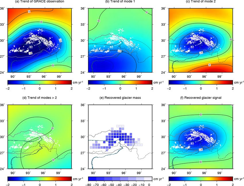
2268                                   S. Yi et al.: Implication for substantial meltwater contribution to the Brahmaputra

by low equilibrium-line altitudes with large topographic gra-     ments in spatial resolution in HMA glacier mass change stud-
dients (Yao et al., 2012) and the most severe mass loss in        ies, there has been little advance in their temporal resolution.
high-mountain Asia (HMA; Brun et al., 2017; Kääb et al.,             Observations at a monthly temporal resolution are nec-
2015). The GS melt serves as an essential water supplier for      essary to separately quantify summer and winter mass bal-
the Brahmaputra river system (e.g. Immerzeel et al., 2010;        ances, two processes dominating the annual glacier mass bal-
Lutz et al., 2014), which runs through three densely popu-        ance (Cogley et al., 2011, pp. 61–62) and thus crucial for the
lated countries, China, India and Bangladesh (Fig. 1). The        calibration and validation of glaciological models. The am-
revealed vulnerability of glaciers in the Brahmaputra basin       plitude of seasonal variation in the glaciers in the SETP is up
to global warming and emerging controversies over water al-       to ∼ 3 m w.e. (Wang et al., 2017), far exceeding their net an-
location (e.g. dam building; Tanck and Fazani, 2010) are in-      nual change of ∼ 0.6 m w.e. (Brun et al., 2017). Hence, the
creasingly attracting scientific and public concerns.             long-term trend of GS mass changes only reflects a small
   Due to the lack of observational data, most of the previ-      net imbalance of their ablation and accumulation. Monthly
ous estimates on the contribution of seasonal meltwater to        observations by GRACE since its launch in 2002 (Tapley et
the upstream flow of the Brahmaputra river were based on          al., 2004) are promising in identifying these two processes.
modelling approaches that were only calibrated by employ-         Up to now, the application of GRACE in HMA glaciers has
ing streamflow data. As a result, the previous estimates dis-     been focusing on their secular changes with little attention
agree widely from 19 % to 35 % (Table 1) due to different         to the seasonal variations (Gardner et al., 2013; Matsuo and
forcing data and approaches without direct constraints on GS      Heki, 2010; Yi and Sun, 2014). This is mostly due to the poor
mass balance (Bookhagen and Burbank, 2010; Chen et al.,           spatial resolution of GRACE (> 300 km) and the dominance
2017; Huss et al., 2017; Immerzeel et al., 2010; Lutz et al.,     of terrestrial hydrological signals in the seasonal gravity sig-
2014; Zhang et al., 2013). The amount of meltwater could          nals, which is difficult to eliminate from glacial signals. The
be even more divergent. For example, Huss et al. (2017) es-       latter limitation is particularly severe in the SETP with in-
timated that the amount of annual GS melt to the Brahma-          tense monsoon precipitation. The GS and hydrological mass
putra river was 138 km3 w.e. (water equivalent) yr−1 , which      changes (mainly including mass changes in rivers, soil mois-
is however triple the estimate of 43 km3 w.e. yr−1 by Lutz        ture and groundwater) dominate the seasonal gravity signals
et al. (2014). Although these two studies covered different       in the SETP observed by GRACE. Despite the general dif-
ranges, the glacierized zone in the basin was well enclosed in    ficulty in separating them in the spatial domain, we find it
both, so the estimates should not be so different. Such huge      possible to separate the two signals in the time domain, ow-
discrepancies in previous estimates make it imperative to in-     ing to their contrasting seasonal behaviours.
corporate the calibration from GS mass balance observations          Precipitation in the SETP is controlled by various atmo-
into future modelling experiments. Recently, the concept of       spheric circulation systems in different seasons, with west-
assimilating more GS observations has begun to be imple-          erly winds and the Bay of Bengal vortex in winter and spring
mented in state-of-the-art models (Wijngaard et al., 2017;        and the Indian monsoon in summer (Wu et al., 2011; Yang
Biemans et al., 2019), but their glacier results suffered from    et al., 2013; Yao et al., 2012). The first two systems were
coarse temporal resolution (two observations over 5 years)        found to drive the spring precipitation in the SETP along
and the snow mass changes were partially constrained by           the Brahmaputra river, thus forming a “spring-accumulation”
area changes.                                                     type of glacier (Yang et al., 2013). The Indian monsoon pre-
   Spaceborne sensors can be helpful in this desolate moun-       vails from June to September and brings intense precipitation
tain region. Remote sensing techniques for regionwide GS          to the southern side of the Himalayas, where terrestrial wa-
mass balance measurements can be divided into three cat-          ter storage shows tremendous seasonal changes and peaks
egories: laser altimetry (e.g. Ice, Cloud and land Elevation      in late summer. Therefore, according to the climate stations
Satellite – ICESat – Kääb et al., 2012), multi-temporal digital   near NTM, we can observe bimodal precipitation variations
elevation models (e.g. SPOT, Gardelle et al., 2013; ASTER,        throughout the year (Yang et al., 2013).
Brun et al., 2017), and space gravimetry (Gravity Recov-             In this work, we will first introduce the precipitation char-
ery and Climate Experiment – GRACE – Matsuo and Heki,             acteristics in this region by both meteorological stations and
2010; Yi and Sun, 2014). The first two geodetic approaches        global precipitation products. We will then use empirical or-
require the average ice density to convert volume changes         thogonal function (EOF) analysis to decompose hydrologi-
into mass changes. The ICESat observation suffers from a          cal and GS signals in our study region, which does not ex-
short operation period (2003–2009) and sparse spatial sam-        actly coincide with the range of the glacierized zone in the
pling, both of which can be overcome by the stereo-imagery        Brahmaputra basin. Our study region covers only 83 % of the
approach, which has become popular for the whole HMA              basin glaciers (the undetected 17 % are in the western part)
study recently (Brun et al., 2017; Dehecq et al., 2018). Brun     and 15 % of non-Brahmaputra glaciers. We will scale our re-
et al. (2017) provided an estimate of the detailed glacier mass   sults by a ratio of 1× 0.85
                                                                                          0.83 = 1.02 to obtain the total meltwater
balance trends over HMA between 2000 and 2016 and high-           in the Brahmaputra, assuming that our observations can rep-
lighted the regional dissimilarity. Despite recent improve-       resent the basinwide average. The hydrological and GS sig-

The Cryosphere, 14, 2267–2281, 2020                                                   https://doi.org/10.5194/tc-14-2267-2020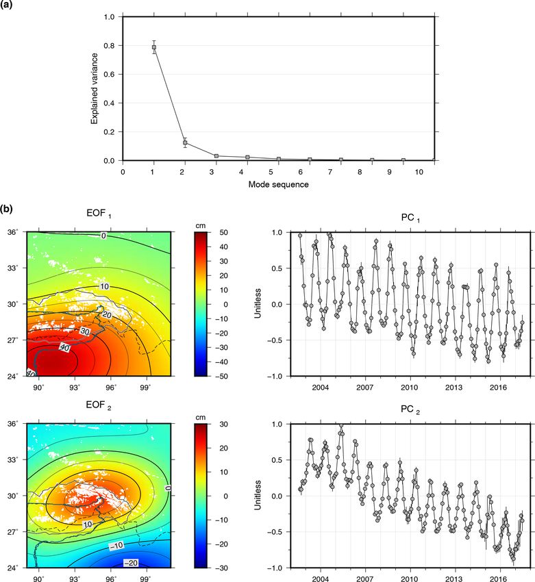
S. Yi et al.: Implication for substantial meltwater contribution to the Brahmaputra                                                                    2269

Figure 1. Geographic environment of the upper Brahmaputra basin. The boundary of the basin is outlined by the dashed black line. The
violet areas in the plateau represent mountain glaciers, but only the darker ones (9679 km2 in total) are studied here. The background colour
shows the amplitudes of annual variation in terms of equivalent water height from GRACE, and their peak months (the month with the peak
value in a year) are indicated using contours (e.g. 9 means September). The red triangles mark the locations of four meteorological stations.
The coloured arrows illustrate major climatic factors influencing this region (M: Indian monsoon; W: westerly winds; V: Bay of Bengal
vortex). The red box in the inset marks the location of the study area.

Table 1. Previous model-based estimates of meltwater contribution to the Brahmaputra discharge.

                                                                                                    Amount of
                                                                                Drainage             meltwater     Total discharge   Meltwater/total
             Study literature                               Time span         area (km2 )       (km3 w.e. yr−1 )       (km3 yr−1 )    discharge (%)
             Immerzeel et al. (2010)                      2000–2007              525 797                     62               230                27
             Bookhagen and Burbank (2010)                 1998–2007              255 929                     55               161                34
             Zhang et al. (2013)                          1961–1999             201 200a                     20                58                35
             Lutz et al. (2014)                           1998–2007              360 000                     43               131                33
             Huss et al. (2017)                          2002–2011b              533 000                    138               732                19
             Chen et al. (2017)                           2003–2014             240 000a                     12                60                21
         a Excludes large parts of the NTM region. b The time spans vary a bit in different datasets.

nals are further compared to the results of other datasets to                               the GeoForschungsZentrum (GFZ) in Potsdam and the Jet
validate their physical meanings. Such high-time-resolution                                 Propulsion Laboratory (JPL). These datasets are available at
observations also allow us to compare GS mass variations                                    http://icgem.gfz-potsdam.de (last access: 9 July 2020). The
with temperature records during the ablation season and to                                  degree 1 terms, which are absent in original GRACE re-
study the sensitivity of GS mass change in response to tem-                                 leases, have been added based on the technique proposed by
perature change. Finally, we will compare our results to pre-                               Swenson et al. (2008). The C20 terms have been replaced by
vious estimates at monthly, annual and interannual scales.                                  those from satellite laser ranging (Cheng et al., 2011), which
                                                                                            are considered to be more reliable. A widely used glacial iso-
                                                                                            static adjustment (GIA) model by A et al. (2013) is adopted
2     Data                                                                                  to correct the GIA effect caused by historical polar-ice-sheet
                                                                                            changes.
2.1    GRACE data and preprocessing                                                            Two different filtering strategies, a combination of a
                                                                                            P4M6 decorrelation (Swenson and Wahr, 2006) and 300 km
We adopt the monthly GRACE spherical harmonics Re-                                          Gaussian filter (hereafter G300 + P4M6) and a DDK4 filter
lease 06 products from August 2002 to June 2017. The three                                  (Kusche et al., 2009), are applied separately. Therefore, there
datasets are solved respectively by three organizations: the                                are six combinations, and their average values (with uniform
Center for Space Research (CSR) at the University of Texas,                                 weights) are used in the following figures.

https://doi.org/10.5194/tc-14-2267-2020                                                                            The Cryosphere, 14, 2267–2281, 2020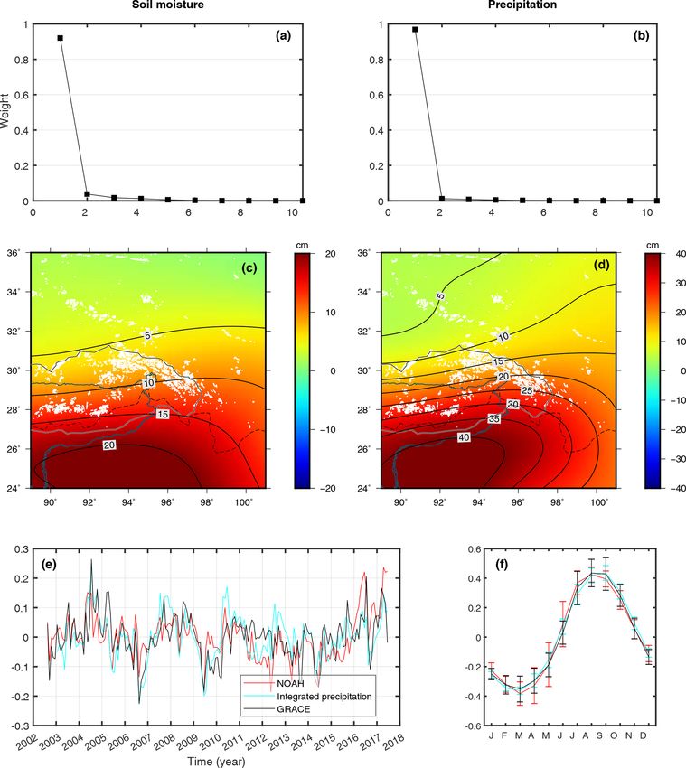
2270                                    S. Yi et al.: Implication for substantial meltwater contribution to the Brahmaputra

2.2    GRACE error estimation                                       glaciers are identified based on Randolph Glacier Inventory
                                                                    (RGI) 6.0 glacier outlines. (3) For each ICESat footprint,
We adopt different uncertainty estimation strategies for the        Shuttle Radar Topography Mission (SRTM; Farr et al., 2007)
seasonal variation and the trend due to their intrinsically dif-    elevations and slopes are extracted by bilinear interpolation
ferent error sources. The error in seasonal variation consists      of the digital-elevation-model grid cells. Glacier height vari-
of the standard deviations among these six datasets (i.e. er-       ation is defined as the elevation differences between the foot-
rors from the data solution and smoothing methods) and the          prints and the SRTM data. (4) We exclude footprints over
leakage error, while that in the long-term trend also includes      SRTM voids, footprints with slopes higher than 30◦ and foot-
other potentially uncorrected signals. We assume that the ma-       prints with a height change larger than 100 m (which are at-
jority of the hydrological signal is captured by the first EOF      tributed to biases caused by cloud cover during the ICESat
mode. The leakage error is then determined by how effec-            acquisition). (5) We also discard the calibration campaign
tively the hydrological and GS signals are separated by the         L1AB (March 2003) and the incomplete campaign L2F (Oc-
EOF technique. Based on the modelled and recovered glacier          tober 2009). (6) Glacier height variations are averaged and
mass changes, their residuals are estimated to have a seasonal      interpolated along the altitude to alleviate the uneven sam-
variation of up to 11 % of the modelled glacier mass change         pling problem in space, and an uncertainty of 0.06 m yr−1
(refer to Sect. 3.2 in the Supplement), which is used to calcu-     (Kääb et al., 2012) is chosen to account for the uneven sam-
late the seasonal leakage error. We do not quantify or account      pling bias in time. The steps have been used in previous work
for potential hydrological (non-GS) signals in EOF mode 2.          (Wang et al., 2017) and have also been described in earlier
   For the long-term trend error, the three different solu-         studies (Gardner et al., 2013; Kääb et al., 2012). The foot-
tions and two smoothing techniques have a total effect of           print information is given in Fig. S2.
0.44 Gt yr−1 . There are potential errors from other signal            ICESat has shown good ability to estimate snow varia-
sources, like the glacial isostatic adjustment (GIA), Little Ice    tion in flat regions (Treichler and Kääb, 2017), but apply-
Age (LIA) and weather denudation. The GIA effect which              ing the same technique in mountainous areas with high ter-
originates from the polar regions has been corrected by A’s         rain heterogeneity is cumbersome. Therefore, here ICESat
GIA model (A et al., 2013), although its influence on the           is only used to estimate changes in glacier mass. Although
trend is as small as 0.02 Gt yr−1 . The main reason is that the     our GRACE estimate includes both glaciers and snow, the
spatial pattern of GIA is quite smooth, so it mainly influences     estimates by GRACE and ICESat are comparable in the
the first mode and rarely leaks into the second one. This fea-      late ablation season (i.e. the October–November campaign
ture is also applicable for other signal sources: unless they       of ICESat), when the contribution of seasonal snow meltwa-
are exactly located in the glacierized area, their influence will   ter is negligible (Sect. 5.1). To convert the glacier thickness
be reduced by the EOF decomposition. In the southern and            changes into mass changes, two parameters are required, i.e.
southeastern Tibetan Plateau (over 500 000 km2 ), the effects       glacier density and total glacier area. We assume an average
of the LIA and denudation are estimated to be −1±1 Gt yr−1          glacier density of 850 ± 60 kg m−3 (Huss, 2013). According
(Jacob et al., 2012) and 1.6 Gt yr−1 (assuming the sediment         to the glacier inventory RGI 6.0 (RGI Consortium, 2017), the
has a density of 2 Gt km−3 ; Sun et al., 2009) respectively.        area has a glacierized area of 9679 km2 .
Our glacierized zone and surroundings have an area of about
100 000 km2 , accounting for one-fifth of the whole region, so      2.4   Other auxiliary data
we suppose their contribution to the GS mass estimate is also
proportionally one-fifth. However, as we explain above, we          To analyse the impact of temperature and precipitation on GS
could not precisely quantify their contribution without know-       and water mass balance here, we adopt two types of datasets,
ing their spatial distribution, and they are more likely to be      gridded reanalysis products and in situ measurements from
absorbed by the first mode, so we only include their contri-        four meteorological stations (their locations are labelled in
bution in the error estimation rather than correcting them in       Fig. 1, and coordinates are listed in Table S1 in the Sup-
the trend. Table 2 summarizes the sum of GRACE error esti-          plement). Precipitation and temperature records for each site
mates in the secular trend.                                         from 2003 to 2016 (Fig. S4) are available from the China
                                                                    Meteorological Data Service Center (http://data.cma.cn/data/
2.3    ICESat altimetry                                             weatherBk.html, last access: 9 July 2020). Only four in situ
                                                                    temperature records may not represent the overall condition
Version 34 of the ICESat Global Land Surface Altimetry              of the glacierized zone, so we adopt the gridded tempera-
Data is used to derive glacier height changes. The data span        ture product from the ERA5 reanalysis data processed by
is from 2003 to 2009, with two or three observation cam-            the European Centre for Medium-Range Weather Forecasts
paigns per year (Fig. S1 in the Supplement). The process-           (ECMWF). The data are available at https://www.ecmwf.int/
ing of ICESat data includes the following steps. (1) Or-            en/forecasts/datasets/reanalysis-datasets/era5 (last access: 9
thometric heights are obtained from original elevation data         July 2020). The gridded data are compared with station ob-
based on the Earth’s gravity model 2008. (2) Footprints of          servations, and the correlation index ranges from 0.69 to 0.82

The Cryosphere, 14, 2267–2281, 2020                                                    https://doi.org/10.5194/tc-14-2267-2020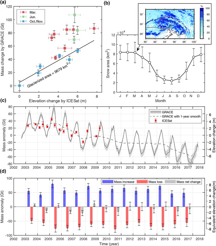
S. Yi et al.: Implication for substantial meltwater contribution to the Brahmaputra                                                      2271

Table 2. GRACE error sources for the long-term trend (Gt yr−1 ).

    Source                               Error   Remark
    Linear fit                           0.14    Calculated from fitting residuals of a linear and trigonometric model
    Data solution and smoothing errors   0.44    Estimated from the dispersion among CSR, GFZ and JPL with DDK4 and G300+P4M6
    Leakage error                        0.51    The average peak date may vary from 6 May to 16 May
    GIA                                  0.02    Difference between results with and without A’s GIA model (A et al., 2013)
    LIA                                  0.20    The total LIA effect in the whole Himalaya range and southeastern Tibet is −1 ± 1 Gt yr−1
    Denudation                           0.32    The total denudation effect in the eastern and southeastern Tibetan Plateau is 0.8 km3 yr−1
    Total                                0.78

in the interannual variation (Fig. S6), indicating a good con-            ized area studied here. Summer precipitation and its asso-
sistency. The average values in the glacierized zone from the             ciated hydrological mass change are enormous and well rec-
ERA5 temperature product will be used to represent the tem-               ognized, while the spring equivalents are not. Therefore, here
perature condition here.                                                  we only use the TRMM and ERA5 results from January to
   Global gridded precipitation data of the Tropical Rainfall             March in Fig. 2 to show the initiation of spring precipitation.
Measuring Mission (TRMM; Huffman et al., 2014) are used                   The precipitation begins to spread south and west starting
to examine the influence of precipitation on water storage.               in April, when the monsoon gradually increases (not shown
The data are available at https://pmm.nasa.gov/data-access/               here). The TRMM results show a boundary along the lat-
downloads/trmm (last access: 9 July 2020). Although such a                itude 29◦ N, where the precipitation suddenly decreases to
global product is unable to capture the localized spring pre-             the north. This boundary of change is irrelevant to the ter-
cipitation in our study area (Sect. 3), it can be used for the            rain and seems to be artificial. This phenomenon cannot be
investigation of large-scale monsoon precipitation.                       found in the ERA5 result, which shows abundant precipi-
   Moderate Resolution Imaging Spectroradiometer                          tation in the glacierized zone in these months. The bottom
(MODIS) data MOD10 (Hall et al., 2006) are used to                        plots give the GRACE monthly mass anomalies from March
investigate snow coverage here. The MOD10CM product                       to May (2 months later than the precipitation), as GRACE
has a temporal resolution of 1 month and spatial resolution of            observes the cumulative mass change resulting from precipi-
0.05◦ . The Global Land Data Assimilation System (GLDAS)                  tation. An earlier mass increase from April can be identified
Noah land surface model (Rodell et al., 2004) is adopted                  in the southeastern part of the Tibetan Plateau.
to inspect soil moisture changes, which can be compared                      The performance of TRMM and ERA5 is compared with
to changes in total terrestrial water storage estimated by                our station measurements in Fig. S5. According to the in situ
GRACE. Here, the version 2.1 monthly product with 1.0◦                    records, the spring precipitation, as a part of the bimodal vari-
spatial resolution is used (available at https://hydro1.gesdisc.          ation, is obvious at the Bomi and Chayu stations. TRMM
eosdis.nasa.gov/data/GLDAS/GLDAS_NOAH10_M.2.1/,                           is capable of revealing the conditions at Chayu at 28.65◦ N
last access: 9 July 2020). The total water storage in this                but performs poorly in regions north of 29◦ N. The ERA5
region also contains contributions from rivers and ground-                data demonstrate higher precipitation in winter and spring at
water, which are however difficult to obtain, so only the soil            Bomi and Linzhi than the other two datasets.
moisture component is investigated here.                                     These results show that spring precipitation can be cap-
                                                                          tured to a limited extent by various reanalysis products and
                                                                          the spring-accumulation pattern of GS mass change in the
3    Spring precipitation and mass increase                               SETP is recognizable in GRACE observations. The ampli-
                                                                          tude and phase of the seasonal mass variation from the equiv-
The method of this study is based on the fact that the                    alent water height (EWH) of GRACE are compared in the
change in GS mass driven by spring precipitation precedes                 background of Fig. 1. The seasonal amplitude has a spatial
the change in hydrological signals. Therefore, before intro-              distribution similar to that of the Indian-monsoon-affected
ducing the method, we want to demonstrate that GRACE                      area. This pattern reflects the predominance of the monsoon-
can detect mass changes caused by spring precipitation. At                controlled hydrological process and the weaker glacial sig-
two out of four stations (Bomi and Chayu), spring precipita-              nals in this region. However, the peak month of seasonal
tion is noticeable, even surpassing the summer–autumn pre-                changes (the contours in Fig. 1) divergently appears earliest
cipitation brought by the Indian monsoon (Fig. S4). Yang                  in June in the NTM and is gradually delayed to August in the
et al. (2013) provided precipitation records at 22 sites in a             southern Himalayas, where the annual amplitude reaches its
broader area and outlined the boundary of the impact zone                 maximum. The shift in peak months reflects the increasing–
of the spring precipitation, which roughly covers the glacier-            decreasing contribution from the sinusoid of the hydrological

https://doi.org/10.5194/tc-14-2267-2020                                                          The Cryosphere, 14, 2267–2281, 2020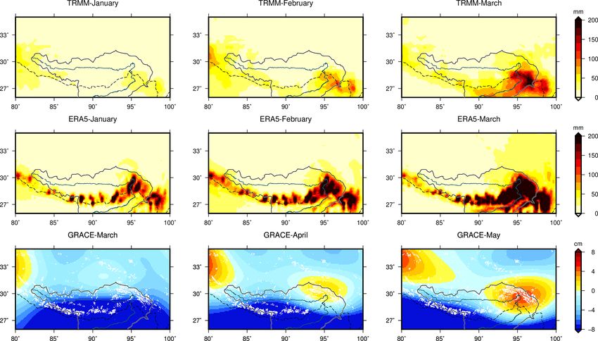
2272                                   S. Yi et al.: Implication for substantial meltwater contribution to the Brahmaputra

Figure 2. Monthly precipitation from January to March by TRMM and ERA5 and mass anomalies from March to May by GRACE. The
Brahmaputra and its basin boundary are marked. The white shaded areas in the bottom plots represent glacier distribution.

and GS seasonal variation. A key point to point out is that the   term changes (Fig. S7). Modes above mode 2 are weak and
peaks of hydrological and GS seasonal variations have a 3-        irregularly show much noise, so they are discarded here.
month time window offset (Sect. 4.4), which is a quarter of          The trends of the GRACE observation and its decomposed
the annual oscillation cycle and means that the two signals       modes are shown in Fig. 4. The GRACE observation shows
are mathematically orthogonal.                                    a significant mass loss, which is divided into the first two
                                                                  modes. In the glacierized zone, approximately two-thirds of
                                                                  the negative trend comes from the second mode and approx-
4     Decomposition of GRACE signals                              imately one-third comes from the first mode. The trend of
                                                                  higher modes (> 2) is quite weak (Fig. 4d).
4.1    EOF analysis of GRACE                                         According to the spatial coverages (EOF1 and EOF2 ) and
                                                                  their temporal variations (PC1 and PC2 ), the first mode cov-
GS and hydrological mass changes dominate the seasonal            ering the low altitude areas on the south of the plateau with a
gravity signals observed by GRACE in this region, and             peak month in August–September seemingly represents hy-
they are mathematically orthogonal due to different phases.       drologic signals and the second mode concentrating in the
Therefore, we employ the EOF technique (see the Supple-           glacierized region with a peak month in May (the peak month
ment for mathematic expressions; Björnsson and Venegas,           of June in Fig. 1 is the mixed result of the first two modes)
1997) to decompose hydrological and glacial signals in the        seemingly represents glaciers. We will verify these hypothe-
GRACE datasets (Fig. 3). We thus extract two modes with           ses below.
significantly higher explained variances than the other modes
(i.e. two significant modes are obtained). Results of different   4.2   GS mass estimation from mode 2
datasets and filters show good consistency, indicating that the
first two modes are robust.                                       GRACE results only show smooth mass patterns, and we
   Each mode consists of one EOF (the spatial pattern) and        need a strategy to recover the original amount of mass
one principal component (PC; the temporal evolution). Only        change. If we adopt the second mode to estimate GS
the first two modes, accounting for 79 %±5 % and 12 %±4 %         mass change, this step is necessary. Therefore, a forward-
respectively of the total variance explanation, are shown.        modelling method (Yi et al., 2016) is chosen to recover the
Although the first mode is much stronger than the second          mass in a predefined region iteratively. This method has been
mode (because the second one is more localized), their signal     widely used (Chen et al., 2015; Wouters et al., 2008), es-
strength in the glacierized region is comparable on both sea-     pecially in the study of polar ice sheets. In the first step,
sonal and secular temporal scales. Furthermore, after remov-      we divide the glacier mask based on the glacier distribution
ing the first mode representing the hydrological signal, mass     recorded in RGI 6.0 (RGI Consortium, 2017; Fig. 4e). The
changes in the glacierized zone estimated using the second        lattices have a resolution of 0.5◦ by 0.5◦ and are located in
mode of GRACE are much more consistent with the glacier           the glacierized area (in this way we assume the snow signal
mass changes using ICESat in terms of seasonal and long-          also comes from the glacierized area, but it does not influ-

The Cryosphere, 14, 2267–2281, 2020                                                  https://doi.org/10.5194/tc-14-2267-2020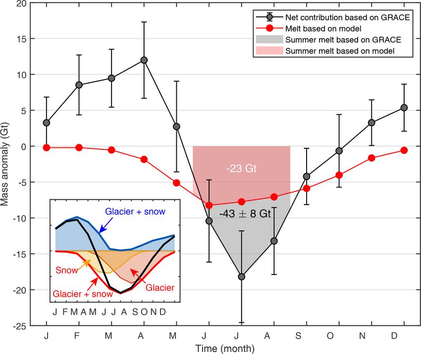
S. Yi et al.: Implication for substantial meltwater contribution to the Brahmaputra                                                2273

                                                                         interannual and seasonal scales as well. Note that precipita-
                                                                         tion is an instantaneous amount, while water storage is a state
                                                                         value, so the former should be integrated over time to make
                                                                         it comparable to the latter. Here, we integrate precipitation in
                                                                         6 successive months by an empirical weight function of (1,
                                                                         2, 3, 4, 5, 6), which will be normalized, and the value is at-
                                                                         tributed to the sixth month. Different integration methods are
                                                                         tested in the Supplement.
                                                                            Notably, mass contributions from the Brahmaputra river
                                                                         and groundwater are absent (and they are troublesome to ob-
                                                                         tain) and precipitation is assumed as the dominant driver of
                                                                         water storage change without considering the influence of
                                                                         runoff and evaporation (Humphrey et al., 2016), so we do
                                                                         not expect that we can reach a thorough agreement between
                                                                         different datasets. This is acceptable if their temporal consis-
                                                                         tency is targeted. However, long-term trends in runoff, evap-
                                                                         oration and groundwater cannot be ignored and they are dif-
                                                                         ferently reflected in these three products, so their trends have
                                                                         been removed before the comparison. The exclusion of un-
                                                                         available surface water and groundwater in the GLDAS re-
                                                                         sult also causes a weaker strength of its EOF1 compared to
                                                                         that of GRACE. We conclude that these datasets should be
Figure 3. EOF decomposition of GRACE observations in the form
                                                                         comparable in terms of seasonal and interannual variations
of EWH in the study region. Six combinations are averaged to gen-        and the pattern of spatial distribution but not in terms of the
erate these plots, and uncertainties are estimated based on the dis-     long-term trend and the amplitude of the spatial distribution.
persions. (a) Weight of the first 10 components. (b) Spatial distribu-   The good resemblance in both the EOF1 (spatial pattern) and
tion (EOF) and temporal variation (PC) in the first two components.      PC1 (seasonal and interannual temporal evolution) between
The white shaded areas represent glacier distribution.                   GRACE, GLDAS Noah and TRMM indicates that they re-
                                                                         flect similar geophysical processes, i.e. hydrological varia-
                                                                         tions.
ence the total mass estimates). In the second step, the mass
in each lattice is iteratively adjusted until its smoothing sig-         4.4   Method feasibility and reliability
nal (Fig. 4f) matches the GRACE observation (Fig. 4c) and
becomes stable. The details of each combination of datasets              The phase difference of 3 months is a prerequisite for this
and filters are presented in Figs. S8 and S9. Therefore, we              method and can be verified retrospectively. We tested differ-
estimate the mass in each combination (Fig. S9). The mass is             ent phase differences between hydrological and GS signals
multiplied by the PC2 series to derive the glacier mass series,          and decomposed them by the EOF method (refer to Sect. 3.1
and their average is taken as the mass estimate, which will be           in the Supplement). Only when the GS mass change peaks
compared with ICESat observations to test our hypothesis on              in May (3 months before the peak month of the hydrologi-
the estimate’s physical meaning.                                         cal signal) does our simulated result show similarities to the
                                                                         GRACE observation.
4.3   Validation of mode 1 by soil moisture and                             Only hydrological and GS signals can explain the first
      precipitation datasets                                             two modes considering their spatial and temporal patterns.
                                                                         The atmosphere contribution has already been removed in
To validate the hypothesis that the first mode represents hy-            GRACE observations (Dobslaw et al., 2017), and mass trans-
drological signals, we compare it with EOF decomposition                 ports of solid earth are unlikely to have such strong seasonal
results of two other datasets, soil moisture from GLDAS                  variations. We cannot quantify the contribution of groundwa-
Noah and precipitation data from TRMM (Fig. 5). To make                  ter in the second mode, but groundwater is apt to be mod-
them comparable to GRACE in terms of spatial resolution,                 ulated by stronger rainfall in summer (Andermann et al.,
they are expanded into spherical harmonics, truncated at de-             2012), rather than by snowfall in winter–spring, and ground-
gree 60, and smoothed by the same filter. Their results are              water activity will be reduced in winter–spring when the
shown in Fig. 5. Different from GRACE, which has two sig-                ground is frozen. Therefore, the groundwater component is
nificant modes, they each only have one due to the lack of               inclined to be captured by the first mode. We attribute the
a glacial signal. The EOF1 of GLDAS Noah and TRMM is                     negative trend in the first mode to decreasing precipitation
consistent with that of GRACE. The PCs are compared at                   in recent years (Fig. S10) and intense groundwater pumping

https://doi.org/10.5194/tc-14-2267-2020                                                       The Cryosphere, 14, 2267–2281, 2020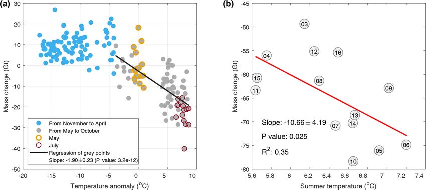
2274 S. Yi et al.: Implication for substantial meltwater contribution to the Brahmaputra
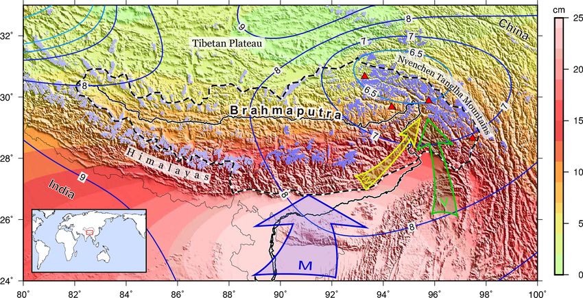
Figure 4. Trend of GRACE signals and the GS mass estimation. The CSR product with the DDK4 filter is used here. (a) The trend of
GRACE EWH observations between August 2002 and June 2017 is decomposed into (b), (c) and (d). Using the mass changes shown in (e),
we obtained (f) by the forward-modelling method to reproduce (c). The white shaded areas represent glacier distribution. The solid black
curve marks the basin boundary, and the dashed curve marks the plateau boundary.
(Shamsudduha et al., 2012). The negative trend in the second mass is not significant. The observations in March and June,
mode is supposed to represent GS melting and can be used as expected, are well above the line, implying an extra snow
for estimating GS mass balance. mass contribution, which can be inferred from the point-to-
line vertical distance. The snow contribution relative to the
total mass anomalies varies drastically between 0 % and 62 %
5 Results and discussion with a mean value of 38 % within our observation time win-
dows.
5.1 Glacier and snow mass balance The difference between GRACE and ICESat-based esti-
mates of mass change indicates that the snowpack outside the
The glacier surface elevation changes measured by ICESat glaciers is a non-negligible contributor to the seasonal mass
are compared with the result estimated from the second mode variation. This is quite different from previous glacier trend
of GRACE. We interpolate the series of GRACE estimates estimates, where non-glacier snow was neglected. Based
(2002–2017) into the observation epochs of ICESat (2003– on MODIS observations, the snow coverage area in this
2009) and plot mass changes by GRACE as a function of region varies from approximately 80 000 km2 in winter to
elevation changes by ICESat (Fig. 6a). After dividing by the 30 000 km2 in summer, both of which are much larger than
glacier density, the slope of the elevation–mass regression the inventoried glacier area (Fig. 6b). However, heteroge-
line represents the inventorial glacierized area by RGI 6.0. neous snow depths (Das and Sarwade, 2008) and densities
The observations in October–November (blue squares) ap- across the vast and rugged area make it difficult to measure
proximate with the line, indicating the good consistency be- their mass change in a non-gravimetric way.
tween ICESat and GRACE in the late ablation season be- Figure 6c compares the time series of glacial mass in the
tween 2003 and 2009. The MODIS result indicates that the SETP from GRACE (August 2002–June 2017) and ICESat
snow coverage increases rapidly from September (Fig. 6b), (2003–2009). The times series from two sensors are consis-
while the GRACE PC2 series show a moderate increase after tent in seasonal and interannual variations, despite the ab-
October. We speculate that the snow height does not increase sence of the snow component in the ICESat result. Monthly
much in the first few months, so the contribution of snow
The Cryosphere, 14, 2267–2281, 2020 https://doi.org/10.5194/tc-14-2267-2020S. Yi et al.: Implication for substantial meltwater contribution to the Brahmaputra 2275 Figure 5. EOF analysis of soil moisture using GLDAS Noah (a, c) and of precipitation using TRMM (b, d). The weights of the first 10 modes are shown in the upper panels (a, b). The first EOFs and PCs are shown in the middle and bottom panels (c–f). The PCs are separated into detrended interannual (e) and annual (f) variations for better comparison. mass change shows that the ablation season is generally be- with an average of −64.5 ± 8.9 Gt, and the annual mass tween June and October with slightly varied initiation and increase ranged from 41.8 to 79.9 Gt with an average of duration from year to year. The maximum mass increase (10– 58.6 ± 11.0 Gt. The seasonal GS mass changes postpone the 20 Gt) usually occurs in April, when the spring precipitation runoff of ∼ 60 Gt of winter–spring solid precipitation for sev- peaks, and the severest mass loss (−15 to −30 Gt) usually eral months. This amount plays a vital role in the annual occurs in July when the temperature peaks. As the tempera- streamflow (130.7 Gt on average) of the upper Brahmapu- ture rises from April to July, the monthly mass change curve tra (Lutz et al., 2014) and is almost 10 times the annual net drops steeply from the peak down to the trough, but the as- meltwater. Without the buffering effect of the seasonal varia- cending process with mass accumulation is relatively moder- tion, there will be a tremendous reduction in the streamflow ate and continuous. in summer and autumn, when the water demand is high, and We calculate annual mass increase and decrease by the dif- adaptive management on the dams in the Brahmaputra will ference in mass anomalies between November and May and be required to reduce seasonal irregularities in the stream- between June and October respectively. From 2002 to 2017, flow (Barnett et al., 2005). the annual mass decrease ranged from −49.3 to −78.3 Gt https://doi.org/10.5194/tc-14-2267-2020 The Cryosphere, 14, 2267–2281, 2020
2276                                    S. Yi et al.: Implication for substantial meltwater contribution to the Brahmaputra

Figure 6. GS mass balance in the SETP. (a) GS mass change by GRACE as a function of elevation change from ICESat. The values are
anomalies relative to the minimum in October 2007. (b) Seasonal snow coverage changes. The error bars are calculated by the dispersions
in the same month in the years from 2003 to 2016. The coverage in March is given in the inset. The dashed red outline marks the region
used for the calculation of snow area. (c) Time series of GS mass change estimated by GRACE and glacier mass change by ICESat. The
glacierized area of 9679 km2 is used to convert thickness change into mass change. (d) Annual mass increase and decrease from 2003 to
2016 by GRACE.

5.2    Quantifying the sensitivity of glacier and snow melt           no correlation is found during the accumulation season (from
       to temperature                                                 November to April). The mass peaks around May, when ei-
                                                                      ther glacier accumulation or ablation could happen. The tem-
                                                                      perature averaged in this transitional month is taken as the
Temperature is a dominant factor influencing the melting of           reference for the temperature anomalies used in the figure,
glaciers (Cogley et al., 2011, pp. 68). Here, the monthly tem-        and their mass changes are annotated. The highest sensitiv-
perature records from the ERA5 product are compared with              ity of monthly mass changes in response to temperature is
month-to-month mass changes by GRACE to investigate the               observed in July (3.1 ± 2.5 Gt per degree), when the largest
sensitivity of the GS mass balance in response to temperature         monthly mass loss occurs.
change (Fig. 7). Mass changes are negatively correlated with             To investigate the impact of climatic variables on the in-
the temperature anomalies by a factor of −1.9 ± 0.2 Gt per            terannual variations in GS mass, we compare annual mass
degree during the ablation season (from May to October), but

The Cryosphere, 14, 2267–2281, 2020                                                       https://doi.org/10.5194/tc-14-2267-2020
S. Yi et al.: Implication for substantial meltwater contribution to the Brahmaputra 2277
Figure 7. Regression between mass change and temperature. (a) Monthly mass changes as a function of monthly temperature anomalies.
(b) Linear regression between annual mass decreases and summer temperatures. The number in the circle represents the year of the data (e.g.
“15” is 2015).
losses (from May to October) with summer temperatures trend of GS mass change in this study by using GRACE is
(from June to August; Fig. 7b). The annual mass loss is sig- −6.5±0.8 Gt yr−1 between August 2002 and June 2017. The
nificantly correlated with the summer temperature, with a mass contribution from snow is considerable at the seasonal
slope of −10.7±4.2 Gt per degree (P value, 0.025; R 2 value, scale but negligible over 15 years, so the secular trend by us-
0.35), indicating that the annual GS mass balance is sensi- ing GRACE mainly represents the glacier mass change. Our
tive to summer temperature. The small value of R 2 is partly GRACE trend compares well with the derived glacier mass
due to the relatively large uncertainties in our mass estimate change of −5.5 ± 2.2 Gt yr−1 by using ASTER (the area-
(10 Gt) in this modest range of variation (30 Gt) and the ne- averaged rate in NTM and Bhutan multiplied by the glacier-
glect of other factors influencing GS mass balance. The sen- ized area of 9679 km2 ). In conclusion, both of our ICESat
sitivity index was provided by a previous study (Sakai and and GRACE estimates agree well with the previous ASTER
Fujita, 2017), where the whole HMA was examined and the result in terms of the secular trend. The GS mass trend from
SETP shows a widespread high sensitivity with an average the second mode is reduced by 25 % compared to the original
value of −1.23 m w.e. per degree. Based on the glacierized GRACE signal in the glacierized zone (Fig. 4).
area of 9679 km2 , our estimation is −1.10 ± 0.43 m w.e. per A recent result on changes in interannual glacier flow in
degree, which is comparable with the earlier study of Sakai this region (Dehecq et al., 2018) indicates a strong correla-
and Fujita (2017). It should be pointed out that annual net tion between ice flow rate and changes in glacial thickness.
mass balance was used in Sakai and Fujita (2017) in compar- The interannual variation in GRACE-based mass changes
ison with the annual mass loss used in this study, although (the 1-year smoothed sequence in Fig. 6c) notably shows
annual net mass balance is mainly driven by summer melt equilibrium during the periods of 2003–2005 and 2011–
(Ohmura, 2011). 2014. According to the aforementioned study (Dehecq et al.,
We could not find a significant relationship between the 2018), thinning glaciers reduce their flow rate by weaken-
mass and precipitation changes, probably because our data ing gravitational driving stress; therefore, this balanced mass
fail to reflect the strong orographic effect in precipitation state may slow down the decreasing flow rate. Coinciden-
and/or because the GS mass gain process is too complex to tally, we can identify such decelerating phases in the decline
be attributed to precipitation alone. in glacier flow rate during 2004–2006 and 2012–2015 (Fig. 1
in Dehecq et al., 2018).
5.3 Comparison with previous estimations on glacier GS mass loss is caused by flow, melting, and evaporation
and snow meltwater processes, and the last one does not contribute to the river
flow. Evaporation is important for continental-type glaciers
The trend of glacier elevation change by ICESat in this study where the climate is usually cold and dry. For example, it ac-
is −0.65±0.20 m w.e. yr−1 during 2003–2009, which lies be- counts for 12 % of the glacier ablation in Tianshan (Ohno et
tween the values of −0.30 ± 0.07 m w.e. yr−1 (Gardner et al., al., 1992). However, the importance of evaporation is greatly
2013) and −1.34 ± 0.29 m w.e. yr−1 (Kääb et al., 2015) in reduced in our maritime glaciers due to the extremely humid
eastern NTM by using a similar ICESat dataset (but an older air and rapid melting. Therefore, we assume that the mass
version) and is close to the trend of −0.62 ± 0.23 m w.e. yr−1 loss is completely turned into meltwater and can be com-
during 2000–2016 by using ASTER (Brun et al., 2017). The
https://doi.org/10.5194/tc-14-2267-2020 The Cryosphere, 14, 2267–2281, 20202278 S. Yi et al.: Implication for substantial meltwater contribution to the Brahmaputra
pared with analogous outputs from models. In our study re-
gion, 85 % of its meltwater (estimated according to the area
proportion) runs into the Brahmaputra, and this area accounts
for 83 % of total glaciers in this basin (9912 km2 ). Assuming
that the unobserved 17 % of glaciers have a similar rate of GS
mass change, our estimate of mass change is scaled by a ratio
of 1 × 0.85/0.83 = 1.02 to represent the GS mass change in
the entire Brahmaputra basin. Monthly changes in meltwater
estimated by month-to-month difference in GRACE results
are compared with model results of Lutz et al. (2014), which
showed that GS melt constitutes 33 % of the total discharge
in the Brahmaputra and that 50 % of the annual melt occurs
in the summer (Fig. 8). GRACE only detects the net change
in GS and cannot separate mass ablation and accumulation
(see the inset in Fig. 8). Because these two processes con-
cur simultaneously in transitional seasons and are offset to
some extent, the annual mass decrease (total mass loss in a
year; here, it ranges from 49.3 to 78.3 km3 with an average
Figure 8. Monthly mass change from GS in the upper Brahmaputra
of 64.5 km3 ) is smaller than the real GS melt. As a result,
basin estimated by GRACE and by the model of Lutz et al. (2014).
the annual mass decrease provides a lower bound on annual Negative values mean a net increase in meltwater (i.e. more GS melt
GS melt each year, rather than an accurate estimate. Instead, than accumulation). Note that Lutz’s model only estimated the melt
the amount of GS melt can be better determined during the component, while GRACE detects the net change including both
summer (from June to August), when the accumulation is melt and accumulation. The estimates of summer melt are anno-
supposed to be small. This value can be used to validate the tated. A schematic diagram of seasonal mass balance is shown in
model output. Our result shows that the summer melt ranges the inset (blue text represents mass accumulation, red represents
from 37.3 to 62.9 km3 with an average of 51.6 km3 , which ablation, and the black curve represents the net change). Note 85 %
is over 100 % larger than the 23 km3 GS mass change given of the meltwater in our study region runs into the Brahmaputra,
in the model of Lutz et al. (2014; Fig. 8). Although extrap- and this amount comes from 83 % of the glacierized area in this
basin; we scale our result by 1 × 0.85/0.83 to be comparable with
olated mass changes for the undetected 17 % of glaciers and
the model estimate.
the neglected summer evaporation may reduce our estimates
of summer meltwater, they definitely cannot explain the dif-
ference of more than 100 %. Among all model estimates, the
model of Lutz et al. (2014) reported one of the largest pro- The second EOF mode of GRACE observations is attributed
portions of GS melt contribution (33 %) but still largely un- to changes in GS mass, which can be validated in the fol-
derestimated the amount of summer meltwater, according to lowing three steps. First, a simulation experiment shows
our estimate from satellite observations. that two signals with peaks in August and May can be de-
Our annual mass decrease (average 49.0 Gt) is still much composed unbiasedly by EOF. Second, the first decomposed
smaller than the 137 Gt of annual meltwater given by Huss mode shows consistent spatio-temporal patterns with the soil
et al. (2017). However, this larger value even exceeds the moisture and precipitation variations from the GLDAS and
annual streamflow of 130.7 km3 in the upper Brahmapu- TRMM data and thus can be reasonably attributed to hydro-
tra where all GS meltwater is included (Lutz et al., 2014). logical processes. Thirdly, the second mode of the GRACE
The upper streamflow at the Nuxia station (ahead of the signal with a peak in May temporally corresponds to the
main glacier supply area) is ∼ 60 km3 . Therefore, the dif- glacier and snow accumulation and ablation processes and
ference in streamflow between the main glacier supply area spatially coincides with the glacier distribution, which is also
is ∼ 70 km3 , and the annual meltwater is unlikely to exceed supported by the spring precipitation pattern observed by me-
this value, considering the additional contribution of precip- teorological stations. Glacier mass change measured by ICE-
itation. These values generally represent decadal averages at Sat is further adopted to compare with our GRACE-based
the beginning of this century (Table 1), and they are therefore GS estimates, and good agreement is reached in the ablation
comparable. season when the snow contribution is negligible. The ICESat
measurements also show that the seasonal glacier mass vari-
ation is large, which is consistent with our finding that GS
6 Conclusions mass change in this region peaks in May.
The GRACE-based GS mass balance not only shows a
In this study, we use GRACE gravimetry to estimate the GS long-term decreasing trend of −6.5 ± 0.8 Gt yr−1 , generally
mass balance in the SETP from August 2002 to June 2017. comparable with previous studies on glacier mass balance
The Cryosphere, 14, 2267–2281, 2020 https://doi.org/10.5194/tc-14-2267-2020S. Yi et al.: Implication for substantial meltwater contribution to the Brahmaputra 2279
in the SETP, but also newly reveals a strong seasonal vari- 2018YFD0900804).
ation which postpones a water supply of about 60 Gt from
winter and spring to summer and autumn. The high sensitiv- This open-access publication was funded
ity of glacier mass changes responding to temperature shows by the University of Stuttgart.
that warming climate will exert strong impacts on the glacier
and snow mass balance from two aspects. On the one hand,
under the current glacier condition, the increase in summer Review statement. This paper was edited by Bert Wouters and re-
viewed by Enrico Ciracì and four anonymous referees.
temperature will enhance the annual meltwater by a factor of
−10.7 ± 4.2 Gt per degree. On the other hand, the seasonal
meltwater will shift earlier and reduce its supply in summer
and autumn, which will potentially result in 10 times the
amount of annual glacier melting. Our estimates of monthly References
GS meltwater can also give an elaborate calibration on the
glacier accumulation and ablation processes in hydrological A, G., Wahr, J., and Zhong, S.: Computations of the vis-
and glaciological models of the Brahmaputra basin, which coelastic response of a 3-D compressible Earth to sur-
face loading: an application to Glacial Isostatic Adjustment
were barely calibrated by GS mass observations and diverged
in Antarctica and Canada, Geophys. J. Int., 192, 557–572,
largely in terms of the proportion of seasonal meltwater con- https://doi.org/10.1093/gji/ggs030, 2013.
tribution. Given the high vulnerability to warming tempera- Andermann, C., Longuevergne, L., Bonnet, S., Crave, A., Davy,
ture, the greater contribution of meltwater to the Brahmapu- P., and Gloaguen, R. : Impact of transient groundwater storage
tra streamflow than most model estimates indicates that its on the discharge of Himalayan rivers, Nat. Geosci., 5, 127–132,
water resource allocation will face ominous tension in the 2012.
future. Barnett, T. P., Adam, J. C., and Lettenmaier, D. P.: Po-
tential impacts of a warming climate on water avail-
ability in snow-dominated regions, Nature, 438, 303–309,
Data availability. The data that support this study are mostly pub- https://doi.org/10.1038/nature04141, 2005.
licly open, and their sources are indicated in the “Data” section. The Biemans, H., Siderius, C., Lutz, A., Nepal, S., Ahmad, B., Hassan,
meteorological data and the series of glacier mass balance estimates T., von Bloh, W., Wijngaard, R., Wester, P., Shrestha, A., and Im-
are available upon request to the corresponding author. merzeel, W.: Importance of snow and glacier meltwater for agri-
culture on the Indo-Gangetic Plain, Nat. Sustain., 2, 594–601,
https://doi.org/10.1038/s41893-019-0305-3, 2019.
Supplement. The supplement related to this article is available on- Björnsson, H. and Venegas, S.: A manual for EOF and SVD analy-
line at: https://doi.org/10.5194/tc-14-2267-2020-supplement. ses of climatic data, CCGCR Report, 97, 112–134, McGill Uni-
versity, Canada, 1997.
Bolch, T., Kulkarni, A., Kaab, A., Huggel, C., Paul, F., Cogley, J. G.,
Frey, H., Kargel, J. S., Fujita, K., Scheel, M., Bajracharya, S., and
Author contributions. SY conceived the study and conducted the
Stoffel, M.: The State and Fate of Himalayan Glaciers, Science,
calculations. SY and CS analysed the results and wrote the
336, 310–314, https://doi.org/10.1126/science.1215828, 2012.
manuscript. KH discussed and revised the manuscript. SK discussed
Bookhagen, B. and Burbank, D. W.: Toward a complete Himalayan
and suggested the experiment. QW processed the ICESat data. LC
hydrological budget: Spatiotemporal distribution of snowmelt
processed the MODIS data.
and rainfall and their impact on river discharge, J. Geophys. Res.,
115, F03019, https://doi.org/10.1029/2009jf001426, 2010.
Brun, F., Berthier, E., Wagnon, P., Kääb, A., and Treichler, D.:
Competing interests. The authors declare that they have no conflict A spatially resolved estimate of High Mountain Asia glacier
of interest. mass balances from 2000 to 2016, Nat. Geosci., 10, 668–673,
https://doi.org/10.1038/ngeo2999, 2017.
Chen, J. L., Wilson, C. R., Li, J., and Zhang, Z.: Reducing
Acknowledgements. Shuang Yi is supported by JSPS and the leakage error in GRACE-observed long-term ice mass change:
Alexander von Humboldt Foundation. Chunqiao Song is supported a case study in West Antarctica, J. Geodesys., 89, 925–940,
by the Strategic Priority Research Program of the Chinese Academy https://doi.org/10.1007/s00190-015-0824-2, 2015.
of Sciences and the National Key R&D Program of China. Chen, X., Long, D., Hong, Y., Zeng, C., and Yan, D.: Improved
modeling of snow and glacier melting by a progressive two-stage
calibration strategy with GRACE and multisource data: How
Financial support. This research has been supported by the JSPS snow and glacier meltwater contributes to the runoff of the Upper
KAKENHI grant (grant no. JP16F16328), the Alexander von Hum- Brahmaputra River basin?, Water Resour. Res., 53, 2431–2466,
boldt Foundation, the Strategic Priority Research Program of the https://doi.org/10.1002/2016WR019656, 2017.
Chinese Academy of Sciences (grant no. XDA23100102) and the Cheng, M., Ries, J. C., and Tapley, B. D.: Variations of the Earth’s
National Key R&D Program of China (grant no. 2018YFD1100101, figure axis from satellite laser ranging and GRACE, J. Geophys.
Res., 116, B1, https://doi.org/10.1029/2010jb000850, 2011.
https://doi.org/10.5194/tc-14-2267-2020 The Cryosphere, 14, 2267–2281, 20202280 S. Yi et al.: Implication for substantial meltwater contribution to the Brahmaputra Cogley, J., Hock, R., Rasmussen, L., Arendt, A., Bauder, A., Braith- Kääb, A., Berthier, E., Nuth, C., Gardelle, J., and Arnaud, waite, R., and Nicholson, L.: Glossary of glacier mass balance Y.: Contrasting patterns of early twenty-first-century glacier and related terms, IHP-VII technical documents in hydrology, mass change in the Himalayas, Nature, 488, 495–498, 86, UNESCO, Paris, , 2011. https://doi.org/10.1038/nature11324, 2012. Das, I. and Sarwade, R.: Snow depth estimation over north-western Kääb, A., Treichler, D., Nuth, C., and Berthier, E.: Brief Communi- Indian Himalaya using AMSR-E, Int. J. Remote Sens., 29, 4237– cation: Contending estimates of 2003–2008 glacier mass balance 4248, https://doi.org/10.1080/01431160701874595, 2008. over the Pamir–Karakoram–Himalaya, The Cryosphere, 9, 557– Dehecq, A., Gourmelen, N., Gardner, A. S., Brun, F., Goldberg, D., 564, https://doi.org/10.5194/tc-9-557-2015, 2015. Nienow, P. W., and Trouvé, E.: Twenty-first century glacier slow- Kaser, G., Großhauser, M., and Marzeion, B.: Contribution down driven by mass loss in High Mountain Asia, Nat. Geos., 12, potential of glaciers to water availability in different cli- 22–27, https://doi.org/10.1038/s41561-018-0271-9, 2018. mate regimes, P. Natl. Acad. Sci. USA, 107, 20223–20227, Dobslaw, H., Bergmann-Wolf, I., Dill, R., Poropat, L., and Flecht- https://doi.org/10.1073/pnas.1008162107, 2010. ner, F.: AOD1B Product Description Document for Product Re- Kusche, J., Schmidt, R., Petrovic, S., and Rietbroek, R.: Decorre- lease 06 (Rev. 6.1, October 19, 2017), GFZ, Germany, 2017. lated GRACE time-variable gravity solutions by GFZ, and their Farr, T. G., Rosen, P. A., Caro, E., Crippen, R., Duren, R., Hens- validation using a hydrological model, J. Geodesy, 83, 903–913, ley, S., and Roth, L.: The shuttle radar topography mission, Rev. https://doi.org/10.1007/s00190-009-0308-3, 2009. Geophys., 45, RG2004, https://doi.org/10.1029/2005rg000183, Lutz, A. F., Immerzeel, W. W., Shrestha, A. B., and Bierkens, M. 2007. F. P.: Consistent increase in High Asia’s runoff due to increasing Gardelle, J., Berthier, E., Arnaud, Y., and Kääb, A.: Region- glacier melt and precipitation, Nat. Clim. Change, 4, 587–592, wide glacier mass balances over the Pamir-Karakoram- https://doi.org/10.1038/Nclimate2237, 2014. Himalaya during 1999–2011, The Cryosphere, 7, 1263–1286, Matsuo, K. and Heki, K.: Time-variable ice loss in Asian high https://doi.org/10.5194/tc-7-1263-2013, 2013. mountains from satellite gravimetry, Earth Planet. Sci. Lett., 290, Gardner, A. S., Moholdt, G., Cogley, J. G., Wouters, B., Arendt, A. 30–36, https://doi.org/10.1016/j.epsl.2009.11.053, 2010. A., Wahr, J., and Paul, F.: A Reconciled Estimate of Glacier Con- Ohmura, A.: Observed Mass Balance of Mountain Glaciers and tributions to Sea Level Rise: 2003 to 2009, Science, 340, 852– Greenland Ice Sheet in the 20th Century and the Present Trends, 857, https://doi.org/10.1126/science.1234532, 2013. Surv. Geophys., 32, 537–554, https://doi.org/10.1007/s10712- Hall, D., Salomonson, V., and Riggs, G.: MODIS/Terra 011-9124-4, 2011. snow cover daily L3 global 500 m grid, Version 5, Boul- Ohno, H., Ohata, T., and Higuchi, K.: The influence of humidity der, Colorado USA: National Snow and Ice Data Center, on the ablation of continental-type glaciers, Ann. Glaciol., 16, https://doi.org/10.5067/63NQASRDPDB0, 2006. 107–114, https://doi.org/10.3189/1992AoG16-1-107-114, 1992. Huffman, G., Bolvin, D., Braithwaite, D., Hsu, K., Joyce, R., RGI Consortium: Randolph Glacier Inventory – A Dataset of and Xie, P.: Tropical Rainfall Measuring Mission (TRMM) Global Glacier Outlines: Version 6.0: Technical Report, Global (2011), TRMM (TMPA/3B43) Rainfall Estimate L3 1 month Land Ice Measurements from Space, Colorado, USA, Digital 0.25◦ × 0.25◦ V7, Greenbelt, MD, Goddard Earth Sci- Media, https://doi.org/10.7265/N5-RGI-60, 2017. ences Data and Information Services Center (GES DISC), Rodell, M., Houser, P. R., Jambor, U., Gottschalck, J., Mitchell, https://doi.org/10.5067/TRMM/TMPA/MONTH/7, 2014. K., Meng, C. J., Arsenault, K., Cosgrove, B., Radakovich, J., Humphrey, V., Gudmundsson, L., and Seneviratne, S. I.: Assess- Bosilovich, M., Entin, J. K., Walker, J. P., Lohmann, D., and Toll, ing Global Water Storage Variability from GRACE: Trends, Sea- D.: The Global Land Data Assimilation System, B. Am. Mete- sonal Cycle, Subseasonal Anomalies and Extremes, Surv. Geo- orol. Soc., 85, 381–394, https://doi.org/10.1175/bams-85-3-381, phys., 37, 357–395, https://doi.org/10.1007/s10712-016-9367-1, 2004. 2016. Sakai, A. and Fujita, K.: Contrasting glacier responses to recent Huss, M.: Density assumptions for converting geodetic glacier climate change in high-mountain Asia, Sci. Rep., 7, 13717, volume change to mass change, The Cryosphere, 7, 877–887, https://doi.org/10.1038/s41598-017-14256-5, 2017. https://doi.org/10.5194/tc-7-877-2013, 2013. Shamsudduha, M., Taylor, R., and Longuevergne, L.: Mon- Huss, M., Bookhagen, B., Huggel, C., Jacobsen, D., Bradley, R. S., itoring groundwater storage changes in the highly sea- Clague, J. J., Vuille, M., Buytaert, W., Cayan, D., Greenwood, sonal humid tropics: Validation of GRACE measurements G., Mark, B., Milner, A., Weingartner, R., and Winder, M.: To- in the Bengal Basin, Water Resour. Res., 48, W02508, ward mountains without permanent snow and ice, Earth’s Future, https://doi.org/10.1029/2011WR010993, 2012. 5, 418–435, https://doi.org/10.1002/2016EF000514, 2017. Sun, W., Wang, Q., Li, H., Wang, Y., Okubo, S., Shao, D., Liu, Immerzeel, W. W., Van Beek, L. P., and Bierkens, M. F.: Climate D., and Fu, G.: Gravity and GPS measurements reveal mass change will affect the Asian water towers, Science, 328, 1382– loss beneath the Tibetan Plateau: Geodetic evidence of in- 1385, https://doi.org/10.1126/science.1183188, 2010. creasing crustal thickness, Geophys. Res. Lett., 36, L02303, Jacob, T., Wahr, J., Pfeffer, W., and Swenson, S.: Recent contri- https://doi.org/10.1029/2008gl036512, 2009. butions of glaciers and ice caps to sea level rise, Nature, 482, Swenson, S. and Wahr, J.: Post-processing removal of corre- 514–518, https://doi.org/10.1038/nature10847, 2012. lated errors in GRACE data, Geophys. Res. Lett., 33, L08402, Jansson, P., Hock, R., and Schneider, T.: The concept of https://doi.org/10.1029/2005gl025285, 2006. glacier storage: a review, J. Hydrol., 282, 116–129, Swenson, S., Chambers, D., and Wahr, J.: Estimating geocen- https://doi.org/10.1016/S0022-1694(03)00258-0, 2003. ter variations from a combination of GRACE and ocean The Cryosphere, 14, 2267–2281, 2020 https://doi.org/10.5194/tc-14-2267-2020
You can also read