Search-Based Motion Planning for Performance Autonomous Driving (DRAFT)
←
→
Page content transcription
If your browser does not render page correctly, please read the page content below

Search-Based Motion Planning
                                                     for Performance Autonomous Driving (DRAFT)

                                                                       Zlatan Ajanovic1∗ , Enrico Regolin2∗ ,
                                                               Georg Stettinger1 , Martin Horn3 and Antonella Ferrara2
arXiv:1907.07825v1 [cs.RO] 18 Jul 2019

                                                                         1Virtual Vehicle Research Center, Austria,
                                                             {zlatan.ajanovic, georg.stettinger}@v2c2.at,
                                                 2   Dipartimento di Ingegneria Industriale e dell’Informazione, University of Pavia, Italy,
                                                             enrico.regolin@unipv.it, a.ferrara@unipv.it
                                                        3 Graz University of Technology, Austria, martin.horn@tugraz.at

                                         Keywords: autonomous vehciles, trail-braking, drifting, motion planning

                                                     Abstract. Driving on the limits of vehicle dynamics requires predictive planning
                                                     of future vehicle states. In this work, a search-based motion planning is used to
                                                     generate suitable reference trajectories of dynamic vehicle states with the goal
                                                     to achieve the minimum lap time on slippery roads. The search-based approach
                                                     enables to explicitly consider a nonlinear vehicle dynamics model as well as con-
                                                     straints on states and inputs so that even challenging scenarios can be achieved in a
                                                     safe and optimal way. The algorithm performance is evaluated in simulated driving
                                                     on a track with segments of different curvatures.

                                         1 Introduction
                                         Similarly to other autonomous systems, autonomous vehicle control is based on a Sensing-
                                         Planning-Acting cycle. Predictive planning of future vehicle states can enable real-time
                                         control of driving while avoiding static obstacles [1] and can be extended to racing sce-
                                         narios with multiple agents (although not real-time) [2]. However, this Motion Planning
                                         (MP) approach is based on an exhaustive search and works well only for short horizons
                                         (due to exponential complexity) and in high friction conditions (where fast transitions be-
                                         tween simple, constant velocity primitives can be achieved). Approaches like this cannot
                                         be used for controlling a vehicle in lower friction conditions, which require larger hori-
                                         zons and a more detailed vehicle model as the control action often enters the saturated
                                         region.
                                            Another line of work considers this kind of situations, i.e. driving with high side-slip
                                         angles like drifting, trail-braking, etc. Most of the current work in this direction consid-
                                         ers sustained drift or transient drift scenarios. One example of a transient drift scenario
                                         is drift parking, as shown in [3], where the vehicle enters temporarily a drift state. On
                                         the other hand, in sustained drift scenarios, the goal is to maintain steady-state drifting.
                                         Velenis et al. modeled high side-slip angle driving and showed that for certain boundary
                                         conditions it can be a solution for the minimum-time cornering problem [4], [5]. Tav-
                                         ernini et al. showed that aggressive drifting maneuvers provide minimum time cornering
                                             ∗ Equal     contributions. Ajanovic focused on algorithmic while Regolin on vehicle dynamics
                                         part.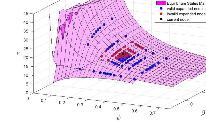
NOTICE: this is the authors’ version of the work that was accepted for publication in proceedings
of the IAVSD 2019 conference.

in low-friction conditions [6]. Because of computational complexity, most of these works
cannot achieve online performance.
   Based on results generated offline, by using [5], You and Tsiotras proposed a solution
for the learning of primitive trail-braking behavior, enabling online generation of trail-
brake maneuvers [7]. This approach decomposes trail-braking into three stages: entry
corner guiding, steady-state sliding and straight line exiting. A similar decomposition of
the problem was also presented in [8]. This one divides the horizon into three regions,
finds a path for each region and then concatenates them. As it appears from the results,
though, in the drifting region the rule-based solution produces non optimal solutions.
Impressive demonstration of model-based reinforcement learning approach on scaled
vehicle is shown in [9], however, as for the aforementioned sustained drift approaches,
considered scenario is relatively simple with only one curve. It is hard to expect that these
approaches generalize well to more complicated scenarios. Driving the full track gener-
ally requires solving more curves, with variable curvature radius and a mix of right and
left curves. In this scenario the “three-segments” assumption does not hold, and finding
out how to split the horizon and assigning the segments arises as a problem, which can
be viewed as a combinatorial optimization problem. This confirms that the problem of
continuous driving is a different one from sustained drift or transient drift.
   As generating references in a continuous driving problem can be considered as a com-
binatorial optimization problem, heuristic search methods like A∗ can be effectively used
for automated optimal trajectory generation. In this paper, a novel A∗ search-based ap-
proach to the problem of generating “trackable” references is presented. The presented
A∗ search-based planner is a modified version of the one illustrated in [10], where a rather
simple vehicle model was used to generate vehicle trajectories in complex urban driving
scenarios. The space of the possible trajectories is explored by expanding different combi-
nations of motion primitives in a systematic way, guided by a heuristic function. Motion
primitives are generated using two different vehicle models. A bicycle model is used
for small side-slip angle operations (i.e. entry and exit maneuvers and close-to-straight
driving) and a full nonlinear vehicle model for steady state cornering maneuvers. Such
automated motion primitives generation enables to generate arbitrary trajectories, not
limited to just one curve as in previous approaches.
   The presented expansion approach is similar to the closed-loop prediction approach
(CL-RRT) [11], which uses closed-loop motion primitives for the expansion when open-
loop dynamics are unstable, so that the exploration by variations in the open-loop dynam-
ics becomes inefficient. In our approach, we expand steady state cornering motion primi-
tives, which are considered to be achievable via closed-loop control such, as in e.g. [12].

2 Problem Formulation and Vehicle Models
The tackled problem in this work is minimum lap time driving on an empty track in low
friction conditions, i.e. gravel road. It is assumed that the vehicle is equipped with a map
of the road and a localization system. Therefore, the vehicle has the information about
the road ahead, as well as left/right boundaries and exact position and orientation. More-
over, the full vehicle state feedback information is available. In particular, besides dy-
namic states, the low level controller (which is not covered in this work) for state tracking
requires measurements and estimates of several quantities, including wheel forces and
wheel slips, both longitudinal and lateral (see e.g. [13]). Finally, the combined longitudi-
nal/lateral tire-road contact forces characteristics are assumed to be known and constant.
NOTICE: this is the authors’ version of the work that was accepted for publication in proceedings
of the IAVSD 2019 conference.

The road, on the other hand, is assumed to be flat, with static road-tire characteristic and
can have arbitrary shape with constant width.

2.1 Vehicle kinematic model
The vehicle trajectories are generated by concatenating smaller segments of trajectories,
the so-called "motion primitives". These are generated based on a model for the vehicle
planar motion. Such model is comprised of six states [x, y, ψ , v, β , ψ̇ ]T , where x, y and
ψ represent kinematic states (position and yaw angle), and v, β are vehicle velocity and
side-slip
      angle respectively. The evolution of x and y is given by:
        ẋ = v·cos(ψ + β )
                                                                                            (1)
        ẏ = v·sin(ψ + β )
whereas v, β , ψ̇ are given by the selected vehicle model.
   In regular driving situations, i.e. for small values of β , the trajectory identified by (1)
is mostly determined by v and ψ̇ , and therefore can be planned by means of linearized
vehicle models, valid for small variations of β and ψ̇ . When driving on slippery surfaces,
such solution is not suitable anymore, due to the effect of β in (1) and to the complex-
ity of the model which describes the vehicle motion for growing values of β . A major
limitation which stems from using a full nonlinear vehicle model is the so-called "curse
of dimensionality", and related computational explosion when introducing new states. In
fact, if motion primitives were generated with the full nonlinear vehicle model, the com-
putational burden would increase excessively, thus making it a non viable option for an
online implementation.
   To overcome unnecessary increase in computation, we generate motion primitives by
using: i) the so-called “bicycle model” [14] in straight-driving/mild-turning scenarios,
and ii) a convenient approximation of the full nonlinear model, based on the theoretical
vehicle-equilibrium-states during cornering.

2.2 Equilibrium States Manifold
For cornering, the motion primitives are generated based on previously computed vehicle-
equilibrium-states. When generating target reference states, one of the main issues is en-
suring that the reference values can be actually reached in a sufficiently short time. This
problem is made harder by the slow dynamics of the vehicle longitudinal and lateral ac-
celerations, due to the slippery surface considered. Two devices are exploited to counter
this problem: i) “slow varying” reference set-points are used, in order to allow the low
level actuator to bring the actual state in proximity of the desired one; ii) only reference
states belonging to a specific “Equilibrium States Manifold” (ESM) are considered. To
obtain such manifold, which requires a reliable model for vehicle and tire-road contact
forces, an off-line computation is performed, which provides the steady-state solutions of
the vehicle cornering at different curvature radii [15]. These solutions include the vehicle
control inputs (steering wheel angle and rear wheels slip) as well as the vehicle states v, β ,
ψ̇ . For the offline computation of the equilibrium points, the full-vehicle nonlinear model
is exploited, where the tire-road forces Fx ,Fy for each axle (Fx, f = 0 due to the RWD con-
figuration) are obtained from the normal forces Fz and the combined longitudinal/lateral
friction model (see [16]):
      Fx,i = Fz,i µx (λi ,αi ), Fy,i = Fz,i µy (λi ,αi )                                  (2)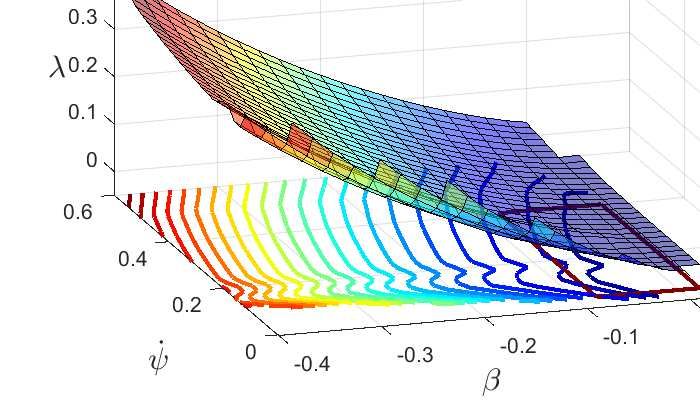
NOTICE: this is the authors’ version of the work that was accepted for publication in proceedings
of the IAVSD 2019 conference.
Fig. 1. Equilibrium points sets Sss (and linear interpolation) in the v, β , ψ̇ space for counter-
clockwise cornering maneuvers with different curvature radii Rc .
where µ is the friction coefficient, λ and α the longitudinal and lateral slips respectively.
The nonlinear friction functions take the form of the Magic Formula (MF) tire friction
model, with an isotropic friction model being used for simplicity. This requires the com-
putation of the theoretical slip quantities (σ j , j ∈ {x,y}), which can be obtained from α ,
λ as follows:
λ tanα q
σx = , σy = , σ = σx2 + σy2 (3)
1+ λ 1+ λ
Then, the one-directional friction coefficients are given by
σi
µi = Dsin[Cλ arctan{σ B−E(σ B−arctanσ B)}], (4)
σ
for i = x,y, with B = 1.5289, C = 1.0901, D = 0.6, E = −0.95084 being the Pacejka
parameters corresponding to gravel.
The vehicle responses can be obtained from the following system of nonlinear equa-
tions, which considers the lateral, longitudinal and rotating balance equilibrium equa-
tions around the vehicle center of gravity:
F
v̇ = ψ̇ vβ + mx,r
(5)
mv(β̇ + ψ̇ ) = Fy, f +Fy,r
Jz ψ̈ = l f Fy, f −lr Fy,r
where Jz is the vehicle inertia around the z-axis, m the vehicle mass and l f , lr are the dis-
tances of the vehicle COG from the front and rear axles respectively. In addition, also the
longitudinal weight transfer is considered. Assuming a RWD drivetrain configuration,
and given different sets of values of the constant control inputs (steering wheel angle
δ , driving wheels slip λ ) the equilibrium points Sss = [vss ,βss ,ψ̇ss ]T can be computed, in
order to achieve different constant curvature radii Rc, by considering the uniform circular-
motion relation ψ̇ = Rvc , and imposing in (5) the steady-state condition
v̇ = β̇ = ψ̈ = 0. (6)
In Fig. 1 these sets are graphically displayed in the 3-dimensional state-space, for varying
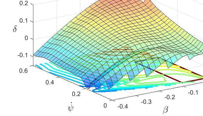
Rc . The corresponding surfaces, generated for δ and λ are displayed in Fig. 2.
NOTICE: this is the authors’ version of the work that was accepted for publication in proceedings
of the IAVSD 2019 conference.

Fig. 2. ESM for the inputs δ (left) and λ (right), counter-clockwise maneuvers. The highlighted
portion of the β − ψ̇ plane corresponds to the one in which the bicycle model representation is
considered valid. The intervals of values [δmin , δmax ], [λmin , λmax ] are used for the bicycle-model
expansion explained in Section 3.1.

   Let us assume that the tire-road contact model and the vehicle model (2)-(5) are correct,
and that a trajectory of any curvature radius Rc is given, for which at least one reference
state Sss (Rc ) exists. Then, if a locally stable feedback controller for the tracking of the
state is designed, such trajectory can be tracked, given an initial condition close enough
to the target state.
   A race track is composed of different sections, with varying curvature radii as well
as straight segments. Therefore, in order to determine the sequence of vehicle states to
be tracked by the vehicle, a continuous transition between different equilibrium points
would be required, neglecting condition (6). For this reason, the sets Sss (Rci ), i = 1,..,r
in Fig. 1 have been interpolated into a map v = f (β ,ψ̇ ), which represents the ESM from
which the sequences v,β ,ψ̇ which generate the trajectories are taken, the same procedure
being applied for δ , λ in Fig. 2.

2.3 Drivable road and Criteria

It is considered that the vehicle can drive only on the road R. Therefore, the drivability
of the trajectory generated based on the vehicle model is validated based on vehicle coor-
dinates x, y and yaw angle ψ only (not by higher dynamic states). To simplify planning,
the drivable road is modeled using a Frenet frame [17]. Instead of using x and y coordi-
nates, in Frenet frame one dimension represents the distance traveled along the road s,
and other the deviation from the road centerline d. In this way, to determine whether the
vehicle is on the road, it is sufficient to check the lateral deviation in Frenet frame. The
Frenet frame is only used for trajectory evaluation during planning, to ensure that the
planning procedure remains the same for each segment of the road. It is not used for the
underlying motion primitive generation, which is based on the vehicle dynamic model in
Euclidean space.
    As for the trajectory evaluation criteria, since the goal is to minimize lap time and plan-
ning horizon time is fixed, an equivalent behavior can be achieved by maximizing the
distance traveled along the road in a defined time horizon. The criteria can be evaluated
simply by considering the first coordinate in Frenet frame.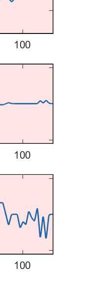
NOTICE: this is the authors’ version of the work that was accepted for publication in proceedings
of the IAVSD 2019 conference.

  Algorithm 1: A∗ Heuristic Search for a horizon
      input :nI , Obstacles data (O), h(n)
  1   begin
  2       n ←nI ,C LOSED ←∅,O PEN ←n                                       // initialization
  3       while n.k ≤ khor and O PEN 6= ∅ and O PEN.size() ≤ Ntimeout do
  4           n ←Select(O PEN)
  5           (n′ ,nC ) ← Expand(n, Children, ColCheck)
  6           C LOSED ← C LOSED ∪n∪nC ,O PEN ← O PEN \n∪n′
  7       return Path ()

3 Motion planning
The proposed Motion planning framework is based on the A∗ search method [18], guided
by an heuristic function in an MPC-like replanning scheme. After each time interval Trep ,
replanning is triggered from the current vehicle state, together with information about the
drivable road ahead.
   The trajectory is generated by a grid-like search using A∗ (see Algorithm 1). The grid
is constructed via discretization of the state variables x. Starting from the initial node (i.e.
state), chosen as the first current node, all neighbors are determined by expanding the
current node using motion primitives. The resulting child nodes are added to the O PEN
list. If the child node is already in the O PEN list, and the new child node has a lower cost,
the parent of that node is updated, otherwise it is ignored. From the O PEN list, the node
with the lowest cost is chosen to be the next current node and the procedure is repeated
until the horizon is reached, the whole graph is explored or the computation time limit
for planning is reached. Finally, the node closest to the horizon is used to reconstruct the
trajectory. To avoid rounding errors, as the expansion of a node creates multiple transi-
tions which in general do not end at gridpoints, the hybrid A∗ approach [19] is used for
planning. Hybrid A∗ also uses the grid, but keeps continuous values for the next expan-
sion without rounding it to the grid, thus preventing the accumulation of rounding errors.
Each node n contains 20 values: 6 indexes for each state in x (n.xk , n.yk , n.ψk , etc.), 6
indexes for the parent node (to reconstruct the trajectory), six remainders from the dis-
cretization of states (n.xr , n.yr , n.ψr , etc.), the exact cost-to-come to the node (n.g), and
the estimated total cost of traveling from the initial node to the goal region (n. f ). The
value n. f is computed as n.g+h(n), where h(n) is the heuristic function.
   The planning clearly requires processing time. The compensation of the planning time
can be achieved by introducing Tplan , a guaranteed upper bound on planning time. The
planning is then initiated from a position where the vehicle would be after the Tplan . The
old trajectory is executed while the new one is being processed. Thus, the new trajectory
is already planned when Tplan arrives. This approach has been widely used in MP for
automated vehicles [20].

3.1 Node expansion
To build trajectories iteratively, nodes are expanded and child nodes (final states on the
motion primitives) are generated, progressing towards the goal. From each node n, only
dynamically feasible and collision-free child nodes n′ should be generated. As mentioned
NOTICE: this is the authors’ version of the work that was accepted for publication in proceedings
of the IAVSD 2019 conference.
0.6
Bicycle
0.4
0.2 Both
ψ̇
0
-0.2 Surface
-0.4
No Exp.
-0.6
-0.6 -0.4 -0.2 0 0.2 0.4
β
(a) (b)
Fig. 3. (a) β − ψ̇ map representing the expansion modes depending on initial states. (b) Expanding
parent node n to different child nodes n′ on the ESM.
before, child nodes (motion primitives) are generated based on two models, bicycle
model for a close-to-straight driving and vehicle-equilibrium-states during cornering.
During cornering, the child nodes (motion primitives) are generated based on the
steady state dynamic states Sss , as explained in Section 2.2. Based on the current steady
state Sss , several reachable dynamic states are generated and (1) is used to simulate the
evolution of other states (x,y, ψ ) during the linear transition to these new steady states.
New steady states are obtained by sampling the β − ψ̇ space around the current value
(β0 , ψ̇0 ), with the density of the samples decreasing as the distance from the current po-
sition increases (see Fig. 3(b)). The number of evaluated samples is a tuning parameter,
which impacts considerably the performance of the search, as a trade-off between compu-
tation time and sufficient space exploration is needed. Since (6) assumes that the rate of
change of states is equal to zero, in order to generate trajectories which keep the vehicle
on the road, this constraint must be ’softened’.
In order to avoid generating and propagating an excessive amount of branches, before
the nodes which are in collision are removed, the following rules are considered: i) only
equilibrium points defined within the surface in Fig. 1 are considered, so that the mini-
mum reachable curvature radius is Rc,min = 10m; ii) the (small) portion of curve such that
β · ψ̇ > 0 is neglected, since in general equilibrium points in which β and ψ̇ share the
same sign are associated with low velocity conditions; iii) a maximum velocity deviation
∆ v between two successive nodes is defined, such that ∆ v/T s < amax , where amax is the
estimated maximum deceleration allowed on the given road surface.
Nodes are always expanded by “exploring” the neighboring states of the ESM. How-
ever, as illustrated in Fig. 3(a), when the current conditions are close enough to the origin
of the β − ψ̇ plane, i.e. for |β | < βlin and |ψ̇ | < ψ̇lin , also dynamic states and trajectories
generated according to a nonlinear bicycle model are considered, where the forces in (5)
are replaced with their linearized approximations
ψ̇ ψ̇
Fy, f = −C f (β +l f − δ ), Fy,r = −Cr (β −lr ), Fx,r = −Cx λ (7)
v v
In (7) the longitudinal and lateral stiffness coefficients Cx , C f , Cr are consistent with the
full characteristics given by (4). In order to generate the node expansions, the steeringNOTICE: this is the authors’ version of the work that was accepted for publication in proceedings of the IAVSD 2019 conference. Fig. 4. Graphical representation of the trajectories exploration in U-turn (left) and wide turn (right). wheel angle δ and the rear wheels slip λ are varied within the ranges defined by |β | < βlin and |ψ̇ | < ψ̇lin in the equilibrium surfaces in Fig. 2. 3.2 Heuristic function The heuristic function h(n) is used to estimate the cost needed to travel from some node n to the goal state (cost-to-go). As it is shown in [18], if the heuristic function is under- estimating the exact cost to go, the A∗ search provides the optimal trajectory. For the shortest path search, the usual heuristic function is the Euclidean distance. On the other hand, to find the minimum lap time, the heuristic should estimate the distance which the vehicle can travel from the current node during the defined time horizon. It is optimistic to assume that the vehicle accelerates (with maximum acceleration) in the direction of the road central line until it reaches the maximum velocity, and then maintains it for the rest of time horizon. Based on this velocity trajectory, the maximum travel distance can be computed and used as heuristic. Sacrificing optimality, in order to bias expansions towards the preferred motion and a better robustness, the heuristic function is augmented considering, among others: i) a “dynamic states evolution” cost, which helps limiting the rate of change of the references v, β , ψ̇ , in order to obtain smooth trajectories and facilitate state tracking; ii) penalization for trajectories approaching the road side; iii) penalization of the nodes with less siblings, thus biasing the search to avoid regions where only few trajectories are feasible. 4 Simulations The presented concept is evaluated in the Matlab/SIMULINK environment, assuming perfect actuation, i.e. the actual vehicle dynamical states/positions match the ones planned at the previous iteration. The trajectory exploration can be appreciated in Fig. 4in the case of a U-turn and of a wider curve. The explored branches are represented by the red links, and the closed nodes are marked as green. The light-blue car frames represent the optimal vehicle states (see Fig. 4). In Fig. 5(a) several frames of the same maneuver are shown (the top left turn in the track illustrated in Fig. 5(c)). From these, it is possible to appreciate how at each iteration the optimal trajectory is re-calculated based on the current position. Given the nature of the receding horizon approach, it is not guaranteed (nor preferred) that all or part of the previously computed trajectory are kept in the next iteration. In fact, while in the first
NOTICE: this is the authors’ version of the work that was accepted for publication in proceedings
of the IAVSD 2019 conference.

                            (a) U-turn maneuver: consecutive frames.

                                                     S5                     S6

                                                                                 S2

                                                             S4
                                                                                      S3       S1

                                                     50 m

      (b) Reference dynamical states.                       (c) Obtained driving trajectory.

            Fig. 5. Dynamical states and trajectory evolution over the full test-circuit.

step the trajectory ’dangerously’ approaches the side of the road, in the next two steps
the trajectory is incrementally regularized, thanks to the fact that the exploration of such
portion of the track is now being evaluated in earlier nodes.
   The dynamical states, which represent the output of the trajectory generation, are de-
picted in Fig. 5(b). One can see how the generated references are varied smoothly, in
particular in terms of v and β , which are the quantities characterized by slower actuation
dynamics. Moreover, it is possible to distinguish clearly 4 intervals in which the optimal
generated maneuver is a ’drift’ one with β > 0.4rad. These same intervals can be recog-
nized in Fig. 5(c), where the overall trajectory on the considered 10m-wide track can be
evaluated.

5 Conclusions

In this paper, a novel A∗ search-based motion planning for performance driving is pre-
sented and used to generate dynamically feasible trajectories on a slippery surface. The
proposed method extends drift-like driving from a steady state drifting on single curve to
a continuous driving on the road effectively entering and exiting drifting maneuvers and
switching between right and left turns. The proposed method assumes that the vehicle
parameters and the road surface properties are known to a certain degree, which allows
to define a set of steady-state cornering maneuvers. The method is evaluated on a mixed
circuit characterized by slippery conditions (gravel), which contains several road sec-
tions of varying curvature radii Rc . In several instances, due to the particular road surface
considered, the optimal selected trajectory involves drifting, which in certain conditions
ensures the maximum lateral acceleration. Such a result demonstrates the capability of
NOTICE: this is the authors’ version of the work that was accepted for publication in proceedings
of the IAVSD 2019 conference.
the proposed hybrid A∗ algorithm to generate feasible sub-optimal trajectories on slippery
conditions, while considering a limited prediction horizon. Moreover, when considering
U-turns with curvature radius as tight as 15m, such trajectories are comparable in shape
to the ones obtained when the full segment is optimized in order to find the minimum
time optimal maneuver, as in e.g. [6].
Acknowledgment
The project leading to this study has received funding from the European Union’s Horizon 2020 re-
search and innovation programme under the Marie Skłodowska-Curie grant agreement No 675999,
ITEAM project. VIRTUAL VEHICLE Research Center is funded within the COMET - Compe-
tence Centers for Excellent Technologies - programme by the Austrian Federal Ministry for Trans-
port, Innovation and Technology (BMVIT), the Federal Ministry of Science, Research and Econ-
omy (BMWFW), the Austrian Research Promotion Agency (FFG), the province of Styria and the
Styrian Business Promotion Agency (SFG). The COMET programme is administrated by FFG.
References
1. A. Liniger, A. Domahidi, and M. Morari, “Optimization-based autonomous racing of 1:43
scale rc cars,” Optimal Control Applications and Methods, vol. 36, no. 5, pp. 628–647, 2015.
2. A. Liniger and J. Lygeros, “A noncooperative game approach to autonomous racing,” IEEE
Transactions on Control Systems Technology, pp. 1–14, 2019.
3. J. Z. Kolter, C. Plagemann, D. T. Jackson, A. Y. Ng, and S. Thrun, “A probabilistic approach to
mixed open-loop and closed-loop control, with application to extreme autonomous driving,” in
2010 IEEE International Conference on Robotics and Automation. IEEE, 2010, pp. 839–845.
4. E. Velenis, P. Tsiotras, and J. Lu, “Modeling aggressive maneuvers on loose surfaces: The
cases of trail-braking and pendulum-turn,” in ECC. New York: IEEE, 2015, pp. 1233–1240.
5. ——, “Optimality properties and driver input parameterization for trail-braking cornering,”
European Journal of Control, vol. 14, no. 4, pp. 308–320, 2008.
6. D. Tavernini, M. Massaro, E. Velenis, D. I. Katzourakis, and R. Lot, “Minimum time
cornering: the effect of road surface and car transmission layout,” Vehicle System Dynamics,
vol. 51, no. 10, pp. 1533–1547, 2013.
7. C. You and P. Tsiotras, “Real-time trail-braking maneuver generation for off-road vehicle
racing,” in 2018 Annual American Control Conference (ACC). IEEE, 2018, pp. 4751–4756.
8. F. Zhang, J. Gonzales, S. E. Li, F. Borrelli, and K. Li, “Drift control for cornering maneuver
of autonomous vehicles,” Mechatronics, vol. 54, pp. 167–174, 2018.
9. G. Williams, N. Wagener, B. Goldfain, P. Drews, J. M. Rehg, B. Boots, and E. A. Theodorou,
“Information theoretic mpc for model-based reinforcement learning,” in 2017 IEEE
International Conference on Robotics and Automation (ICRA), May 2017, pp. 1714–1721.
10. Z. Ajanovic, B. Lacevic, B. Shyrokau, M. Stolz, and M. Horn, “Search-based optimal motion
planning for automated driving,” in 2018 IEEE/RSJ International Conference on Intelligent
Robots and Systems (IROS). IEEE, 2018, pp. 4523–4530.
11. Y. Kuwata, J. Teo, S. Karaman, G. Fiore, E. Frazzoli, and J. How, “Motion planning in
complex environments using closed-loop prediction,” in AIAA Guidance, Navigation and
Control Conference and Exhibit, 2008, p. 7166.
12. E. Regolin, M. Zambelli, and A. Ferrara, “A multi-rate ism approach for robust vehicle
stability control during cornering,” IFAC-PapersOnLine, vol. 51, no. 9, pp. 249–254, 2018.
13. E. Regolin, A. G. A. Vazquez, M. Zambelli, A. Victorino, A. Charara, and A. Ferrara, “A
sliding mode virtual sensor for wheel forces estimation with accuracy enhancement via ekf,”
IEEE Transactions on Vehicular Technology, vol. 68, no. 4, pp. 3457 – 3471, Apr. 2019.NOTICE: this is the authors’ version of the work that was accepted for publication in proceedings
of the IAVSD 2019 conference.
14. G. Genta, Motor vehicle dynamics: modeling and simulation. World Scientific, 1997, vol. 43.
15. E. Velenis, D. Katzourakis, E. Frazzoli, P. Tsiotras, and R. Happee, “Steady-state drifting stabi-
lization of rwd vehicles,” Control Engineering Practice, vol. 19, no. 11, pp. 1363–1376, 2011.
16. H. Pacejka, Tire and Vehicle Dynamics. Butterworth-Heinemann, 2012.
17. M. Werling, S. Kammel, J. Ziegler, and L. Gröll, “Optimal trajectories for time-critical
street scenarios using discretized terminal manifolds,” The International Journal of Robotics
Research, vol. 31, no. 3, pp. 346–359, 2012.
18. P. Hart, N. Nilsson, and B. Raphael, “A formal basis for the heuristic determination of mini-
mum cost paths,” IEEE Transactions on Systems Science and Cybernetics, vol. 4, no. 2, 1968.
19. M. Montemerlo et al., “Junior: The stanford entry in the urban challenge,” Journal of Field
Robotics, vol. 25, no. 9, pp. 569–597, 2008.
20. J. Ziegler, P. Bender, T. Dang, and C. Stiller, “Trajectory planning for bertha — a local,
continuous method,” in 2014 IEEE Intelligent Vehicles Symposium Proceedings. IEEE,
6/8/2014 - 6/11/2014, pp. 450–457.You can also read