Seasonal and diurnal performance of daily forecasts with WRF V3.8.1 over the United Arab Emirates - GMD
←
→
Page content transcription
If your browser does not render page correctly, please read the page content below
Geosci. Model Dev., 14, 1615–1637, 2021
https://doi.org/10.5194/gmd-14-1615-2021
© Author(s) 2021. This work is distributed under
the Creative Commons Attribution 4.0 License.

Seasonal and diurnal performance of daily forecasts with
WRF V3.8.1 over the United Arab Emirates
Oliver Branch1 , Thomas Schwitalla1 , Marouane Temimi2 , Ricardo Fonseca3 , Narendra Nelli3 , Michael Weston3 ,
Josipa Milovac4 , and Volker Wulfmeyer1
1 Institute
          of Physics and Meteorology, University of Hohenheim, 70593 Stuttgart, Germany
2 Department  of Civil, Environmental, and Ocean Engineering (CEOE), Stevens Institute of Technology, New Jersey, USA
3 Khalifa University of Science and Technology, Abu Dhabi, United Arab Emirates
4 Meteorology Group, Instituto de Física de Cantabria, CSIC-University of Cantabria, Santander, Spain

Correspondence: Oliver Branch (oliver_branch@uni-hohenheim.de)

Received: 19 June 2020 – Discussion started: 1 September 2020
Revised: 10 February 2021 – Accepted: 11 February 2021 – Published: 19 March 2021

Abstract. Effective numerical weather forecasting is vital in     T2 m bias and UV10 m bias, which may indicate issues in sim-
arid regions like the United Arab Emirates (UAE) where ex-        ulation of the daytime sea breeze. TD2 m biases tend to be
treme events like heat waves, flash floods, and dust storms are   more independent.
severe. Hence, accurate forecasting of quantities like surface       Studies such as these are vital for accurate assessment of
temperatures and humidity is very important. To date, there       WRF nowcasting performance and to identify model defi-
have been few seasonal-to-annual scale verification studies       ciencies. By combining sensitivity tests, process, and obser-
with WRF at high spatial and temporal resolution.                 vational studies with seasonal verification, we can further im-
   This study employs a convection-permitting scale (2.7 km       prove forecasting systems for the UAE.
grid scale) simulation with WRF with Noah-MP, in daily
forecast mode, from 1 January to 30 November 2015. WRF
was verified using measurements of 2 m air temperature
(T2 m ), 2 m dew point (TD2 m ), and 10 m wind speed (UV10 m )    1   Introduction
from 48 UAE WMO-compliant surface weather stations.
Analysis was made of seasonal and diurnal performance             In a changing climate, effective numerical weather forecast-
within the desert, marine, and mountain regions of the UAE.       ing is vital in arid regions like the United Arab Emirates
   Results show that WRF represents temperature (T2 m )           (UAE), to predict low-visibility events like fog and dust (e.g.,
quite adequately during the daytime with biases ≤ +1 ◦ C.         Aldababseh and Temimi, 2017; Chaouch et al., 2017; Karag-
There is, however, a nocturnal cold bias (−1 to −4 ◦ C),          ulian et al., 2019), and extreme events relating to storms and
which increases during hotter months in the desert and moun-      flash floods (Chowdhury et al., 2016; Wehbe et al., 2019),
tain regions. The marine region has the smallest T2 m biases      high temperatures, and droughts. These extreme events are
(≤ −0.75 ◦ C). WRF performs well regarding TD2 m , with           expected to become more prevalent under a changing cli-
mean biases mostly ≤ 1 ◦ C. TD2 m over the marine region is       mate (Feng et al., 2014; Zhao et al., 2020). In fact, climate
overestimated, though (0.75–1 ◦ C), and nocturnal mountain        projections suggest that arid and semiarid regions are likely
TD2 m is underestimated (∼ −2 ◦ C). UV10 m performance on         to expand in area along with rising temperatures (Huang et
land still needs improvement, and biases can occasionally be      al., 2017; Lelieveld et al., 2016; Lu et al., 2007). Hence, it
large (1–2 m s−1 ). This performance tends to worsen during       is vital that regional weather forecasting and climate simula-
the hot months, particularly inland with peak biases reaching     tions with regional climate models (RCMs) correctly simu-
∼ 3 m s−1 . UV10 m is better simulated in the marine region       late important quantities which characterize extreme events,
(bias ≤ 1 m s−1 ). There is an apparent relationship between      especially surface temperatures, humidity, winds, and precip-
                                                                  itation.

Published by Copernicus Publications on behalf of the European Geosciences Union.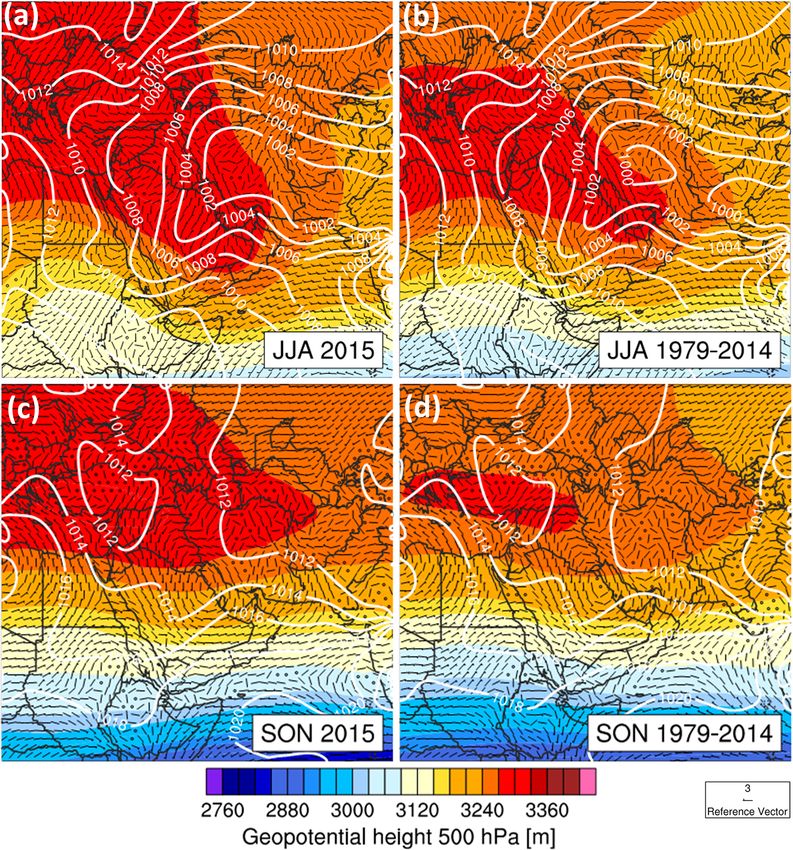
1616                                    O. Branch et al.: A comparison of the WRF model with 48 surface weather stations

   The model chain and configuration used in any simula-            data from 48 WMO-compliant surface weather stations dis-
tion can heavily influence the results of such forecasts. Im-       tributed over the UAE.
portant factors include but are not limited to the RCM type            Another objective is to assess the model performance in
(e.g., Coppola et al., 2020), general circulation model (GCM)       different areas of the UAE – which was split broadly into
dataset for boundary forcing (Gutowski et al., 2016; Jacob          three environments: (1) northern coastline and islands, (2) in-
et al., 2020), horizontal and vertical grid resolutions (e.g.,      land lowland desert areas, and (3) the Al Hajar Mountains
Schwitalla et al., 2017), physics and dynamics schemes (e.g.,       in the east. The aim is to investigate differences in perfor-
Chaouch et al., 2017; Schwitalla et al., 2020), and soil–land-      mance due to expected differences in climate regimes within
use–terrain static data, as well as internal model parameter        these zones, and their respective surface and landscape char-
sets for important land surface processes (e.g., Weston et al.,     acteristics and how they are dealt with by WRF with Noah-
2019).                                                              MP. Factors include, amongst others, the influence of sea
   The Weather Research and Forecasting (WRF) model                 surface temperatures in the warm and shallow Arabian Gulf
(Powers et al., 2017; Skamarock et al., 2008) has been used in      (Al Azhar et al., 2016), representation of albedo (Fonseca et
arid regions for various forecasting and verification purposes      al., 2020) and roughness length parameters (Weston et al.,
(e.g., Branch et al., 2014; Fonseca et al., 2020; Schwitalla        2019), and limitations in simulations over orography, partic-
et al., 2020; Valappil et al., 2020; Wehbe et al., 2019) and        ularly with respect to the wind field (e.g., Warrach-Sagi et al.,
process studies (Becker et al., 2013; Branch and Wulfmeyer,         2013). The Al Hajar Mountains have a complex climate with
2019; Karagulian et al., 2019; Nelli et al., 2020a; Wulfmeyer       regular coastal fog and convective events (e.g., Branch et al.,
et al., 2014). Currently, there have been few annual-scale          2020a). Therefore, splitting verification into the above zones
verification studies employing the WRF model on a NWP               (in which the stations are quite evenly distributed, with 17,
daily forecasting mode at such high spatiotemporal resolu-          15, and 16 stations, respectively) can yield further insights
tion (e.g., dx < 2–3 km). Horizontal grid scale is significant      into model performance and climate characteristics in differ-
because simulations employing convection-permitting (CP)            ent environments.
grid spacing (dx ∼ < 4 km) are known to outperform those at            Through ambitious simulations and robust verification,
coarser resolutions, particularly in terms of clouds and pre-       we can gain valuable insights into the regional climate and
cipitation – not least because they do not require a convection     model performance and take a step towards more skilful
parameterization (Bauer et al., 2015, 2011; Prein et al., 2015;     weather forecasting with WRF with Noah-MP in the UAE.
Schwitalla et al., 2011, 2017; Sørland et al., 2018). Further-         The structure of this work is as follows: we start with
more, it is known that land use, soil texture, and terrain inter-   our materials and methods (Sect. 2), showing maps of the
act with planetary boundary layer (PBL) processes in com-           study area and model domain (Sect. 2.1); a description of
plex feedbacks (e.g., Anthes, 1984; Mahmood et al., 2014;           the regional climate (Sect. 2.2); the model chain, configura-
Pielkel and Avissar, 1990; Smith et al., 2014) with a strong        tion, and simulation method (Sect. 2.3); verification dataset
level of land–atmosphere (LA) coupling thought to exist in          (Sect. 2.4); and verification methods (Sect. 2.5). Then fol-
this region (Koster et al., 2006). Representation of landscape      lows a results and discussion section (Sect. 3) and finally a
structure and the associated LA feedbacks should therefore          summary and outlook (Sect. 4).
be significantly improved when using finer grid resolution. In
terms of timescale, seasonal-to-annual simulations are costly
but provide a sufficient time series for robust statistical com-    2     Materials and methods
parison with observations over different seasons.
                                                                    2.1    Study area and model domain
   This study employs a configuration of WRF, coupled with
the NOAH-MP “multi-physics” land surface model (LSM),               The region under investigation is the United Arab Emirates
with modular parameterization options (Niu et al., 2011). In        (UAE) located between 22.61–26.43◦ N and 51.54–56.55◦ E
contrast to typical climate mode simulations, WRF is run            in the far northeast of the Arabian Peninsula (see Fig. 1a),
here in a numerical weather prediction (NWP), or daily fore-        with the 48 surface verification stations being spread out
casting, mode in order to keep conditions inside the domain         across the country. The model domain is shown in Fig. 1b
closer to that of the forcing data (see Sect. 2.3.3, for fur-       and covers a much larger area, (a) to be sure of excluding
ther details). We also apply high-quality and high-resolution       the area with the strong effects of the boundary forcing (i.e.,
boundary forcing data, improved static data for land use,           relaxation zone) from the analysis, and (b) to incorporate the
soils, terrain, high-frequency aerosol optical depth, and sea       large-scale synoptic weather situation. The model uses a reg-
surface temperature. This WRF configuration was employed            ular latitude–longitude grid and has corner grid cells located
and verified by Schwitalla et al. (2020) within a one-day case      at 14.775◦ N, 32.225◦ N, 43.275◦ E, and 65.725◦ E.
study of a physics ensemble.
   Our main objective is to assess the seasonal and diurnal
performance of WRF – both qualitatively and quantitatively
– in reproducing surface air temperature, dew point, and wind

Geosci. Model Dev., 14, 1615–1637, 2021                                              https://doi.org/10.5194/gmd-14-1615-2021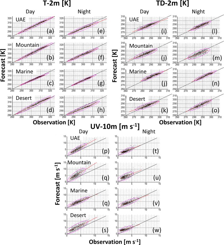
O. Branch et al.: A comparison of the WRF model with 48 surface weather stations                                                           1617

Figure 1. Panel (a) is a close-up of the study area overlaid with classified topography and 48 UAE surface weather stations used for
verification of WRF. Weather data were provided by the National Centre for Meteorology (NCM) in the UAE. The weather stations were
grouped into geophysical regions for statistical analysis. The 17 blue dots indicate coastal and marine stations (criteria – on islands or within
5 km from coastline). The 16 grey dots are mountain stations (criteria – any station ≥ 200 m a.s.l. and > 5 km from coast). The 15 orange dots
are inland desert stations (criteria – all remaining stations). Panel (b) is the 900 × 700 grid cell model domain (1x2.7 km, 2430 × 1890 km).
The four corner model grid cells are located at 14.775◦ N, 32.225◦ N, 43.275◦ E, and 65.725◦ E.

2.2     Regional climate                                                   cipitation is between 20 mm in the drier west to 130 mm in
                                                                           the higher Al Hajar Mountains of the east, mainly produced
2.2.1    Synoptic climate                                                  in the winter–spring time period (Sherif et al., 2014). During
                                                                           summer, subtropical subsidence leads to a strong reduction
Weather in the wider region is generally controlled by four                of precipitation and higher temperatures, and consequently
predominant patterns, including troughs originating from the               summer precipitation represents only around 20 % of the an-
Atlantic and Mediterranean Sea in winter, locally forced con-              nual amounts. However, upper-level disturbances from the
vective storms over the UAE and Oman Al Hajar Moun-                        southern monsoon flows can still transport moisture towards
tains in summer, and the southerly summer monsoon and cy-                  the Arabian Peninsula and the UAE (Böer, 1997; Schwitalla
clones from the Arabian Sea during June and October (Bru-                  et al., 2020), and convection is initiated sporadically over the
intjes and Yates, 2003; Steinhoff et al., 2018). These phe-                mountains of Oman and the UAE in summertime (Branch et
nomena are represented in large-scale seasonal climatolo-                  al., 2020a).
gies (1979–2014 – 08:00 UTC) in Figs. 2 and 3 (right-hand                     The neighboring Arabian Gulf to the north of the UAE
panels). To represent the climate, we have used geopotential               also plays a strong role in regional weather conditions. The
height at 500 hPa, wind velocity at 850 hPa, and mean sea                  prevailing winds from the Arabian Gulf are westerly or
level pressure. Note that winter is represented exclusively                northwesterly between January and May, but these change
by the months of January and February, because these are                   to northwesterly and then northerly directions from June to
the months used for our winter analysis during 2015 – for                  November. In the Arabian Gulf, which is relatively shal-
reasons of temporal continuity. In the climatology, we can                 low (maximum depth ∼ 90 m), particularly close to the UAE
clearly see a typical winter January–February (JF) low cen-                coast, the sea surface can heat rapidly, with temperatures of-
tered over Turkey and Iraq and a trough extending down to-                 ten exceeding 30 ◦ C (Al Azhar et al., 2016). Prevailing winds
ward the Arabian Peninsula. During summer, in June, July,                  are augmented by strong sea and land breezes, which develop
and August (JJA), we observe much higher temperatures fur-                 due to land–sea temperature gradients. Daytime sea breezes
ther south, with a heat low centered over Iran and the UAE.                can penetrate up to 50 km inland (Eager et al., 2008).
The other two seasons are transitional periods.
                                                                           2.3     Model chain and simulation method
2.2.2    UAE climate
                                                                           2.3.1    Model chain and physics
The UAE climate is generally characterized by scarce pre-
cipitation and high temperatures. However, annual cycles do                The model chain is based on the Weather Research and Fore-
exist with maxima of precipitation and minima of tempera-                  casting model version 3.8.1 using the Advanced Research
tures in winter and the converse in summer. Annual UAE pre-                WRF (ARW) core, which solves the Euler equations on a dis-

https://doi.org/10.5194/gmd-14-1615-2021                                                       Geosci. Model Dev., 14, 1615–1637, 2021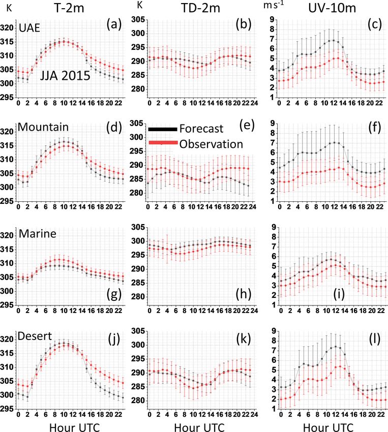
1618                                      O. Branch et al.: A comparison of the WRF model with 48 surface weather stations

Figure 2. Comparison of the 2015 (a) winter (January–February, JF) and (c) spring (March–May, MAM) large-scale fields at 08:00 UTC.
Panels (b) and (d) are an equivalent 36-year climatology between 1979 and 2014. Variables shown are geopotential height at 500 hPa (m;
shading), wind velocity at 850 hPa (m s−1 ; see reference vector at bottom right), and mean sea level pressure (hPa; white contours). Data are
taken from the ECMWF ERA5 reanalysis dataset.

cretized horizontal grid, with a terrain-following vertical co-          istan in the east. Care was taken, for reasons of model stabil-
ordinate system. The domain size and grid spacing matches                ity, that domain boundaries did not bisect very large peaks,
that of a previous simulation by Schwitalla et al. (2020) and            especially in the complex terrain of Iran. Vertically, 100 lev-
is comprised of a regular latitude–longitude grid with 900               els were used, adjusted so that at least 25 levels were present
by 700 cells horizontally (see Fig. 1b). In line with our pre-           in the lower 2000 m – to maximize resolution of the strong
vious statements on CP scale we selected a grid increment                moisture gradients in the boundary layer and lower tropo-
of 0.025◦ (dx ∼ 2779 m), with no parameterization of deep                sphere.
convection. It was important to extend the domain enough                    WRF was coupled with the NOAH-MP LSM (Niu, 2011)
to incorporate influential synoptic conditions upstream to the           to simulate land–surface processes and land–atmosphere
north, east, and southeast. Hence, our grid covers a region              feedbacks. NOAH-MP provides a separate vegetation canopy
of approximately 2500 km × 1945 km extending up to Iraq                  defined by a canopy top and ground layer including a modi-
in the north, down to the south of Yemen, and well into Pak-             fied energy balance closure approach. It offers a tile approach

Geosci. Model Dev., 14, 1615–1637, 2021                                                    https://doi.org/10.5194/gmd-14-1615-2021
O. Branch et al.: A comparison of the WRF model with 48 surface weather stations                                            1619

Figure 3. As for Fig. 2 but for summer and autumn: June–August (a, b) and September–November (c, d). Data were also taken from the
ECMWF ERA5 reanalysis dataset.

where the net longwave radiation and turbulent fluxes are cal-     aware component activated), the Mellor–Yamada 2.5 Level
culated separately for bare soil and the canopy layer. The         scheme (MYNN) for the atmospheric surface layer, and
calculated fluxes over vegetated grid cells are then bulked        the MYNN 2.5 level TKE scheme for the boundary layer
as a weighted sum of bare soil and canopy fluxes. Further-         (Nakanishi and Niino, 2006) (See Table 1 for a synopsis of
more, NOAH-MP is partially modular in structure, providing         physics schemes and their associated references).
a suite of optional schemes for several processes, such as ra-
diation budget calculation, stomatal resistance, snow albedo,      2.3.2   Initialization and forcing data
and others. The same configuration of Milovac et al. (2016)
was used for all NOAH-MP options.                                  Initial and lateral boundary conditions
   Other physics schemes included were the Rapid Radia-
tive Transfer Model (RRTMG) for long- and shortwave ra-            These were retrieved from the European Centre for Medium-
diation transfer (Iacono et al., 2008; Mlawer et al., 1997),       Range Weather Forecasts (ECMWF) Integrated Forecasting
the Thompson–Eidhammer microphysics scheme (Thomp-                 System (IFS), in the form of 6-hourly operational analysis
son and Eidhammer, 2014) (although without the aerosol-            data on the 41r1 cycle, on model levels. The horizontal grid
                                                                   increment is 0.125◦ (∼ 12 km) with 137 vertical levels up to

https://doi.org/10.5194/gmd-14-1615-2021                                             Geosci. Model Dev., 14, 1615–1637, 2021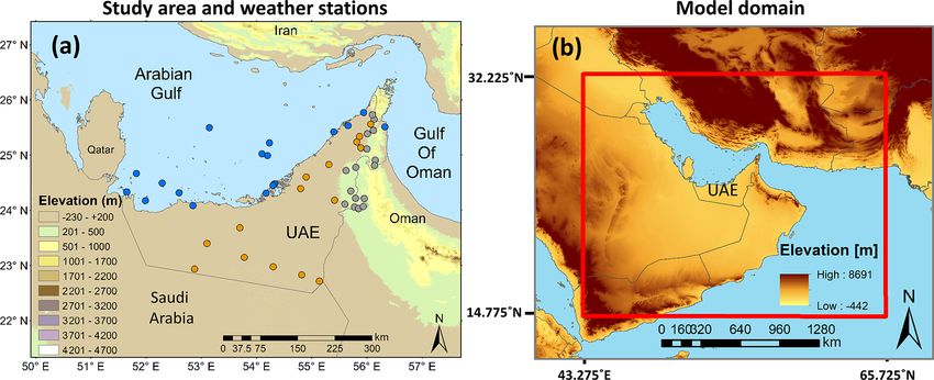
1620                                   O. Branch et al.: A comparison of the WRF model with 48 surface weather stations

Table 1. Selected physics schemes in WRF for sub-grid processes.

                      Physics type                   Scheme/option           Reference
                      Land surface scheme            NOAH-MP                 Niu et al. (2011)
                      Atmospheric surface layer      MYNN                    Nakanishi and Niino (2006)
                      Atmospheric boundary layer     MYNN 2.5 level TKE      Nakanishi and Niino (2006)
                      SW radiation                   RRTMG                   Mlawer et al. (1997)
                      LW radiation                   RRTMG                   Iacono et al. (2008)
                      Microphysics                   Thompson–Eidhammer      Thompson and Eidhammer (2014)

0.01 hPa. Soil moisture and soil temperatures are also pro-          were first reclassified in a logical manner before overwriting
vided by this model, which assimilates satellite soil moisture       the MODIS dataset within the UAE (see Schwitalla et al.,
data (Albergel et al., 2012) into its coupled Hydrology-Tiled        2020 for further details of this process).
ECMWF Scheme for Surface Exchange over Land (HTES-
SEL) model (Balsamo et al., 2009).                                   Terrain data

Sea surface temperatures (SSTs)                                      Here, we used the Global Multi-resolution Terrain Elevation
                                                                     Data (GMTED) 2010 static dataset (Danielson and Gesch,
These data were retrieved from the OSTIA project (Donlon             2011)
et al., 2012) – the data have a 1/20◦ horizontal grid spacing
at a 12-hourly frequency at 00:00 and 12:00 UTC. These data          2.3.3   Simulation method
are particularly important in coastal regions like the UAE.
                                                                     The objective of this study was to run a series of daily fore-
Aerosol optical depth (AOD) data                                     casts with WRF for the period 1 January to 30 Novem-
                                                                     ber 2015, with a discarded 1-month spin-up run from 1 De-
These data were retrieved from the ECMWF Monitoring At-              cember 2014. Note that December 2014 was not used for ver-
mospheric Composition and Climate (MACC) reanalysis (In-             ification (observation data were in any case not available at
ness et al., 2013), which interacts with the shortwave radia-        that time; see Sect. 2.4). It also makes sense not to analyze a
tion scheme to modify radiative transfer and diabatic heating        winter season split over 2 years.
– data have a ∼ 80 km horizontal grid spacing and a 6-hourly            The intention of carrying out such a long sequence was
frequency starting from 00:00 UTC.                                   to produce a long enough dataset to provide sufficient data
                                                                     points for robust statistical analysis. Forecasts were carried
Soil texture data
                                                                     out in NWP mode, i.e., with daily cold starts – as opposed
These data are an update from the default Food and Agri-             to a “climate” mode, which has a single cold start at the
culture Organization (FAO) dataset. The new data are based           outset. In NWP mode, a cold start was initiated each day
on the Harmonized World Soil Database (HWSD) v 1.2 at                at 18:00 UTC (22:00 LT) and run for 30 h, i.e., 6+24 until
30 arcsec grid spacing, where all the mapping units are re-          00:00 UTC the next day. The first 6 h of each forecast (18:00
classified into 12 soil and 4 non-soil types following the           to 00:00 UTC) were then discarded from the analysis. The
United States Department of Agriculture (USDA) soil clas-            6 h allows time for the atmosphere to spin up after each cold
sification system, as in the WRF model. For access to the            start – in particular for the residual boundary layer to develop
data and more details see Milovac et al. (2018). The WRF             and dissipate before the convective boundary layer starts to
default soil texture map based on the FAO data was used for          develop after sunrise (∼ 06:00 LT), and for potential cloud
the bottom soil layer.                                               development. Other UAE forecasting studies have also sug-
                                                                     gested that 5–6 h is an appropriate period for model conver-
Land use data                                                        gence in the UAE region (Chaouch et al., 2017; Weston et
                                                                     al., 2019). After discarding the first 6 h, a forecast remains
These data were provided as a combination of a high-                 for analysis spanning the 24 h of each day between 00:00 and
resolution dataset for the Emirates of Abu Dhabi and                 23:00 UTC (04:00 to 02:00 LT). See Table 2 for a summary
Dubai, provided by the National Center for Meteorology               of the simulation method.
(NCM), and the International Geosphere-Biosphere Pro-                   By reinitializing the 3D state within the domain itself (as
gramme (IGBP) Moderate Resolution Infrared Spectrora-                opposed to simply inputting lateral boundary conditions), we
diometer (MODIS) 20-class land use dataset, included within          ensure the atmospheric state is closer to the forecast provided
the WRF package (Fig. 4). The Abu Dhabi dataset contained            by ECMWF than would be the case in typical climate mode
some classes which differed from MODIS IGBP, and these               simulations. In climate mode, which is driven only at the

Geosci. Model Dev., 14, 1615–1637, 2021                                              https://doi.org/10.5194/gmd-14-1615-2021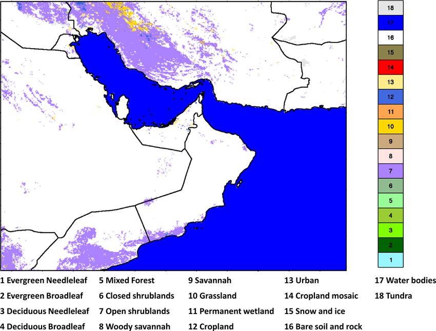
O. Branch et al.: A comparison of the WRF model with 48 surface weather stations                                                      1621

Figure 4. Map of whole model domain with the land cover dataset used in the simulation. It is a composite of the standard 30 arcsec (∼ 1 km)
IGBP 21-class MODIS dataset included as standard with WRF, with two local datasets superimposed: Abu Dhabi and Dubai Emirates,
obtained respectively from the Environment Agency of Abu Dhabi (EAD) and the International Center for Biosaline Agriculture (ICBA) in
Dubai. The local datasets were first reclassified in a logical manner into MODIS categories. 18 classes are shown here. There is a reduction
in resolution due to the grid increment of 2.7 km.

boundaries, the WRF simulations may diverge more strongly,              lateral boundary conditions are as for a climate mode run,
particularly toward the center of the large domain where the            i.e., input every 6 h from the forcing data. The atmospheric
study area lies, unless some form of interior nudging were              state within the domain boundaries is reinitialized each day
implemented (e.g., Lo et al., 2008).                                    at 18:00 UTC.
   An exception to the daily reinitialization of state variables
was made with the soil moisture field, whose state was in-              2.4    Datasets for verification
tentionally maintained from one successive day to the next,
by overwriting the soil moisture state from 18:00 to the next           Hourly verification data come from 48 surface weather sta-
day at 18:00, when the forecast is restarted. The intention             tions throughout the UAE (Fig. 1a and Appendix Table A1)
is to reduce physical inconsistencies between the soil mois-            and is quality checked and made available by the National
ture forecast in the driving GCM model and that of WRF                  Center for Meteorology (NCM) in Abu Dhabi, UAE. Fields
with Noah-MP. Intuitively that may not seem a large issue               available include air temperature at 2 m (T2 m ), dew point
given the aridity of the UAE. However, it becomes significant           at 2 m (TD2 m ) representing humidity, and wind speed at
when convective precipitation occurs in WRF, and soils are              10 m (UV10 m ). Data cover the entire period of 1 January–
wetted. Such convective events and flash floods are common              30 November 2015. Unfortunately, quality checked observa-
in the UAE and Oman, particularly from May to Septem-                   tion data for December 2014 were not available and so in
ber in the mountains, including during 2015 (Branch et al.,             the interest of preserving contiguous seasons, the month of
2020a; Schwitalla et al., 2020; Wehbe et al., 2019). Hence,             December 2015 was omitted from the winter statistics.
the NWP method is a worthwhile method of improving phys-
                                                                        2.5    Verification method
ical consistency. To summarize the NWP configuration: the
soil moisture is overwritten at 18:00 UTC from each consec-             An aim of the study is to assess WRF’s performance on sev-
utive day to the next, for the start of each new forecast. The          eral timescales: annually (January–November), seasonally,

https://doi.org/10.5194/gmd-14-1615-2021                                                    Geosci. Model Dev., 14, 1615–1637, 2021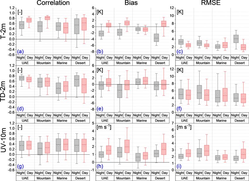
1622                                        O. Branch et al.: A comparison of the WRF model with 48 surface weather stations

Table 2. Summary of main aspects of simulation.

        Total duration of daily forecasts    1 December 2014 to 30 November 2015
        Period of analysis                   1 January to 30 November 2015
        WRF output frequency                 1-hourly
        Verification data frequency          1-hourly                                          48 surface weather stations
        Boundary forcing frequency           6-hourly                                          ECMWF operational analysis (0.12◦ )
        SST forcing frequency                6-hourly                                          OSTIA data
        AOD forcing frequency                6-hourly                                          ECMWF MACC reanalysis
        Land use data                        Static                                            MODIS IGBP – 21 classes
        Soil texture                         Static                                            Modified HWSD (Milovac et al., 2018)
        Terrain                              Static                                            GMTED 2010
        Cold start initialization            18:00 UTC daily
        Fields for reinitialization          All except soil moisture – all four soil levels
        Forecast length                      30 h (first 6 h discarded)
        Forecast analysis                    24 h – 00:00 to 23:00 UTC
        Model integration time step          15 s

daytime and nighttime periods, and hourly. Another aim is to               Regional analysis
assess performance within different regions of the UAE. The
exclusive assessment of overall forecast means over the UAE                We split the 48 UAE weather stations into three regions –
may be valuable but could obscure variability within the dif-              marine, mountain, and desert – based on surface geophysical
ferent regions, such as the capturing of high daytime tem-                 characteristics and proximity to water bodies (See Fig. 1a).
peratures in the inland deserts, or cooler and windier coastal             Accordingly, the following criteria were used for grouping
conditions.                                                                the weather stations into regions:
   Accordingly, the dataset was split temporally and spatially,
as follows.                                                                   – marine – located on islands or ≤ 5 km inland from the
                                                                                UAE coast (17 stations);
2.5.1   Temporal analysis
                                                                              – mountain – located in the Al Hajar Mountain area and
Yearly analysis                                                                 ≥ 200 m a.s.l. (16 stations);
                                                                              – desert – located > 5 km            distance   inland   and
Here, all time steps were analyzed from 1 January to
                                                                                < 200 m a.s.l. (15 stations).
30 November (hourly interval).
                                                                           The only exception made to this classification was for a sin-
Seasonal analysis
                                                                           gle station located at 204 m near the sand dunes of Liwa, in
                                                                           the south of the Abu Dhabi emirate. Although the station is
Here, we present the most extreme seasons in terms of air
                                                                           quite high, it is remote from the Al Hajar Range and was
temperatures – the (coolest) winter period of 1 January–
                                                                           deemed more suitable for a desert classification. Details on
28 February 2015 and the (warmest) summer period of 1 June
                                                                           altitude of the regional station groups can be found in Ta-
to 31 August 2015.
                                                                           ble 3, and a list of individual stations in the Appendix. The
Daytime and nighttime periods                                              desert region is characterized by barren or sparsely vegetated
                                                                           soils (as is most of the UAE), high surface temperatures,
For daylight hours we used all hours between 02:00 and                     and rapid nighttime cooling due to radiative losses associ-
13:00 UTC (06:00–17:00 LT) – and for nighttime, 14:00 to                   ated with a dry atmosphere. The Al Hajar mountain region
01:00 UTC (18:00–05:00 LT). These hours were selected                      is arid and has generally rocky bare slopes and lower albedo
based on the range of UAE sunrise and sunset which                         (e.g., Moody et al., 2005), with gravel plains running along
range between ∼ 05:30 and 07:00 and between ∼ 17:00 and                    the west side (Sherif et al., 2014).
18:50 LT respectively. The intention of separating day and                    One can assume some similarity between these regions,
night hours in this way is to examine performance during the               particularly when the synoptic situation is relatively homo-
nocturnal stable and daytime convective boundary layers. In-               geneous over scales larger than the study area. Nevertheless,
deed, several simulations in arid regions have demonstrated                given the large number of stations and length of time series,
nocturnal cold biases and an overestimation of daytime wind                if regional differences do exist then they should be evident.
speeds (Branch et al., 2014; Schwitalla et al., 2020; Weston
et al., 2019).

Geosci. Model Dev., 14, 1615–1637, 2021                                                        https://doi.org/10.5194/gmd-14-1615-2021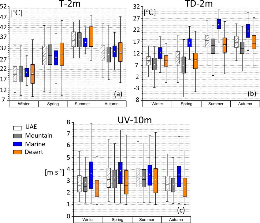
O. Branch et al.: A comparison of the WRF model with 48 surface weather stations 1623
Table 3. Number and altitude statistics for the regions – marine, The bias is a measure of overall error, including sign, defined
desert, and mountain. as follows:
ns
Region Number of Mean altitude Minimum Maximum 1 X
(fi − oi ) = f¯ − ō .
stations (m) (m) (m)
bias = (3)
ns i=1
Marine 17 13.8 0 101
Mountain 16 430.2 303 1485 These diagnostics were generated for 2015 for the region
Desert 15 120.0 114 204 and time period and their temporal distribution expressed
in boxplots (Sect. 3; Fig. 7) showing mean, median, 25 %–
75 % percentiles (box range), and 5 % and 95 % percentiles
2.5.2 Verification and diagnostics (whiskers).
Finally, a closer look at the diurnal evolution of the fore-
All comparisons were made using NCAR’s Model Evalua- cast is useful to investigate performance at specific times of
tion Tools V9.0 (MET) package (Brown et al., 2020), utiliz- day, such as local noon and at PBL transition periods, where
ing a nearest-grid cell approach on an hourly temporal reso- models often have biases. Hence, we generated mean hourly
lution. cycles of the spatial mean and spatial standard deviations for
To obtain a visual overview of model performance, in both forecast and observations. The mean at each hour is cal-
terms of closeness of fit, spread of forecast errors, and distri- culated as follows:
bution of residuals, scatterplots divided by region and day– T ns
night period are shown in Fig. 5. Included are a line of best 1X 1 X
mean(h) = oi or fi . (4)
fit for the data, a 1 : 1 line of perfect fit, and a 95 % confi- T t=1 ns i=1
dence ellipse. Then, we plotted regional seasonal statistics of
the mean observations (T2 m , TD2 m , and UV10 m ) (Fig. 6). The spatial standard deviation (σ ) at each hour is given as
To quantify the regional forecast–observation association, follows:
error magnitude, and sign during day and night, we show T u
v
ns
three standard statistical diagnostics: 1X u 1 X
σ (h) = t (oi − ō)2 or fi − f.¯ (5)
T t=1 ns − 1 i=1
– Pearson correlation coefficient
For the diurnal analysis, we selected the two most extreme
– root mean square error (RMSE) seasons in terms of temperature – the (coolest) winter period
of January–February (Fig. 8) and the (warmest) summer pe-
– bias. riod of June–August (Fig. 9) 2015. Again, these figures are
divided by region.
The Pearson correlation coefficient “r” measures the strength
of linear association between forecast (f ) and observation
(o), at all stations at each time step, given as follows: 3 Results and discussion
ns In this section, we present a discussion of the results. Be-
(fi − f¯)(oi − ō)
P
i=1
fore examining the model performance however, we first dis-
r=s s , (1) cuss the study period of 2015 in the context of the long-term
ns ns
P
(fi − f¯) 2
P
(oi − ō) 2 climate and El Niño (Sect. 3.1) to assess the representative-
i=1 i=1 ness of the 2015 study period. We then discuss differences
in regional climate and their significance to our verification
where fi and oi are the forecast and observation at each ob- (Sect. 3.2). Finally, we evaluate the regional model output of
servation point i, f¯, and ō are forecast and observation aver- T2 m , TD2 m , and UV10 m fields across the seasons and time
ages, ns indicates the total number of observations at each of day (Sect. 3.3).
time step (i.e., number of stations), and overbars indicate
the mean. Occasionally ns was reduced slightly whenever a 3.1 2015 in context
missing value occurred.
The RMSE is a scale-dependent diagnostic defined simply Our study period is from 1 January to 30 November 2015
as the square root of the mean square error (MSE) of the (during which time the full verification dataset was avail-
forecast: able). The year 2015 was considered one of the strongest El
Niño periods since 1950 (L’Heureux et al., 2017) with an
v
√
u
u1 X ns Oceanic Niño Index (ONI) index of up to 2.6 towards the
RMSE = MSE = t (fi − oi )2 . (2) end of the year (see Table 4). A high positive ONI indicates
ns i=1 a stronger El Niño event (a negative ONI indicates La Niña
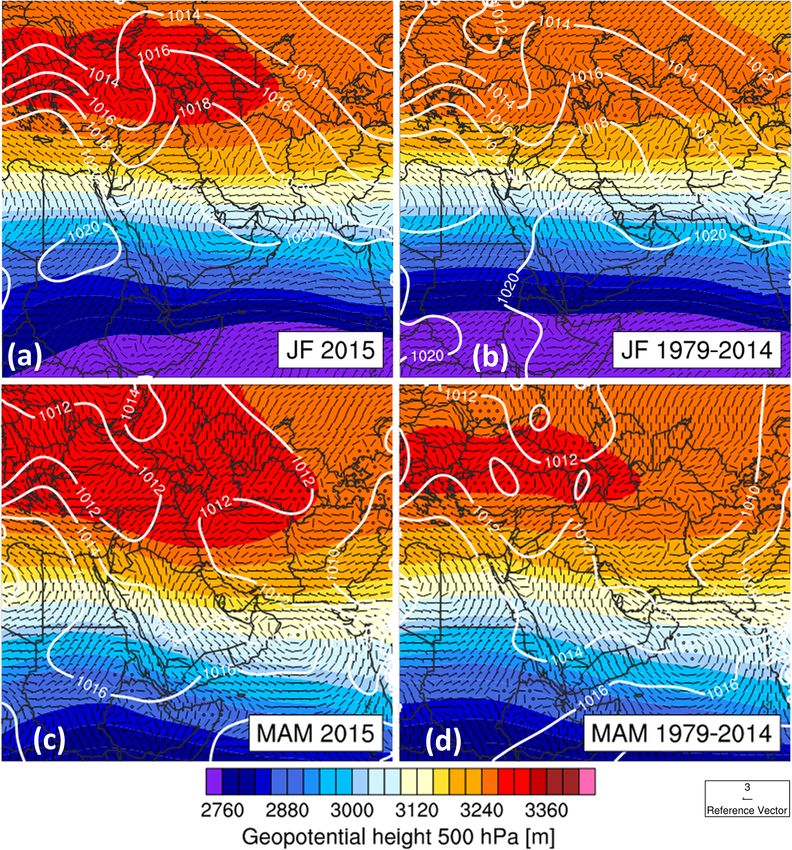
https://doi.org/10.5194/gmd-14-1615-2021 Geosci. Model Dev., 14, 1615–1637, 20211624 O. Branch et al.: A comparison of the WRF model with 48 surface weather stations Figure 5. Scatter plots of forecast vs. observation for all time steps over the period of January–November 2015, comparing each weather station at the corresponding WRF grid point. The plots are split by daytime (06:00–17:00 LT, left panels) and nighttime periods (18:00– 05:00 LT, right panels), and by region (UAE, mountain, marine, desert). The variables compared are 2 m air temperature (T2 m , K) in panels (a)–(h), 2 m dew point (TD2 m , K) in panels (i)–(o), and 10 m wind speed (UV10 m , m s−1 ) in panels (p)–(w). Also shown is a line of best fit (red), a line of perfect fit (black), and 95 % confidence ellipse (magenta). events). El Niño–Southern Oscillation (ENSO) is known to that a positive 2015 winter temperature anomaly exists to the impact upon the climate in this region, including tempera- north of the UAE, extending from Turkey to the Caspian tures and precipitation in the UAE (AlEbri et al., 2016; Al- Sea (Fig. 2, top left). However, conditions over the UAE mazroui, 2012; Chandran et al., 2016), so one might expect show less deviation in terms of the temperature, pressure, and significant climate anomalies during 2015. Hence, a com- wind fields. As the year progresses, and the ONI increases, parison was made between the long-term climatology and the temperature anomaly becomes more pronounced further the year 2015, based on ECMWF ERA5 reanalysis data. In south, especially in JJA when higher 2015 temperatures ex- Figs. 2 and 3, from the geopotential height field, we can see tend further south toward Oman and Yemen than is apparent Geosci. Model Dev., 14, 1615–1637, 2021 https://doi.org/10.5194/gmd-14-1615-2021
O. Branch et al.: A comparison of the WRF model with 48 surface weather stations                                                    1625

Figure 6. Regional seasonal statistics of mean observations: T2 m (a), TD2 m (b), and UV10 m (c). Box plots show the mean as a center line
and median as a dot; box ends are 25 % and 75 % percentiles, and whiskers are 5 % and 95 % percentiles.

in the climatology (Fig. 3a and b). Overall though, synop-             than the desert (∼ 1 ◦ C) in summer and autumn with the dif-
tic conditions over the Arabian Peninsula do not appear to             ference further reduced during spring and winter. The major-
be markedly different. They are similar enough, in fact, to            ity of mountain stations are located at fairly moderate alti-
consider the 2015 regional climate as representative of the            tudes (mean altitude 430 m; Table 3) with only one station
climate in general.                                                    located over 1000 m high (station ID 41229 – 1485 m a.s.l.;
                                                                       see Table A1 in Appendix). Even so, one might have ex-
3.2   Regional and seasonal characteristics                            pected larger differences. However, there could be reasons
                                                                       other than the temperature lapse rate for this, such as dif-
An assessment of regional distributions reveals that clear dif-        ferences in mountain and desert cloud cover (Branch et al.,
ferences in means and variability do exist (Fig. 6). As ex-            2020a; Yousef et al., 2019) or in albedo (e.g., Nelli et al.,
pected, the marine region is dominated by the Arabian Gulf             2020b).
characteristics, with more moderate temperature maxima and                TD2 m , or dew point temperature, is a standard measure of
minima (Fig. 6a), greater humidity (Fig. 6b), and higher wind          humidity and is in most cases relatively independent of the
speeds (Fig. 6c) than the inland desert (Fig. 6). Hence ma-            ambient temperature. It is also a reliable measure of how hu-
rine temperatures are lower than at the desert stations in the         mid the air feels in terms of human comfort (Wood, 1970).
summer months but remain higher in winter and autumn. In               In a hot (and warming) climate like the UAE, forecasting
fact, the desert stations have the most extreme T2 m range in          TD2 m accurately is therefore important for society. Region-
all seasons, reflecting the lower heat capacity surface, and           ally, we observe considerable differences in TD2 m (Fig. 6b),
consequent strong daytime surface heating. Rapid nocturnal             which are more or less expected due to coastal–land gradi-
cooling also occurs due to radiative losses in a much drier in-        ents and variation in vertical transport and distribution of va-
land environment. The mountain region is only a little cooler

https://doi.org/10.5194/gmd-14-1615-2021                                                   Geosci. Model Dev., 14, 1615–1637, 2021
1626 O. Branch et al.: A comparison of the WRF model with 48 surface weather stations
Figure 7. Box plots of T2 m , TD2 m , and UV10 m (respectively, panels a–c, d–f, and g–i) for all time steps over the period of January–
November 2015. Statistics are divided by region (UAE, mountain, marine, desert) and then by nighttime and daytime hours (respectively,
night 18:00–05:00 (grey boxes) and day 06:00–17:00 (red boxes) in local time). Statistics shown are Pearson correlation (a, d, g), bias (b, e,
h), and RMSE (c, f, i). On the box plots the center line represents the mean, the white circle is the median, box ends represent 25 % and 75 %
percentiles, and the whiskers are 5 % and 95 % percentiles. Also marked is a horizontal zero reference line for the Pearson and bias statistics.
Table 4. The 2015 Oceanic Niño Index (ONI) (3-month running mean of ERSST.v5 SST anomalies in the Niño 3.4 region at 50◦ N–50◦ S,
120–170◦ W), based on centered 30-year base periods updated every 5 years – NOAA.
Jan Feb Mar Apr May Jun Jul Aug Sep Oct Nov Dec
0.6 0.6 0.6 0.8 1 1.2 1.5 1.8 2.1 2.4 2.5 2.6
por in different environments. Table 5 shows the difference however, this contrast is reduced in the cooler seasons as the
in observed T2 m and TD2 m means. The inland atmosphere mountain and desert regions become more humid.
tends to be humid in summer when temperatures are high but There are significant regional differences in UV10 m , with
even closer to saturation in autumn and winter as tempera- marine UV10 m being 0.5–1 m s−1 higher than in other re-
tures fall, but humidity remains high. This seasonal range is gions (Fig. 6c) and also more variable. This is not unex-
particularly pronounced in the mountain regions, reflecting pected, due to low surface roughness, strong land–sea tem-
the predominance of annual rainfall occurring during win- perature gradients, and associated land–sea breezes. Desert
ter in the mountains and gravel plains of the northeastern UV10 m is the lowest all year round, and mountain UV10 m
part of the UAE (Sherif et al., 2014; Wehbe et al., 2019). falls in between those of the desert and marine regions. In
In all seasons, the marine region is closer to saturation than general, UV10 m is highest in spring and autumn.
in the other regions (T2 m minus TD2 m range is 8.3 to 11 ◦ C);
Geosci. Model Dev., 14, 1615–1637, 2021 https://doi.org/10.5194/gmd-14-1615-2021O. Branch et al.: A comparison of the WRF model with 48 surface weather stations 1627
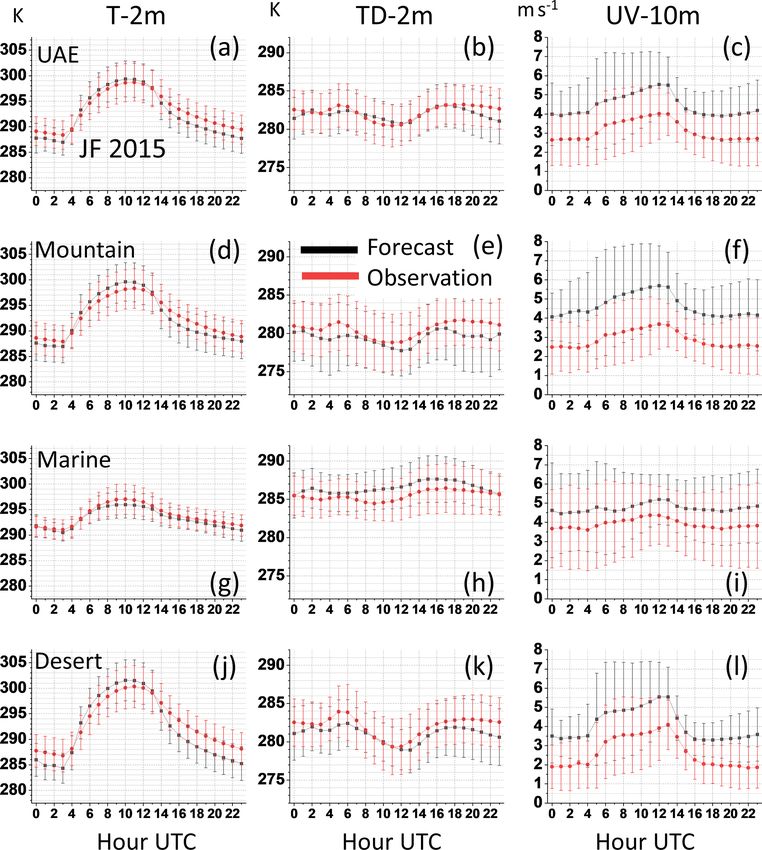
Figure 8. Winter diurnal cycles of spatial mean values of forecast (black lines) vs. observations (red) – January–February 2015. The error
bars represent the mean spatial standard deviation for each hour. Variables shown are T2 m (K, left panels), TD2 m (K, center), and UV-10
(m s−1 , right). Again the statistics are divided by region: UAE (top row), mountain (second row), marine (third row), desert (fourth row).
These regional differences justify the need for regional 3.3.1 T2 m
splitting of the dataset and are further addressed below, in
conjunction with model performance. In the scatter plots (Fig. 5a–h) we observe that in the day-
time, T2 m appears to be well estimated for the UAE on the
3.3 Model evaluation whole (Fig. 5a) (+0.44 ◦ C), and errors are well distributed
over the T2 m range. However, this agreement obscures some
Although the simulation of T2 m , TD2 m , and UV10 m and compensating regional biases; namely overestimation in the
causes for any biases may be physically linked, we never- desert (+0.71 ◦ C) and mountains (+1.06 ◦ C), and underesti-
theless first examine each field individually for clarity. mation in the marine region (−0.93 ◦ C).
Reasons for the warm bias may be attributable to a com-
bination of reasons. Firstly, a WRF overestimation of down-
https://doi.org/10.5194/gmd-14-1615-2021 Geosci. Model Dev., 14, 1615–1637, 20211628 O. Branch et al.: A comparison of the WRF model with 48 surface weather stations
Table 5. Seasonal and regional differences in observed T2 m and flected in all sub-regions, but not to the same degree. The best
TD2 m means to show the closeness to saturation. Included are the nocturnal performance is in the marine region (Fig. 5g) (bias
number of time steps for each season (NT ). Note that this is not a of −0.75 ◦ C), with an even error distribution across the tem-
mean of the differences between T2 m and TD2 m calculated at each perature range. The largest nocturnal cold bias is in the desert
time step, but an overall difference in means. region (−3.1 ◦ C) (Fig. 5h), with a steady increase in bias with
temperature. The switch from positive to cold biases usually
Season Region NT Mean (T2 m − TD2 m ) occurs more or less around the twice-daily transition times
total [◦ C]
of the boundary layer between stable and convective states.
Winter UAE 1416 11.2 Such arid nocturnal biases have been noted before (Branch et
Winter Mountain 1416 12.2 al., 2014; Fekih and Mohamed, 2017; Weston et al., 2019). It
Winter Marine 1416 8.3 may be that an overly dry lower atmosphere results in a lower
Winter Desert 1416 11.4 downward flux of longwave radiation, as found by Fonseca
Spring UAE 2207 18.6 et al. (2020) in a comparison of WRF with radiation mea-
Spring Mountain 2207 21.7
surements. All else being equal this dryness would lead to
Spring Marine 2207 11.0
Spring Desert 2207 20.4
a reduction of “buffering” at nighttime. They also found an
Summer UAE 2207 19.2 overly high upward ground heat flux during the night, which
Summer Mountain 2208 21.4 could be associated with sub-optimal soil parameters or an
Summer Marine 2208 10.5 overly strong soil–air temperature gradient. Overall, their net
Summer Desert 2207 22.0 radiation losses at night were higher in WRF than from the
Autumn UAE 2042 13.0 radiation measurements.
Autumn Mountain 2182 14.8
Autumn Marine 2176 8.9 3.3.2 TD2 m
Autumn Desert 2051 13.4
TD2 m is relatively well estimated in 2015 over the UAE as
a whole, with correlations around 0.7 and biases of less than
welling surface shortwave radiation has been observed be- 1 ◦ C (Fig. 7d and e, UAE sections). However, we can look
fore (Fonseca et al., 2020; Nelli et al., 2020b). This has been at regional and seasonal differences for more detail. In the
attributed to a lack of cloud cover but may also relate to the desert and marine regions, the biases are ≤ 1 ◦ C during both
performance of the radiative transfer scheme and interaction day and night. Marine TD2 m is slightly overestimated in gen-
with aerosols. Secondly, the soil representation, such as soil eral, indicating the model to be more humid over the gulf and
texture classification – and associated parameters like heat coast than observed. Mountain nocturnal dew points are more
capacity, thermal diffusivity, and albedo – may require ad- of a problem with a negative bias of ∼ −2 ◦ C, and a larger
justment. Underestimations of albedo in WRF have recently error spread than the other regions (Fig. 7e). There is also a
been observed, particularly for bright desert soils where mea- corresponding T2 m nocturnal bias of ∼ −2 ◦ C which could
surements show typical albedo values of 0.3 to 0.34 (Nelli et indicate a deficiency in the longwave surface budget as just
al., 2020b). The WRF albedo value in this study is around mentioned, but also a model deficiency in representing the
0.23 for much of the UAE lowlands, which would likely re- intermittent shear-driven turbulence that appears in nighttime
sult in an overly high net radiation and sensible heating, es- stable boundary layers. However, such biases in complex ter-
pecially on dry soils. This is consistent with the reported pos- rain have been already well documented (e.g., Warrach-Sagi
itive daytime temperature biases in the inland desert. A third et al., 2013; Zhang et al., 2013). One of the reasons cited
factor may be the prescribed aerodynamic roughness length is that the CP scale is not fine enough to resolve mountain
parameters used by WRF. Nelli et al. (2020a) found that a slopes and therefore cannot capture certain processes in the
new value for the parameter, derived from eddy covariance same way that large-eddy scale models can, with grid spac-
measurements, reduced the warm daytime bias in WRF sim- ings on the order of 1x = 100 m. However, while such fine
ulations (Nelli et al., 2020b). These causes may account for resolutions may be appropriate in a research context, they
some or all of the daytime temperature biases and therefore may remain prohibitively expensive and inappropriate in the
need to be considered for future simulations in this region. context of operational forecasting.
Nocturnally, we observe a cold bias over the UAE An additional problem in complex terrain is the validity
(Fig. 5e). This is quantified in Fig. 7b as a mean negative bias of the traditional Monin–Obukhov similarity theory (MOST)
of just over −2 ◦ C. One can also see that this nocturnal bias (e.g., see Foken, 2006) that is typically used in atmospheric
tends to worsen with an increase in daily T2 m , which implies models, including WRF, for calculation of model diagnos-
that the cold bias gets worse in the hotter months. This is con- tics like T2 m or TD2 m . MOST assumes homogeneous under-
firmed in the seasonal diurnal cycles (Figs. 8a and 9a), where lying land surface and stationary fluxes, and there is plenty
the mean nocturnal bias in winter is ∼ −2 ◦ C but increases to of evidence that in complex and heterogeneous landscapes
greater than −4 ◦ C in summer. This nocturnal cold bias is re- MOST needs significant improvements in scaling of turbu-
Geosci. Model Dev., 14, 1615–1637, 2021 https://doi.org/10.5194/gmd-14-1615-2021O. Branch et al.: A comparison of the WRF model with 48 surface weather stations 1629
lent kinetic energy profiles in the lowest part of the boundary different PBL schemes had little effect on positive UV bias
layer (e.g., Figueroa-Espinoza et al., 2014; Wulfmeyer et al., (Shimada et al., 2011). One additional factor is that there are
2018). The latter may affect representation of the heat, mois- several parameters within the MYNN scheme itself, which
ture, and momentum transport from the land surface to the may benefit from retuning for arid regions like the UAE
atmosphere, and if misrepresented may lead to such high bi- (e.g., Yang et al., 2017). However, the total impact of the
ases in the surface layer model diagnostics. PBL scheme selection on reproduction of the T2 m , TD2 m ,
Seasonally, diurnal TD2 m is quite well reproduced in both and UV10 m diagnostics is not completely clear. This is be-
winter and summer (Figs. 8 and 9). The mountain nocturnal cause, depending on the land surface type, the calculations
negative bias becomes more significant in summer (Fig. 9e). of transfer coefficients/fluxes are made in Noah-MP, the PBL
In the desert, a positive bias occurs over midday starting scheme, or the surface layer scheme (SLS). In WRF, PBL
around 10:00 LT (Fig. 9k) showing an overestimation of wa- schemes are generally coupled to the SLS, and typically all
ter vapor in summer. This is likely to be too early in the day variables between the land surface and lowest model layer
for a sea-breeze-driven anomaly but may relate to simulated are diagnosed (e.g. T2 m , U -10m, V -10m). These calcula-
soil moisture being higher than reality. This was observed tions in the SLS are based on Monin–Obukhov similarity
in a study by Wehbe et al. (2019) that found a wet bias in theory and are represented in the model as hard-coded pa-
dry soils and a dry bias in wetter soils in WRF over the UAE rameters and/or formulations of similarity functions. The lat-
when not coupled with a more advanced hydrological model. ter are used to obtain dimensionless bulk transfer coefficients
which are used for calculating momentum, heat, and mois-
3.3.3 UV10 m ture fluxes, and for diagnosing near-surface quantities like
T2 m . These coefficients re-enter the LSM and are to calcu-
WRF overestimates UV10 m during the day and night, in all late the surface fluxes which then enter the PBL scheme, as
regions and seasons. Positive biases of 1–2 m s−1 are typi- the lower boundary condition. Therefore, bias in near-surface
cal over the whole year (seen in Fig. 7h). Mountain daytime variables is strongly related to the choice of LSM and SLS. In
biases are strongest at 2 m s−1 , followed by daytime desert this WRF configuration, the communication link between the
biases at 1.5 m s−1 . Marine biases are lowest with mean bi- SLS and NOAH-MP is broken, as NOAH-MP itself calcu-
ases of < 1 m s−1 . Notably, there is a trend where positive lates transfer coefficients and diagnostics over land surfaces,
biases increase with wind speed (Fig. 5p, q, s). There is a effectively bypassing the SLS (Nielson et al., 2013). The SLS
significant increase in bias during the daytime, and also in only becomes active over water surfaces. This means that
the summer, particularly in the mountain and desert regions when NOAH-MP is used, the LSM probably has a stronger
(Fig. 9f and i). In fact, the strongest wind biases occur in impact on the bias of near surface variables than the PBL and
the same situations when daytime T2 m is overestimated, par- SLS (e.g., Milovac et al., 2016).
ticularly in the mountain and desert regions (Figs. 7, 8, 9), Incorrect aerodynamic roughness length parameters, as
hinting at a relationship between the two. Indeed, it is likely mentioned previously, may also play a large role in determin-
that an overly strong sea breeze may account for this. Dur- ing UV10 m – this parameter is used within the surface layer
ing summer, the desert-marine T2 m daytime gradient is high- scheme. Nelli et al. (2020a) found positive wind speed bi-
est (∼ 5 ◦ C; see Fig. 9g and j, red curves) than in winter ases over the same region when wind speeds were < 4 m s−1
(∼ 3 ◦ C; see Fig. 8g and j), although the seasonal warmth bi- and negative biases for wind speeds which were > 6 m s−1
ases are similar (∼ 1.5–2 ◦ C). The higher gradient coincides within a WRF V3.8 simulation. We have a similar behav-
with a greater UV10 m bias in summer. Weston et al. (2019) ior at night in the marine and desert regions, as exhibited by
improved the duration and direction of UAE sea breezes by the positive-to-negative distribution of errors increasing with
tuning a thermal roughness length parameter in WRF. The wind speed. Nelli et al. (2020a) reduced these biases by re-
PBL and surface layer parameterization schemes could also tuning the roughness length parameter based on eddy covari-
be a cause of the bias. Schwitalla et al. (2020) found an over- ance measurements (Nelli et al., 2020b).
estimation of UV10 m in all members of a UAE physics en- Another possibility is the length of the forecast spin-up,
semble, with magnitudes of around 1.5 m s−1 . The bias was the required length of which may still be uncertain. We have
worse when using the MYNN 2.5 TKE PBL and MYNN sur- already mentioned that Chaouch et al. (2017) cited a 5 h spin-
face layer schemes, when compared with the Yonsei Univer- up as being sufficient, but Hahmann et al. (2015) posit that
sity (YSU) scheme (Hong et al., 2006) paired with the MM5 the necessary spin-up over land could be 12 h or even more
Jiménez surface layer scheme (Jiménez et al., 2012). (primarily for effective use of the PBL scheme). However,
Using a non-local PBL scheme like YSU tends to pro- such long spin-ups are likely to be (i) prohibitively expensive
duce a deeper and drier PBL with a stronger vertical mixing, and (ii) too time consuming for forecasting purposes.
in comparison to local schemes like MYNN (see Milovac
et al., 2016; Yang et al., 2017). This may lead to a reduc-
tion in wind speeds, heat, and moisture close to the surface.
However, another study found that switching between seven
https://doi.org/10.5194/gmd-14-1615-2021 Geosci. Model Dev., 14, 1615–1637, 20211630 O. Branch et al.: A comparison of the WRF model with 48 surface weather stations
Figure 9. Summer diurnal cycles. As for Fig. 8 except for the period June–August 2015.
4 Summary and outlook on model performance with respect to specific processes and
land surface types, and how they are simulated.
An analysis of model predictions has revealed that WRF
The aim of this study was to (i) assess the skill of WRF with with Noah-MP represents the mean T2 m field reasonably
Noah-MP in reproducing surface quantities over the UAE; well during the daytime, although with a tendency for slight
(ii) identify regional, seasonal, and diurnal differences in per- overestimation (≤ 1 ◦ C). The nocturnal T2 m is underesti-
formance; and (iii) estimate potential sources of model de- mated more strongly though (1–4 ◦ C), and with larger biases
ficiencies. We have demonstrated the value of splitting the during the hotter months, particularly in the desert and moun-
model evaluation temporally and spatially. While assessment tains, likely due to a combination of deficiencies. The ma-
of diagnostics for the whole UAE region remains useful, it rine region has the lowest T2 m biases, which is encouraging,
can obscure regional, diurnal, and seasonal differences, as and highlights the value of ingesting quality SST data, es-
well as compensating biases. These are all scientifically in- pecially in coastal regions. WRF shows a good performance
teresting factors. Importantly, they might reveal information
Geosci. Model Dev., 14, 1615–1637, 2021 https://doi.org/10.5194/gmd-14-1615-2021O. Branch et al.: A comparison of the WRF model with 48 surface weather stations 1631 regarding TD2 m in general, with mean biases being ≤ 1 ◦ C. Humidity over the marine region tends to be slightly over- estimated though, whilst nocturnal mountain TD2 m is un- derestimated (bias ∼ −2 ◦ C). UV10 m performance on land still needs be improved, with biases of 1–2 m s−1 . Further- more, performance for UV10 m tends to worsen during the hot months, particularly inland. UV10 m in the marine region is generally much better simulated than in the other regions (bias ≤ 1 m s−1 ). There is an apparent relationship between T2 m bias and UV10 m bias, and this could be due to deficien- cies in sea–land breeze simulation. TD2 m biases appear to be more independent. The only exception to this is during the night, when T2 m and TD2 m biases do appear linked. Ultimately, no model downscaling forecast (at scales eco- nomically viable for forecasting) can be expected to exhibit exceptional skill in all conditions. A general caveat when evaluating models is that one must factor in a certain level of error in station or gridded observational datasets themselves (e.g., as discussed by Prein and Gobiet, 2017). Nevertheless, assuming a high level of observational accuracy, we have dis- cussed several avenues for improvement in this application of WRF. For instance, we should continue to devise and in- gest new and improved datasets for land cover, terrain and soil texture, and albedo. In particular, within a vegetation- sparse region like the UAE, soil texture, moisture, and other parameters are likely to be of prime importance. Certainly, ingesting SST data appears to have been valuable, given the lower coastal biases in all variables. We have mentioned several very useful experiments car- ried out on parameters like aerodynamic and thermal rough- ness lengths (Nelli et al., 2020a; Weston et al., 2019), as well as process-based observational studies related to the surface energy balance and verification studies (Fonseca et al., 2020; Nelli et al., 2020b). Further experiments should now be co- ordinated in order to improve model predictions further. In terms of parameterization schemes, ensemble experiments (in the manner of Chaouch et al., 2017; Milovac et al., 2016; and Schwitalla et al., 2020) are still required to identify op- timal land surface–surface-layer–PBL–microphysics combi- nations for arid regions. Such studies can also address the tuneable parameters defined inside parameterization schemes similarly to those conducted by Quan et al. (2016) and Yang et al. (2017). The most relevant ones can then be measured during dedicated field campaigns and subsequently ingested in the model. Seasonal-scale studies such as these are vital for accurate assessment of WRF nowcasting performance and to identify model deficiencies and areas for improvement. By combin- ing seasonal verification with sensitivity tests, and process and observational studies, we will move towards improved forecasting systems for the UAE and other arid regions. https://doi.org/10.5194/gmd-14-1615-2021 Geosci. Model Dev., 14, 1615–1637, 2021
You can also read