Seasonal and inter-annual variability of water column properties along the Rottnest continental shelf, south-west Australia - Ocean Science
←
→
Page content transcription
If your browser does not render page correctly, please read the page content below
Ocean Sci., 15, 333–348, 2019
https://doi.org/10.5194/os-15-333-2019
© Author(s) 2019. This work is distributed under
the Creative Commons Attribution 4.0 License.

Seasonal and inter-annual variability of water column properties
along the Rottnest continental shelf, south-west Australia
Miaoju Chen1 , Charitha B. Pattiaratchi1 , Anas Ghadouani2 , and Christine Hanson1
1 Oceans   Graduate School & the UWA Oceans Institute, the University of Western Australia, Perth, 6009, Australia
2 School   of Engineering, the University of Western Australia, Perth, 6009, Australia

Correspondence: Miaoju Chen (miaoju.chen@research.uwa.edu.au)

Received: 6 October 2018 – Discussion started: 26 October 2018
Revised: 7 March 2019 – Accepted: 11 March 2019 – Published: 4 April 2019

Abstract. A multi-year ocean glider dataset, obtained along       related to the changes in physical forcing (wind forcing,
a representative cross-shelf transect along the Rottnest conti-   Leeuwin Current, and air–sea heat and moisture fluxes).
nental shelf, south-west Australia, was used to characterise
the seasonal and inter-annual variability of water column
properties (temperature, salinity, and chlorophyll fluores-
cence distribution). All three variables showed distinct sea-     1   Introduction
sonal and inter-annual variations that were related to local
and basin-scale ocean atmosphere processes. Controlling in-       Almost all life forms rely on primary production, directly or
fluences for the variability were attributed to forcing from      indirectly, to survive, and phytoplankton in the ocean per-
two spatial scales: (1) the local scale (due to Leeuwin Cur-      form most of the primary production (Field et al., 1998).
rent and dense shelf water cascades, DSWC) and (2) the            Among the phytoplankton pigments, chlorophyll a (denoted
basin scale (El Niño–Southern Oscillation, ENSO, events).         as chlorophyll in the following description) is an important
In spring and summer, inner-shelf waters were well mixed          biological indicator of phytoplankton biomass in the water
due to strong wind mixing, and deeper waters ( > 50 m)            column. Environmental variables – such as light availability
were vertically stratified in temperature that contributed to     (Sverdrup, 1953; Huisman and Weissing, 1994), water tem-
the presence of a subsurface chlorophyll maximum (SCM).           perature (Eppley, 1992; Hambright et al., 1994; Paerl and
On the inner shelf, chlorophyll fluorescence concentrations       Huisman, 2008), and salinity (Karsten et al., 1995) – affect
were highest in autumn and winter. DSWCs were also the            phytoplankton biomass variability. Seasonal cycles of phy-
main physical feature during autumn and winter. Chlorophyll       toplankton concentrations are identifiable signals of the an-
fluorescence concentration was higher closer to the seabed        nual growth activity in pelagic systems (Cebrián and Valiela,
than at the surface in spring, summer, and autumn. The            1999; Winder and Cloern, 2010). In many parts of the world
seasonal patterns coincided with changes in the wind field        a spring bloom – an increase in phytoplankton concentrations
(weaker winds in autumn) and air–sea fluxes (winter cooling       in response to seasonal changes in temperature and solar ra-
and summer evaporation). Inter-annual variation was associ-       diation – is common and is usually present for a few weeks
ated with ENSO events. Lower temperatures, higher salinity,       to months (Cushing, 1959; Pattiaratchi et al., 1989). Often
and higher chlorophyll fluorescence (> 1 mg m−3 ) were as-        a secondary peak in production develops in late summer or
sociated with the El Niño event in 2010. During the strong        autumn (Longhurst et al., 1995). These seasonal phytoplank-
La Niña event in 2011, temperatures increased and salin-          ton patterns have large inter-annual variability across differ-
ity and chlorophyll fluorescence decreased (< 1 mg m−3 ).         ent geographic regions (Cebrián and Valiela, 1999; Cloern
It is concluded that the observed seasonal and inter-annual       and Jassby, 2008; Garcia-Soto and Pingree, 2009). Satellite
variabilities in chlorophyll fluorescence concentrations were     and field-based measurements have shown that in the olig-
                                                                  otrophic waters off south-west Australia, the seasonal chloro-
                                                                  phyll cycle (a proxy for phytoplankton biomass) is different

Published by Copernicus Publications on behalf of the European Geosciences Union.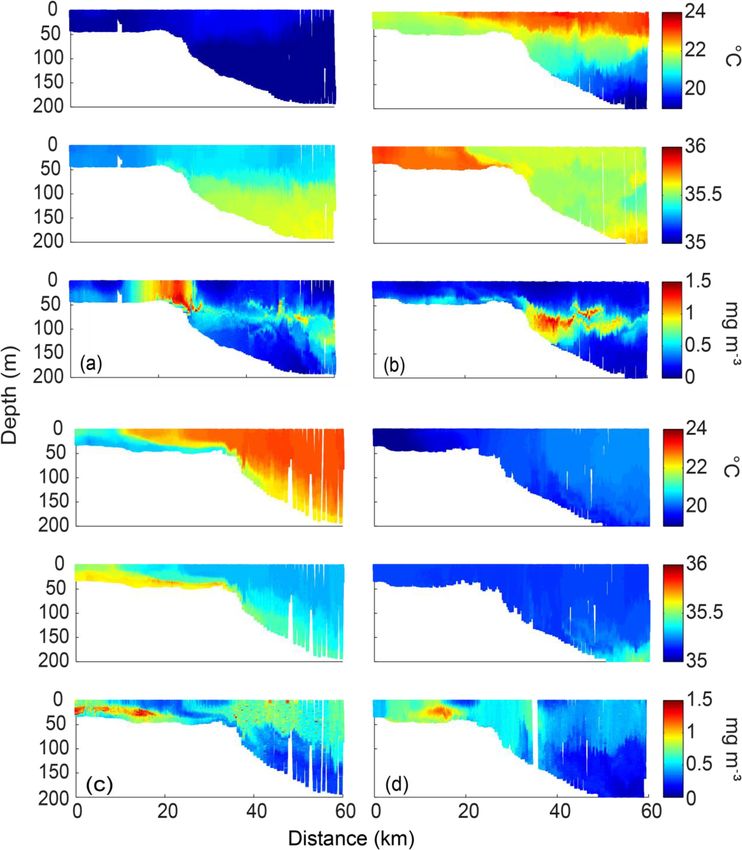
334        M. Chen et al.: Seasonal and inter-annual variability of water column properties (Rottnest continental shelf)

from that in other regions with a clear peak in chlorophyll        and offshore supply through eddy activity (Koslow et al.,
concentrations in late autumn or early winter and minimal          2008).
levels in spring and summer (Koslow et al., 2008; Thomp-              The RCS has several distinct bathymetric features
son et al., 2011; Lourey et al., 2012). Pearce et al. (2000)       (Fig. 1a): (1) a shallow inshore region (depths < 10 m),
found higher chlorophyll concentrations on the continental         which can be defined as a “leaky” coastal lagoon with a
shelf than further offshore. In this paper, we present an ex-      line of discontinuous submerged limestone reefs (Zaker et
tensive, multi-year, ocean glider dataset, obtained along a        al., 2007); (2) an upper continental shelf terrace with a grad-
representative cross-shelf transect along the Rottnest conti-      ual slope and a mean depth of ∼ 40 m, located ∼ 10–40 km
nental shelf (RCS), south-west Australia, to explore the sea-      from the coast; (3) an initial shelf break at the 50 m isobath;
sonal and inter-annual variability of water column properties      (3) a lower continental shelf between the 50 and 100 m iso-
(temperature, salinity, and chlorophyll fluorescence distribu-     baths, where the depth increases sharply; and (4) the main
tion). Although ocean gliders have been sampling the oceans        shelf break at the 200 m isobath.
for more than a decade, sustained observations addressing             The major current systems in the region are the Leeuwin
the variability at the seasonal and inter-annual timescales        and Capes currents (Woo and Pattiaratchi, 2008; Wijeratne
from continental shelf regions are almost non-existent and         et al., 2018). The LC is a warm lower-salinity poleward-
this study addresses this shortcoming.                             flowing eastern boundary current, which mainly flows along
   Changes in phytoplankton biomass at seasonal and inter-         the 200 m isobath (Ridgway and Condie, 2004; Pattiaratchi
annual timescales are important components of the total vari-      and Woo, 2009). In this oligotrophic environment lower
ability associated with biological and biogeochemical ocean        chlorophyll and nutrient concentrations (Hanson et al., 2005;
processes (Ghisolfi et al., 2015). The circulation along the       Twomey et al., 2007) and lower primary productivity (Han-
Western Australian coast has been studied through observa-         son et al., 2007; Koslow et al., 2008) characterise the LC.
tions and the use of ocean models (Gersbach et al., 1999;          The LC, which is strongest in autumn and winter, trans-
Feng et al., 2003; Twomey et al., 2007; Woo and Pattiaratchi,      ports ∼ 5–6 Sv (sverdrup) of water during austral winter and
2008; Wijeratne et al., 2018); however, methods to study           ∼ 2 Sv during austral summer poleward (Feng et al., 2003;
the biological processes in the water column have been lim-        Wijeratne et al., 2018). El Niño and La Niña cycles influence
ited to the use of satellite ocean colour data (Moore et al.,      the Leeuwin Current: the current is weaker during El Niño
2007; Lourey et al., 2012) and limited shipborne observa-          events and stronger during La Niña events (Pattiaratchi and
tions (Hanson et al., 2005; Pearce et al., 2006; Koslow et al.,    Buchan, 1991; Wijeratne et al., 2018). Of interest to this
2008). Satellite imagery is limited to processes at the sea sur-   study, the region experienced a marine heat wave in Febru-
face as sensors are unable to image subsurface waters due to       ary and March 2011, which was associated with the warming
limitations in light penetration. Information on the role of       related to the La Niña event defined as Ningaloo Niña (Feng
physical forcing and the biological responses in the water         et al., 2013). This event increased the Leeuwin Current’s vol-
column has been limited because of the absence of a com-           ume transport in February – an unusual event at this time of
prehensive observational dataset. In south-west Australia the      the year – and resulted in unprecedented warm sea surface
majority of the available oceanographic and biological data        temperature anomalies (∼ 5 ◦ C higher than normal) off Aus-
are restricted in time and space and are thus unsuitable to be     tralia’s west coast (Feng et al., 2013).
used to study seasonal and inter-annual patterns.                     The Capes Current, which is dominant in summer, is a
   Eastern boundaries of ocean basins are typically asso-          wind-driven inner-shelf current, generally formed in wa-
ciated with upwelling of nutrient-rich water into the eu-          ter depths < 50 m (Gersbach et al., 1999). It transports
photic zone leading to high primary productivity on the con-       cooler upwelling-derived water northward past Rottnest Is-
tinental shelf and rich coastal fisheries (Codispoti, 1983).       land (Fig. 1) between October and March (Pearce and Pat-
Oceanographic conditions off the RCS are dominated by the          tiaratchi, 1999; Gersbach et al., 1999).
Leeuwin Current (LC) that suppresses upwelling and trans-             Continental shelf processes along the Rottnest continen-
ports nutrient-poor water along the continental shelf and has      tal shelf are mainly wind driven, given the low diurnal tidal
a negative impact on primary productivity (Koslow et al.,          range (< 0.6 m; Pattiaratchi and Eliot, 2009). The seasonal
2008; Twomey et al., 2007). The absence of upwelling and           wind regime in the region can be divided into three regimes
major river systems means that the region is low in nutri-         (Verspecht and Pattiaratchi, 2010; Pattiaratchi et al., 2011):
ents. For example, Twomey et al. (2007) reported that dis-         (1) spring and summer (September–February) – strong daily
solved nitrate concentrations on the continental shelf and in      sea breezes dominate with southerly winds often exceeding
the surface 50 m further offshore were typically below de-         15 ms−1 ; (2) autumn (March–May) – the transition from the
tection levels (< 0.016 µM). Nitrate concentrations increased      summer to the winter regimes occurs, and wind speeds are
rapidly beyond 150 m depth to concentrations of around             usually low; and (3) winter (June–August) – storms occur
30 µM. Thus the RCS is a nutrient-poor environment with nu-        frequently. Storm systems are associated with the passage of
trient supply limited to that through recycling during storms      frontal systems with the region subject to peak wind speeds
                                                                   of 30 ms−1 . These winds are generally north-westerly in

Ocean Sci., 15, 333–348, 2019                                                                  www.ocean-sci.net/15/333/2019/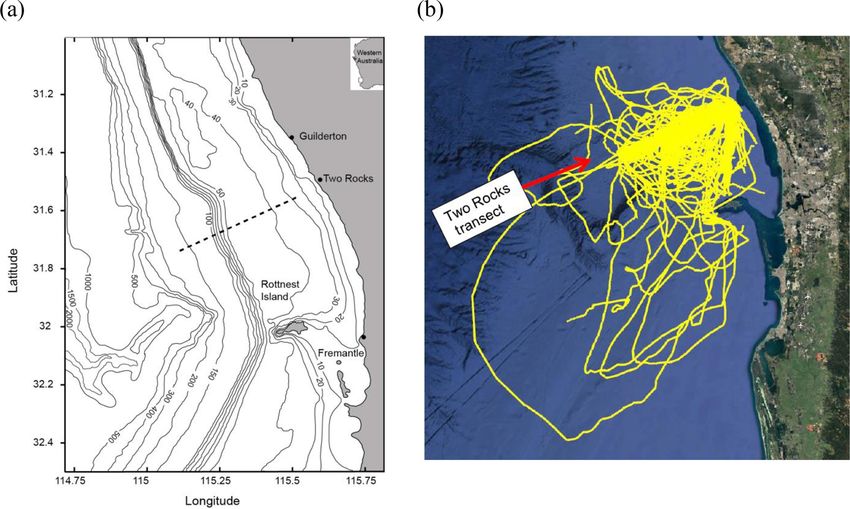
M. Chen et al.: Seasonal and inter-annual variability of water column properties (Rottnest continental shelf)                              335

Figure 1. (a) The study area. The dashed line denotes the location of the glider transect. Bathymetric contours are in metres; (b) tracks of all
the Slocum ocean glider deployments from 2009 to 2015.

winter and southerly in summer (Verspecht and Pattiaratchi,               salinity) gradient, DSWC is not present due to wind-induced
2010). In the study region winter storms have a typical pat-              vertical mixing.
tern with strong north and north-easterly components blow-                   The use of ocean gliders as an observational tool has sev-
ing for 12 to 52 h, followed by a period of similar duration              eral advantages over traditional ship-based surveys: ocean
when storms turn south and south-westerly with no prevail-                gliders have high sampling frequencies and long sampling
ing direction dominating for the duration of the storm. Sum-              durations (Pattiaratchi et al., 2017); the high temporal and
mer storms are southerly over a period of 3-4 days that are               spatial resolution data obtained with gliders may provide a
enhanced by the sea breeze system in the afternoon (Pat-                  better understanding of the links between the physical (mete-
tiaratchi et al., 1997; Gallop et al., 2012). Calm wind condi-            orological and oceanographic) forcing and the phytoplankton
tions are mainly observed during autumn and winter (March–                response; all the relevant data are collected simultaneously
August; between winter storm fronts) and are characterised                and are not weather limited. We used a multi-year (2009–
by low wind speeds (< 5 ms−1 ).                                           2015) ocean glider dataset (50 individual missions) along
   Another major feature of the dynamics is the presence of               a repeated transect to examine the variability in the phys-
dense shelf water cascade (DSWC) on the continental shelf                 ical parameters and chlorophyll fluorescence concentration
(Pattiaratchi et al., 2011). Western Australia experiences high           (a measure of phytoplankton biomass) distribution over sea-
evaporation rates resulting in higher salinity (density) water            sonal and inter-annual timescales. The 7-year timescale in-
in the majority of shallow coastal waters. This dense wa-                 cluded two El Niño events (2010 and 2014) and a strong ex-
ter is transported across the continental shelf close to the              tended La Niña event (2011–2013). The aims of this paper,
seabed due to the density difference between the nearshore                through the analysis of the long-term ocean glider dataset,
and offshore water (Pattiaratchi et al., 2011; Mahjabin et al.,           were to (1) examine the seasonal and inter-annual variabil-
2019). It is a major mechanism for the export of water con-               ity in chlorophyll fluorescence along the Rottnest continental
taining suspended material and chlorophyll away from the                  shelf; (2) relate the seasonal chlorophyll fluorescence vari-
coastal zone. Analysis of ocean glider measurements by Pat-               ability to changes in temperature and salinity distributions
tiaratchi et al. (2011) indicated that DSWC is a regular oc-              and local wind forcing; and (3) determine the influence of
currence along the RCS particularly during autumn and win-                the ENSO cycles on chlorophyll fluorescence. This is the first
ter months. In autumn the dense water formation is mainly                 long-term study of seasonal processes in the continental shelf
through changes in salinity resulting from evaporation whilst             waters along the RCS. This enables the identification of the
in winter, temperature was dominant through surface cool-                 main mechanisms that drive the variations in phytoplankton,
ing. In summer, although there is a cross-shelf density (due to           as represented by chlorophyll fluorescence along the RCS.

www.ocean-sci.net/15/333/2019/                                                                              Ocean Sci., 15, 333–348, 2019
336        M. Chen et al.: Seasonal and inter-annual variability of water column properties (Rottnest continental shelf)

  This paper is organised as follows. Sect. 2 describes the        CTD (conductivity–temperature–depth) sensor, a WETLabs
methods. The results of the seasonal winds and the monthly,        BBFL2SLO 3 parameter optical sensor (which measured
seasonal, and inter-annual variations in the chlorophyll and       chlorophyll fluorescence, coloured dissolved organic matter,
physical properties are described in Sect. 3. In Sect. 4 we dis-   and backscatter at 660 nm), and an Aanderaa oxygen optode.
cuss the possible causes of the observed variability. A general    All the sensors sampled at 4 Hz (which yielded measure-
conclusion is then given in Sect. 5.                               ments about every 7 cm in the vertical). The actual vehicle
                                                                   trajectory was transposed onto the Two Rocks transect as a
                                                                   straight line (Pattiaratchi et al., 2011).
2   Methods                                                           IMOS data streams are provided in NetCDF-4 format with
                                                                   ocean glider data files containing meta-data and scientific
Water column data were obtained from repeated sur-                 data for each glider mission. Subsequent to the ocean glider
veys undertaken using Teledyne Webb Research Slocum                recovery, all the data collected by the glider are subject to
electric gliders (http://www.webbresearch.com/, last access:       quality assurance and quality control (QA/QC) procedures
29 March 2019) along the Two Rocks transect off Rot-               that include a series of automated and manual tests (Woo,
tnest continental shelf, south-west Australia (Fig. 1). The        2017). To maintain data integrity, all of the sensors (CTD and
Slocum ocean glider is 1.8 m long, 0.213 m in diameter, and        optical sensors) are returned to the manufacturers for cali-
weighs 52 kg. It is designed to operate in coastal waters of       bration after a period 365 days in the water. The Sea-Bird
up to 200 m deep where high manoeuvrability is required            Scientific SBE 41CP pumped CTD sensor on the Slocum
under relatively strong background currents. Ocean gliders         gliders is the same as those mounted on Argo floats and
are autonomous underwater vehicles that propel themselves          achieve temperature and salinity accuracies of ±0.002 ◦ C
through the water by changing its buoyancy relative to the         and ±0.01 salinity units, respectively.
surrounding water (Rudnick, 2016). By alternately reduc-              The WETLabs BBFL2SLO 3 fluorescence values were
ing and expanding their ballast volume, ocean gliders can          estimated using the conversions provided by the manufac-
descend and ascend through the ocean water column using            turer. A recent study by Beck (2016) found that, through
minimal energy. In contrast to other similar automated ocean       inter-comparison between chlorophyll a derived from HPLC
sampling equipment (e.g. Argo floats; http://www.argo.ucsd.        (high performance liquid chromatography) and WETLabs
edu/, last access: 29 March 2019), ocean gliders have wings,       BBFL2SLO 3 fluorescence on ocean gliders, the original
a rudder, and a movable internal battery pack allowing them        manufacturer’s recommendation for the estimation of chloro-
to move horizontally in a selected direction in a sawtooth pat-    phyll a from fluorescence provided the best estimate. As
tern. This allows for the horizontal position to be controlled     part of the QA/QC procedures applied to the WETLabs
and to sample particular regions of the ocean. The gliders are     BBFL2SLO 3 Eco Puck sensor on the Slocum, gliders are
remotely controlled via the Iridium satellite system and nav-      subject to a series tests to track their performance, to iden-
igate through waypoints, fixing their position via the Global      tify errors, and to quantify drift during missions due to bio-
Positioning System (GPS). Each time the glider surfaces, the       fouling and/or damage. These tests were undertaken in the
data and new waypoints can be relayed via satellite to and         laboratory prior to shipping of the glider, immediately prior
from the glider. The autonomous nature of the ocean gliders        to deployment on the vessel, and then immediately on recov-
means that they are able to collect data continuously irrespec-    ery before cleaning of the sensor face. The tests were carried
tive of the weather conditions.                                    out by attaching a solid standard in a holder a set distance
   The dataset was collected over a 7-year period (2009–           from the sensor face and collecting engineering counts from
2015); gliders are operated by the Integrated Marine Observ-       the fluorescence, CDOM (coloured dissolved organic mat-
ing System (IMOS) ocean glider facility located at the Uni-        ter), and backscatter signals over a 5 min period. The solid
versity of Western Australia (Pattiaratchi et al., 2017). All      standards used for fluorescence and CDOM counts, Plexiglas
the ocean glider data are available through the Australian         Satinice® plum 4H01 DC (polymethylmethacrylate, Evonik
Ocean Data Network (https://portal.aodn.org.au, last access:       Industries), were identified by Earp et al. (2011) in a review
29 March 2019; AODN Portal., 2019). More than 200 cross-           of fluorescent standards for calibration of optical instruments
shelf transects from ∼ 50 ocean glider missions were anal-         as being the optimum. The ocean glider deployments started
ysed with ∼ 28 million individual scans obtained for each          in 2008 and performance of ECO Puck sensors has been doc-
variable (temperature, salinity, and chlorophyll).                 umented over this period. This included comparing consecu-
   Each cross-shelf ocean glider transect took 2 to 3 days         tive scale factors following factory calibrations. Our records
to complete (Pattiaratchi et al., 2011) with the gliders trav-     demonstrated the inherent stability of these sensors in their
elling at a mean speed of 25 km per day. The glider tran-          fluorescent and backscatter measurements with the differ-
sects extended from ∼ 20 m depth contour to deeper waters          ence between fluorescence scale factors between calibrations
(the gliders have a maximum depth range of 200 m) and col-         over 8 years of service typically < 6 %. To measure the re-
lected data from the surface to ∼ 2 m above the seabed. The        liability of the instruments between factory calibrations, the
gliders were equipped with a Sea-Bird Scientific pumped            fluorescent response of the instruments to a fluorescein con-

Ocean Sci., 15, 333–348, 2019                                                                  www.ocean-sci.net/15/333/2019/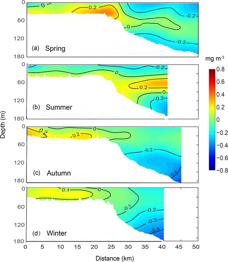
M. Chen et al.: Seasonal and inter-annual variability of water column properties (Rottnest continental shelf)                     337

Table 1. Mean values of temperature, salinity, and chlorophyll fluo-
rescence for each season used to calculate the cross-shelf anomalies.

                    Temperature     Salinity    Chlorophyll
                       (◦ C)                    fluorescence
                                                  (mg m−3 )
        Spring          19.4         35.35          0.49
        Summer          21.9         35.61          0.46
        Autumn          22.4         35.42          0.71
        Winter          19.8         35.27          0.68

centration curve has been tracked between factory calibra-
tions. We have also undertaken field measurements (Thom-
son et al., 2015) where a glider was attached to a rosette sam-
pler and collected concurrent data from the glider and Niskin
bottles at the surface, mid-depth, and bottom of the water col-
umn in 100 m depth. Water samples were subjected to HPLC
analyses to determine the “true” Chlorophyll a concentra-
tions. The comparison between WETLabs BBFL2SLO 3 de-
rived fluorescence and the HPLC chlorophylla concentra-
tions was very good with a correlation (r 2 ) value of 0.75
(n > 100) in the range 0.17 to 0.21 mg m−3 .
                                                                        Figure 2. Seasonal wind rose climatology for 2010–2014.
   Wind speed and direction, recorded at 30 min intervals,
were obtained from the Bureau of Meteorology weather sta-
tion at Rottnest Island, and located ∼ 40 km south of Two               3     Results
Rocks transect (Fig. 1a).
   The focus of this paper is on the seasonal and inter-annual          3.1    Seasonal winds
variability in the temperature, salinity, and chlorophyll flu-
orescence concentrations across the Two Rocks transect. It              The mean winds for each season from March 2010 to
was assumed that processes along this transect were rep-                March 2014 showed that southerly winds were prevalent in
resentative of the cross-shelf variability across the Rottnest          summer, autumn, and spring, followed by south and south-
continental shelf. When we refer to the “chlorophyll concen-            easterly winds (Fig. 2). Summer storms, which were usu-
tration” (units mg m−3 ), we are referring to the chlorophyll           ally associated with southerly winds, lasted up to 36 h with
fluorescence as recorded by the BBFL2SLO optical sensor.                speeds > 25 ms−1 . The sea breeze usually contributed to the
Salinity is expressed as a dimensionless quantity.                      southerly winds, which reinforced the prevailing southerly
   When examining the seasonal changes it was found that                winds found in the seasonal rose plots (Fig. 2). In autumn
the changes in the mean values obscured the seasonal vari-              the wind speeds decreased (< 13 ms−1 ), whereas in win-
ability of each parameter (temperature, salinity, and chloro-           ter the winds had no prevailing direction. This is typical
phyll). Hence, in addition to presenting the measured values            of winter storms, which are associated with rapid changes
(see Fig. S1 in the Supplement) we also calculated anomalies            in the wind direction (Verspecht and Pattiaratchi, 2010). In
to remove the influence of the seasonal variability. The pro-           spring, the winds were southerly with mean wind speeds of
cedure for each parameter (∼ 28 million individual points)              15 ms−1 . The southerly winds in the study region are up-
was as follows: (1) data were interpolated onto a common                welling favourable.
grid across the cross-shelf transect; (2) transects were then              The time series of the daily mean wind speeds and direc-
sorted according to season: spring (September–November),                tions in 2010 revealed the changes that occurred in the wind
summer (December–February), autumn (March–May), and                     regime: from November to May (the summer regime), the
winter (June–August); (3) the mean value across the whole               winds were generally southerly, and the mean wind speeds
transect (i.e. through water depth and across distance) for             were ∼ 7.5 ms−1 in November and ∼ 10 ms−1 in January
each season was calculated (Table 1); and (4) the anomaly               and February (Fig. 3). The wind speeds decreased between
at each grid point was calculated by subtracting the seasonal           March and mid-May (the autumn regime), with few changes
mean from values at each point.                                         in the wind direction. Between mid-May and October (the
                                                                        winter regime), winter storms caused large fluctuations in the
                                                                        wind speed and direction.

www.ocean-sci.net/15/333/2019/                                                                        Ocean Sci., 15, 333–348, 2019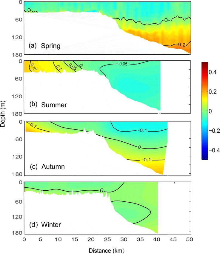
338         M. Chen et al.: Seasonal and inter-annual variability of water column properties (Rottnest continental shelf)

Figure 3. Time series of (a) mean daily wind speeds and (b) wind
direction in 2010 recorded at the Rottnest Island meteorological sta-
tion (Fig. 1).

3.2   Seasonal temperature, salinity, and chlorophyll
      distributions

Typical cross-shore distributions of the seasonal variation in
temperature, salinity, and chlorophyll along the Two Rocks
transect during spring, summer, autumn, and winter are
shown in Fig. 4.
   In spring (21–23 October 2013), the temperature and salin-
                                                                        Figure 4. Cross-shelf transects of temperature (◦ C), salinity, and
ity in the upper 80 m were vertically mixed across the whole
                                                                        chlorophyll (mg m−3 ) obtained along the Two Rocks transect
shelf. The temperature and salinity characteristics changed             in (a) spring (21–23 October 2013); (b) summer (28 February–
at the shelf break. On the upper continental shelf (< 40 m              3 March 2014); (c) autumn (18–21 May 2009); and (d) winter (9–
depth), the inshore waters were cooler and less saline than             11 August 2012).
the offshore waters (Fig. 4a). High chlorophyll concentra-
tions (up to 1.2 mg m−3 ) were found on the inner shelf and at
the 50 m shelf break (Fig. 4a), which corresponded to temper-
ature and salinity gradients (i.e. frontal system) in the same          tal shelf and depths > 180 m, was observed inshore and indi-
region. A thin layer (< 10 m) of subsurface chlorophyll max-            cated the presence of a DSWC. The maximum chlorophyll
imum (SCM, up to 1 mg m−3 ) extended from the shelf break               concentration (1.3 mg m−3 ) was located on the upper conti-
to offshore, and coincided with the halocline (and pycno-               nental shelf in the shallow pycnocline. The chlorophyll lev-
cline) at about 80 m depth.                                             els were generally higher in the DSWC than they were in the
   In summer (28 February–3 March 2014), a plume of warm                surface waters on the upper continental shelf. In the offshore
Leeuwin Current water (∼ 23.5 ◦ C) was located in the top               waters, higher chlorophyll water was uniformly distributed
∼ 30 m between 60 and 70 km offshore (Fig. 4b). This plume              in the surface mixed layer to depths of 60 m close to the shelf
cooled (to 23 ◦ C) and thinned (in the top ∼ 5 m) as it moved           break and depths > 120 m farther offshore (Fig. 4c).
inshore. Water on the upper continental shelf was cooler than              In winter (9–11 August 2012), the temperature increased
that offshore. The salinity on the upper continental shelf (∼           from 18 ◦ C inshore to 20.7 ◦ C offshore, and the water col-
35.7) was slightly higher than offshore (35.5); the Capes Cur-          umn was generally vertically mixed (Fig. 4d), except be-
rent most likely caused the cooler and saltier inshore waters.          tween 10 and 20 km on the upper continental shelf. The salin-
The cooler and saltier water on the upper continental shelf             ity was uniformly distributed inshore and in most offshore
revealed that higher-density water was present on the shelf             regions. Maximum chlorophyll (> 1 mg m−3 ) concentrations
and a small DSWC was present inshore of the shelf break.                were found along the inner shelf between 10 and 20 km and
A subsurface chlorophyll maximum (up to 1.2 mg m−3 ), be-               corresponded to the region of vertical and horizontal temper-
tween 50 and 110 m depths (at the pycnocline), was located              ature and salinity gradients.
from the shelf break to offshore.                                          The ocean glider data indicated vertical and horizontal
   In autumn (18–21 May 2009), the nearshore waters were                stratification across the shelf and the temperature and salin-
saltier and cooler (21 ◦ C) than the offshore waters (22.5 ◦ C)         ity distribution across the shelf changed seasonally. The tem-
(Fig. 4c). The offshore waters were well mixed except in the            perature and salinity characteristics on the upper continental
bottom 20 m. A plume of salty (35.7) and cooler (21 ◦ C) wa-            shelf were often different from those farther offshore. High
ter, which extended to ∼ 60 km across the entire continen-              chlorophyll concentrations were found in regions with strong

Ocean Sci., 15, 333–348, 2019                                                                        www.ocean-sci.net/15/333/2019/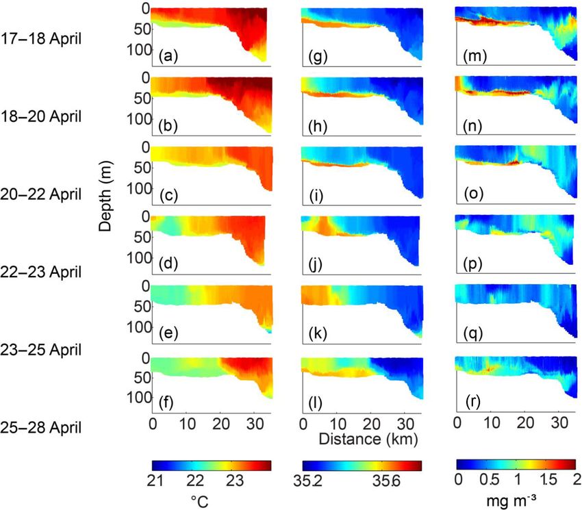
M. Chen et al.: Seasonal and inter-annual variability of water column properties (Rottnest continental shelf) 339
temperature and salinity gradients and thus density. These
maximum values occurred in the vertical (e.g. the SCM in
summer and autumn) and the horizontal (e.g. at the shelf
break in spring and winter).
3.3 Monthly mean temperature, salinity, and
chlorophyll concentrations
The monthly mean temperature and salinity for inshore and
offshore waters (upper 40 m depth) were calculated, except
during July, September, November, and December because
only a single ocean glider transect was available in each of
these months. The inshore waters were defined as the re-
gion where depth < 40 m, and offshore waters were defined
as the region where depth > 40 m. The temperature and salin-
ity structure indicated that from January to March (sum-
mer to early autumn), the inshore waters (< 40 m depth) in-
creased (∼ 21.1–23.0 ◦ C) and the salinity decreased (35.81
to 35.77) (Fig. 5a). From March to August (autumn to win-
ter), the temperature (23.0 to 19.0 ◦ C) and salinity (35.77
to 35.22) both decreased. From August to January (winter to
early summer), both temperature (18.9 to 21.1 ◦ C) and salin-
ity (35.22 to 35.8) increased. Offshore water (> 40 m depth)
showed a similar seasonal pattern to that of the inshore wa-
ters (Fig. 5b). Except that from January to March the salinity Figure 5. Monthly averaged temperature–salinity diagram with the
decrease in offshore waters (from 35.71 to 35.54) was larger chlorophyll (Chl) values (mg m−3 ) for the Two Rocks transect be-
compared to inshore waters, and from August to January the tween 2009 and 2015. The horizontal error bars indicate the stan-
offshore water temperature dropped slightly before increas- dard deviation of salinity, and the vertical error bars indicate the
ing to 21.0 ◦ C. standard deviation of temperature.
Spatially averaged chlorophyll concentrations for the
inshore waters revealed significant seasonal variability
(Fig. 5a). Higher chlorophyll concentration values were 3.4.1 Temperature anomaly
reached between March and August (autumn to winter)
with a maximum of 1.12 mg m−3 reached in May that
Seasonal temperature anomaly in the continental shelf wa-
decreased to a minimum of 0.36 mg m−3 in February.
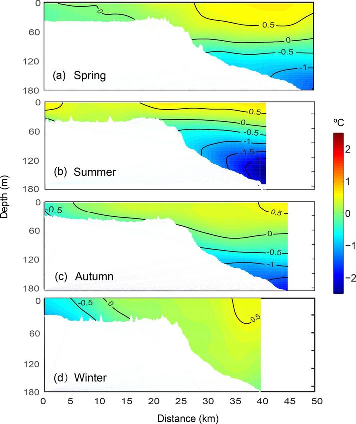
ters differed from those further offshore, seaward of the shelf
The chlorophyll concentration values for offshore waters
break (Fig. 6). During spring, the temperature distribution
were less variable with highest values in May (maximum
showed water to be vertically well mixed on the upper con-
of 0.85 mg m−3 ) and lowest in February (minimum of
tinental shelf (Figs. 6a and S1a) and vertically stratified in
0.43 mg m−3 , Fig. 5b). Higher chlorophyll concentrations
depths > 40 m. The offshore water in the upper layer was
corresponded with warmer and less-saline water for both the
warmer compared to water on the inner shelf. In summer, the
inshore and offshore waters.
warmer surface water extended across the entire continental
shelf (Fig. 6b). Water along the middle of the shelf (5–20 km
3.4 Seasonal distribution from the coast) was slightly cooler, most likely due to the
influence of the Capes Current. In autumn and winter, the
upper-shelf waters were cooler than the offshore waters. The
Over the 7-year study period (January 2009–March 2015), temperature anomalies were mostly negative with the low-
the vertical structure of the seasonal mean data for the Rot- est values (−1 ◦ C) attained close to the coast (between 0 and
tnest continental shelf revealed variability in temperature, 7 km) (Fig. 6c and d).
salinity, and chlorophyll concentrations. Anomalies are de- The largest variability in the offshore waters was asso-
fined as departures from the seasonal average with positive ciated with the thermocline depth (temperature anomaly of
(negative) values higher (lower) than the seasonal average. about −1.0 ◦ C). In spring, the thermocline was almost hori-
The anomalies allowed us to examine the relative changes in zontal and located at ∼ 120 m depth. In summer, the thermo-
water properties across the whole transect for each season. cline was located higher in the water column (∼ 70 m depth)
www.ocean-sci.net/15/333/2019/ Ocean Sci., 15, 333–348, 2019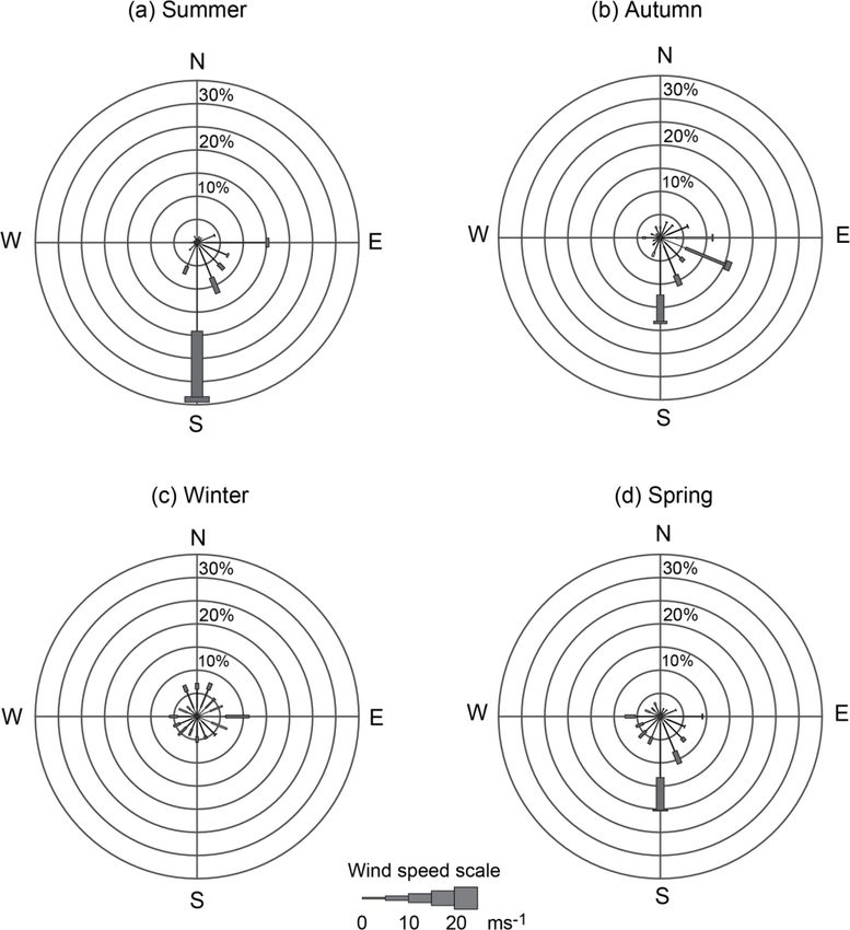
340         M. Chen et al.: Seasonal and inter-annual variability of water column properties (Rottnest continental shelf)

                                                                        Figure 7. Mean vertical structure anomaly of the salinity in
Figure 6. Mean vertical structure anomaly of the temperatures (◦ C)     (a) spring, (b) summer, (c) autumn, and (d) winter, averaged sea-
in (a) spring, (b) summer, (c) autumn, and (d) winter, averaged sea-    sonally over distance and depth across the Rottnest continental shelf
sonally over distance and depth across the Rottnest continental shelf   between 2009 and 2015.
between 2009 and 2015.

                                                                        (i.e. not at the surface) and along the upper shelf. In spring,
with a slight inclination (deeper in the offshore). In autumn,          the highest chlorophyll concentration anomaly was found
the thermocline depth increased to 100 m with a more pro-               at the shelf break (Fig. 8a) and was related to a horizontal
nounced inclination. The thermocline inclinations in sum-               temperature gradient (Fig. 6a). An SCM at ∼ 100 m depth
mer and autumn were most likely due to upwelling processes              was present in the offshore waters aligned with the vertical
when the winds were upwelling favourable (Fig. 2). In win-              stratification in temperature, salinity, and density (Figs. 6a,
ter, the thermocline was absent because the Leeuwin Current             7a, and S4b). In summer, the SCM was concentrated over
dominated the offshore waters.                                          a smaller depth range (< 50 m) in the offshore waters. On
                                                                        the continental slope, seaward of the shelf break (an area
3.4.2   Salinity anomaly                                                of 20–30 km), the chlorophyll concentration anomalies were
                                                                        more diffuse, most likely because of the variation in the up-
In summer and autumn, the salinity anomaly was higher on                welling and the diurnal cycle (Chen et al., 2017). In autumn
the upper shelf than in the offshore waters, mainly because             and winter, the SCM was absent, but the chlorophyll con-
of evaporation (Fig. 7b and c). A cross-shelf salinity gra-             centration anomalies were higher on the upper continental
dient was also present. The salinity was more uniform in                shelf. The autumn chlorophyll distribution corresponded to
the surface waters offshore. In spring, high salinity water             the presence of DSWCs on the upper shelf (Figs. 7c and 8c).
was present at > 100 m corresponding to the colder water
(Fig. 7a). In winter, salinity gradients were absent along the          3.5   Depth-integrated mean variability
whole transect (Fig. 7d).
                                                                        We used a 7-year dataset of ocean glider deployments to ex-
3.4.3   Chlorophyll concentration anomaly                               amine the inter-annual variability in the temperature, salin-
                                                                        ity, and chlorophyll concentrations. Water properties were
The chlorophyll concentration anomalies revealed there there            depth-averaged from the surface to 30 m depth (Fig. 9). The
were seasonal variations in the upper-shelf and offshore wa-            gliders traverse in a sawtooth pattern, and as the depth in-
ters (Fig. 8). Across the whole transect, high chlorophyll con-         creases the surfacing spacing increases; thus there were gaps
centration anomalies were present in the subsurface waters              in the data for the deeper waters. All the water properties

Ocean Sci., 15, 333–348, 2019                                                                         www.ocean-sci.net/15/333/2019/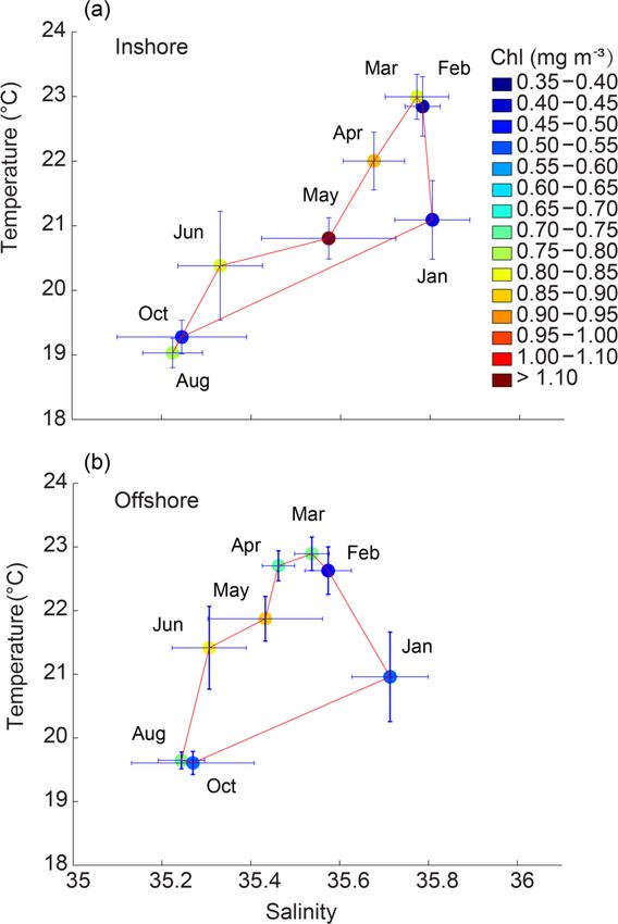
M. Chen et al.: Seasonal and inter-annual variability of water column properties (Rottnest continental shelf) 341
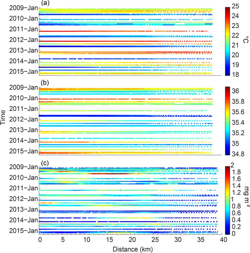
Figure 9. Time–distance series of the (a) temperature (◦ C),
(b) salinity, and (c) chlorophyll (mg m−3 ), averaged for the top 30 m
of water along the Rottnest continental shelf between January 2009
Figure 8. Mean vertical structure anomaly of the fluorescence and March 2015. Zero distance (0 km) denotes the start of the glider
(mg m−3 ) in (a) spring, (b) summer, (c) autumn, and (d) winter, av- transect.
eraged seasonally over distance and depth across the Rottnest con-
tinental shelf between 2009 and 2015.
showed seasonal changes, but in this section we focus on the
inter-annual variability. For example, the marine heat wave
during the 2011 La Niña events is evident (red lines - sum-
mer 2011) as well as the cooler summers in 2009 and 2015
(yellow lines). Similarly, higher salinities were recorded dur-
ing summers 2010, 2014, and 2015 that were associated with
El Niño events (red lines). Figure 10. Time series of the depth-averaged temperature, salinity,
The year-to-year summer temperature range was > 4 ◦ C: and chlorophyll 10 km from the start of the glider transects.
the temperature was < 20.1 ◦ C in February 2010 and in-
creased to a maximum of 24.4 ◦ C in March 2011 and also
in February 2012 (Fig. 9a). This maximum temperature was tions was from March 2011 (chlorophyll concentration of
associated with the persistent La Niña event in 2011–2012. 0.88 mg m−3 ) to March 2014 (chlorophyll concentration of
In winter, the year-to-year temperature range was > 3 ◦ C: the 0.14 mg m−3 ). The lowest value of 0.18 mg m−3 was also
temperature was > 21.2 ◦ C in 2011 and decreased to a mini- recorded in March 2013.
mum of 18.4 ◦ C in 2012 and 2014. Time series of the depth-averaged (surface 30 m) temper-
The concurrent depth-averaged salinity time series showed ature, salinity, and chlorophyll measured 10 km from the
that the waters were less saline (34.9) in August 2011 than coastline revealed strong seasonal and inter-annual variabil-
they were in other years (Fig. 9b). In March 2015, the high- ity, especially in response to El Niño and La Niña events
est salinity value (∼ 35.9) was measured on the upper shelf. (Fig. 10). Information presented in Fig. 10 includes the same
The lowest value (∼ 35.5) was attained in 2011 and was as- as that shown in Fig. 9, except that variations at a single
sociated with the warmer water. point (10 km) are shown as a time series. The seasonal cy-
The depth-averaged chlorophyll concentrations also had cle (Sect. 3.3; Fig. 5a) indicated warmer saltier water was
strong inter-annual variation (Fig. 9c) with values ranging present in summer and cooler less-saline water in winter.
from 0.81 mg m−3 in May 2009 and 2010 to 1.8 mg m−3 in In 2009/2010, a moderate El Niño event occurred, which
May 2014. The largest range in the chlorophyll concentra- resulted in lower temperatures and higher salinity during the
www.ocean-sci.net/15/333/2019/ Ocean Sci., 15, 333–348, 2019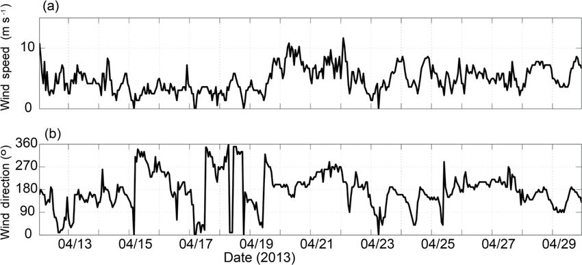
342        M. Chen et al.: Seasonal and inter-annual variability of water column properties (Rottnest continental shelf)

Figure 11. (a) Wind speed (ms−1 ) and (b) wind direction (◦ ) along
the Rottnest continental shelf between 12 and 30 April 2013.

first half of 2010. The El Niño weakened the Leeuwin Cur-
rent, which entrained cooler saltier water into the region from
offshore (e.g. Woo and Pattiaratchi, 2008). The chlorophyll
values were ∼ 1 mg m−3 , with a slight elevation in winter
due to the seasonal bloom (Fig. 10).
                                                                      Figure 12. Vertical cross-sections of (a–f) temperature (◦ C), (g–
   The 2009/2010 El Niño was followed by a strong ex-
                                                                      l) salinity, and (m–s) chlorophyll (mg m−3 ) across the Rottnest con-
tended La Niña between 2011 and 2014. The ocean glider                tinental shelf between 17 and 28 April 2013 obtained with the ocean
data (Fig. 10) captured several El Niño and La Niña ef-               glider.
fects in the water column properties. (1) A maximum tem-
perature (> 24 ◦ C) was recorded in February 2011, which
was an increase of > 4 ◦ C from 2010. From 2011 to 2014,
                                                                         The winds and the vertical stratification also affected the
summer temperatures decreased. (2) A significant drop in
                                                                      chlorophyll distribution. Initially, high chlorophyll concen-
salinity (> 0.5) occurred from 2010 to 2011. This salin-
                                                                      trations were found in the DSWC on the upper shelf close to
ity decrease was mainly due to a stronger Leeuwin Current
                                                                      the seabed and in the SCM in the offshore waters (Fig. 12m).
transporting lower-salinity water into the region. From 2011
                                                                      As the winds increased, the chlorophyll concentration be-
to 2014, the salinity increased. (3) Chlorophyll decreased
                                                                      came uniform through the water column across the whole
from ∼ 1 mg m−3 in 2011 to < 0.25 mg m−3 in early 2014
                                                                      transect (Fig. 12q). Note that the wind, although not strong
and then increased in May 2014.
                                                                      (∼ 10 ms−1 ), was able to mix the water column to ∼ 80 m
3.6   Temperature, salinity, and chlorophyll during a                 depth in the offshore waters and erode the thermocline and
      storm event                                                     thus the SCM. The SCM likely reformed (Fig. 12s); how-
                                                                      ever, with reduced solar heating and convective cooling, the
The ocean glider data obtained from 17 to 28 April 2013               stratification would have weakened, which would have led to
revealed that a storm caused vertical mixing in the wa-               a well-mixed water column in late autumn and early winter.
ter column and transported higher chlorophyll water from
the SCM to the surface. The first two transects (17–
20 April 2013) were collected under low wind (< 5 ms−1 )
conditions (Fig. 11). The water column was vertically strat-          4   Discussion
ified across the whole transect with a DSWC present on the
upper shelf (Fig. 12a and b). Higher chlorophyll water was            In this paper, simultaneous water column data of ocean prop-
present in the DSWC’s bottom layer. In the deeper waters,             erties (temperature, salinity, and chlorophyll fluorescence)
the higher chlorophyll water was associated with the SCM              together with meteorological data were used to examine the
(Fig. 12m and n).                                                     seasonal and inter-annual variability along the Rottnest con-
   On 20 April, the winds increased to > 10 ms−1 . The winds          tinental shelf. Acquisition of multi-year sustained ocean ob-
were initially southerly and then changed to westerly and             servations using shipborne sampling is difficult (relative high
continued to be that way until 23 April (Fig. 11) causing             cost and weather dependence) and thus many studies have
vertical mixing of the water column. By 25 April, the wa-             used satellite remote sensing data of sea surface temperature
ter column on the upper shelf was vertically mixed (Fig. 12e          and ocean colour to determine seasonal and inter-annual vari-
and k). On 28 April, when the winds decreased, the water              ability on continental shelves (e.g. Nieto and Mélin, 2017;
column on the upper shelf was vertically stratified in salinity       Kilpatrick et al., 2018). Here, ocean glider data collected
(Fig. 12l).                                                           along a single transect along the RCS shelf over the pe-
                                                                      riod 2009–2015 indicated distinct seasonal and inter-annual

Ocean Sci., 15, 333–348, 2019                                                                       www.ocean-sci.net/15/333/2019/
M. Chen et al.: Seasonal and inter-annual variability of water column properties (Rottnest continental shelf) 343 variation in temperature, salinity, and chlorophyll concentra- between 1979 and 1986 were highest between May and Au- tions. gust. Fearns et al. (2007) found a clear seasonal cycle with The study region is located at 32◦ S, close to the criti- maximum values attained between May and July from 1997 cal latitude (30◦ S), where the inertial period is 24 h. Be- to 2004. cause the diurnal sea breeze system also has a ∼ 24 h pe- The main differences between spring/summer and au- riod, resonance occurs, which generates near-inertial waves tumn/winter were found in the water column structure, espe- (Mihanović et al., 2016; Chen, 2017). Field measurements cially in the offshore regions. The offshore waters were verti- revealed that near-inertial waves force the thermocline to os- cally stratified in spring and summer and vertically mixed in cillate at a diurnal timescale with a vertical excursion > 50 m autumn and winter (Figs. 6–8). The pycnocline in spring and (Mihanović et al., 2016; Chen, 2017). This vertical excursion summer initiated the SCM. Koslow et al. (2008) observed the of the thermocline causes the thermocline to migrate along summer SCM in a layer above the nutricline at 100 m depth the continental slope on a diurnal timescale. This process has when the water column was stratified. The nearshore autumn a strong influence on the SCM interaction at the continental bloom coincided with the DSWCs, which regularly occur in slope: the chlorophyll anomaly indicates higher concentra- autumn (Pattiaratchi et al., 2011). In winter, high chlorophyll tions along the slope between water depths of 50 m (shelf concentrations were uniformly distributed inshore because break) and 120 m (Fig. 8b). of winter cooling and storm-induced mixing of the water The study region is located in a Mediterranean climate column (Longhurst, 2007; Koslow et al., 2008; Chen et al., zone with hot, dry summers and mild, wet winters. The an- 2017). nual evaporation rate exceeds 2 m per year (Pattiaratchi et Our results are in broad agreement with those of Koslow al., 2011). There are no major land-based freshwater inputs et al. (2008), who used ship-based sampling data and satel- to the region. Although the Swan River discharges at Fre- lite remote sensing data to study phytoplankton in the same mantle, its freshwater component is low because rainfall is region. Koslow et al. (2008) found that (1) the primary pro- low during summer and autumn, and the river discharge is ductivity and chlorophyll concentrations were lower offshore mainly deflected south in winter (Pattiaratchi et al., 2011). in summer when the water column was stratified and most of The combination of evaporation and cooling is such that in the chlorophyll was contained in the SCM; (2) phytoplank- summer coastal heating and evaporation result in a band of ton blooms in late autumn and winter coincided with the warmer higher-salinity water close to the coast; in winter, the period when the Leeuwin Current flow was strongest, and nearshore waters are cooler (through heat loss to the atmo- the winter bloom was due to cooling and storms, which pro- sphere) and less saline through mixing with offshore waters moted mixing of the upper water column. We also observed (Pattiaratchi et al., 2011). higher autumn and winter chlorophyll concentrations and a The impacts of all the physical forcing at the sea- vertically mixed upper water column in the offshore region. sonal timescale were reflected in the temperature and salin- In addition, the surface chlorophyll features agreed with ity (T /S) distribution across the shelf. The T /S structure Kämpf and Kavi (2017), who show widespread phytoplank- across the continental shelf showed that the water was ton blooms (chlorophyll concentrations ∼ 1 mg m−3 ) during warmest on the upper shelf between January and March autumn and winter using satellite data along the southern whilst the salinity increased from January to March (Fig. 5). Australian coastline. The warming was due to high solar insolation and the higher One of the unique features of the study region is that it salinity through evaporation. From March to August, both does not follow well-established processes and seasonality the temperature and salinity decreased. This temperature de- like in other regions globally. Although the study region is lo- crease was due to heat loss to the atmosphere despite the cated in an eastern ocean basin – it is not a major upwelling transport of warmer water into the region by the Leeuwin region (similar to off Peru/Chile or South Africa). This is Current. The salinity decrease was due to the advection of mainly because of the presence of the Leeuwin Current lower-salinity water from the Leeuwin Current. From Au- which flows southwards against the prevailing upwelling- gust to January, both the temperature and salinity increased favourable winds that promotes downwelling (Pattiaratchi because of the increasing solar insolation and evaporation. and Woo, 2009). Rossi et al. (2013) applied a composite dy- The offshore waters showed a similar seasonal pattern. namical upwelling index that accounted for the role of along- In general, both inshore and offshore chlorophyll concen- shore pressure gradients counteracting the coastal Ekman di- trations were higher in autumn and winter (March to August) vergence. The results indicated that upwelling was sporadic than they were in spring and summer. Maximum values were along the whole Western Australian coast with the occur- attained in May for the inshore (1.1 mg m−3 ) and offshore rence of transient upwelling events lasting 3–10 days chang- waters (0.85 mg m−3 ). The chlorophyll difference between ing in space and time. The study region (at 31.5◦ S) con- summer and winter inshore (0.75 mg m−3 ) was larger than it sisted of up to 12 upwelling days per month during the aus- was offshore (0.45 mg m−3 ). A similar seasonal pattern was tral spring/summer. The intensity of intermittent upwelling found in studies conducted over the past two decades. Pearce was influenced by the upwelling-favourable winds, the char- et al. (2000) found that offshore chlorophyll concentrations acteristics of the Leeuwin Current, and the local topography. www.ocean-sci.net/15/333/2019/ Ocean Sci., 15, 333–348, 2019
344        M. Chen et al.: Seasonal and inter-annual variability of water column properties (Rottnest continental shelf)

Thus the system is very different to other eastern bound-          ther offshore (Pearce and Pattiaratchi, 1999). The strong sus-
aries. Also, maximum chlorophyll values presented here are         tained winds mixed the upper water column to > 50 m depth.
a factor of 10 lower than those observed off South Africa.         The pycnocline prevented nutrients moving from beneath the
In addition to this, maximum chlorophyll levels were ob-           pycnocline; however, the high light intensity penetrating into
served during late autumn and early winter and thus not dur-       this region allowed the SCM to form. At the shelf break, the
ing the period when upwelling-favourable southerly winds           pycnocline moving along the slope and on the upper shelf
are present. In summer the most persistent feature was the         caused higher chlorophyll concentrations at the shelf break
subsurface chlorophyll maximum when strong upwelling-              and in the bottom layer. In spring, the higher chlorophyll
favourable winds occurred. Autumn was characterised by             concentrations at the shelf break were located where there
low wind speeds and winter does has not contain any per-           were temperature gradients between the upper shelf and the
sistence in the prevailing winds (see Figs. 2 and 3). Although     offshore waters (i.e. a shelf break thermal front was present;
other upwelling regions such as off Peru and South Africa          Figs. 6 and 8).
do respond to ENSO events, mainly due to changes in the
wind field, here the response is mainly due to changes in the      Inter-annual variability
strength of the Leeuwin Current that determined changes in
the chlorophyll concentrations rather than upwelling.              The ocean glider dataset collected between 2009 and 2015
   An indication of the role of the Leeuwin Current and the        revealed strong inter-annual variability in the region
wind regime influencing the chlorophyll concentrations are         (Fig. 10). Pearce and Feng (2013) analysed large-scale
highlighted in the autumn peaks in 2009 and 2014. The LC           (monthly) satellite-derived sea surface temperature data and
is strongest in autumn and winter (mean transport: ∼ 5–6 Sv)       found that coastal water temperatures off south-west Aus-
and weaker during summer (mean transport: ∼ 2 Sv). Wi-             tralia varied inter-annually and were linked to the ENSO cy-
jeratne et al. (2018) presented results of boundary current        cle. During La Niña events, a strong Leeuwin Current trans-
transport around Australia from a high-resolution simulation       ported warm water southwards (Pattiaratchi and Buchan,
over a 15-year period. The transport across a cross-shelf sec-     1999; Pearce and Phillips, 1988; Feng et al., 2003, 2008),
tion at 31.5◦ S extending to the deeper ocean indicated that       whereas during El Niño events the Leeuwin Current was
in January and February of 2009 and 2014 the southward             weaker with generally lower water temperatures (Pattiaratchi
mean monthly transport of the LC was very weak (< 0.5 Sv).         and Buchan, 1991; Pearce et al., 2006). Several ENSO events
In contrast during the period 2010–2013 the monthly mean           occurred during the study period (http://www.bom.gov.au/
transport over these months was > 1.0 Sv. Here, the weaker         climate/enso/lnlist/, last access: 29 March 2019): (1) the
LC leads to a shallower mixed layer during the summer.             2009–2010 El Niño; (2) the 2010–2013 La Niña; and (3) the
Thus, when the storms arrive in late autumn the shallow            2014–2015 neutral conditions.
mixed layer is broken down more easily bringing nutrients             The study region experienced a “marine heat wave” in
onto the upper layer that allows for higher phytoplankton          February and March 2011, which was related to a La Niña
growth and thus higher chlorophyll. The vertical mixing by         event and defined as Ningaloo Niña (Feng et al., 2013). This
storms were highlighted in Fig. 12. Also the number of major       event increased the Leeuwin Current’s volume transport in
storms that impacted the study region over the period April–       February and caused high sea surface temperature anoma-
June were as follows: seven in 2009, two in 2010, five in          lies (∼ 5 ◦ C higher than normal; Feng et al., 2013). It af-
2011, zero in 2012, five in 2013, and seven in 2014, i.e. the      fected extensions and contractions in species distributions
years 2009 and 2014 had more storms compared to other              and variations in recruitment and growth rates of species,
years. The autumn chlorophyll concentrations in 2009 and           and caused coral bleaching and the mass death of marine life
2014 were related to a weaker LC and the incidence of in-          with short-term and long-term impacts (Pearce et al., 2011).
creased number of storms.                                          The glider data revealed that extreme depth-integrated (upper
   In summary, the observed patterns of seasonal variabil-         30 m) temperatures (up to 3.5 ◦ C above average) occurred in
ity in the chlorophyll concentrations were related to the          March 2011 and February 2012 (Fig. 9).
changes in the water’s physical properties, which were af-            The glider data captured the transition between the 2009–
fected by the seasonally changing physical forcing. These          2010 El Niño and the extended 2011–2014 La Niña (Fig. 10).
findings were similar to the study by Vidal et al. (2017) of the   Large changes in the temperature (increase > 4 ◦ C) and
Iberian continental shelf, which is a region with similar dy-      salinity (decrease by 0.5) occurred between the El Niño and
namics (e.g. eastern poleward boundary current, upwelling-         the La Niña events. The temperature decreased and the salin-
favourable winds) to the Rottnest continental shelf. Vidal et      ity increased over the same period with an accompanying
al. (2017) found that the physical forcing’s frequency and in-     decrease in the chlorophyll concentration from ∼ 1 mg m−3
tensity affected the chlorophyll variability.                      in 2011 to < 0.25 mg m−3 in early 2014. A strong Leeuwin
   In spring and summer, the offshore waters were vertically       Current, which transported warmer low-salinity low-nutrient
stratified with a surface mixed layer and a well-defined py-       water from the north to the south, affected the inter-annual
cnocline; the Leeuwin Current was weak and located far-            variability in the temperature and salinity and most likely the

Ocean Sci., 15, 333–348, 2019                                                                  www.ocean-sci.net/15/333/2019/
M. Chen et al.: Seasonal and inter-annual variability of water column properties (Rottnest continental shelf)                 345

chlorophyll concentration. A small decrease in the number of               La Niña event in 2011, temperatures increased and
winter storms between 2011 and 2014 (Wandres et al., 2017)                 salinity and chlorophyll concentrations decreased.
might also have reduced local recycling of nutrients (Chen et              Over subsequent years, the temperatures gradually
al., 2017).                                                                decreased, the salinity increased, and the chloro-
   The extended impacts of the heat wave have a significant                phyll concentrations continued to decrease. In au-
ecological impact, causing harm to temperate reef commu-                   tumn of 2014, the chlorophyll concentrations in-
nities in Western Australia (Wernberg et al., 2016). The de-               creased.
crease in chlorophyll concentrations between 2011 and 2014
showed that the heat wave affected the pelagic and benthic
ecosystems over an extended period. Wernberg et al. (2016)       Data availability. All the ocean glider data are available through
reported that the heat wave effects persisted for many years;    the Australian Ocean Data Network (https://portal.aodn.org.au;
and almost 5 years after the heat wave, the kelp forests had     AODN Portal, 2019).
not recovered.
                                                                 Supplement. The supplement related to this article is available
5    Conclusions                                                 online at: https://doi.org/10.5194/os-15-333-2019-supplement.

A 7-year high-resolution ocean glider dataset indicated that
the temperature, salinity, and chlorophyll a distributions       Author contributions. MC undertook the data analysis and pro-
along the Rottnest continental shelf exhibited strong seasonal   duced the figures. MC and CP led the writing process with con-
and inter-annual variability. Based on the results of the data   tributions from CH and AG. This paper is part of the PhD research
analysis the following conclusions were reached.                 of MC supervised by CP, CH and AG.

    – The seasonal variability was controlled by changes in
      the physical forcing that included winds, formation of     Competing interests. The authors declare that the research was
      dense shelf water cascades (DSWCs) and strength of         conducted in the absence of any commercial or financial relation-
      the Leeuwin Current. The chlorophyll concentrations        ships that could be construed as a potential conflict of interest.
      were higher during autumn and winter across the whole
      transect.
                                                                 Acknowledgements. The ocean glider data used in this paper
      Inner continental shelf (< 50 m)                           were collected as part of the Integrated Marine Observing Sys-
                                                                 tem (IMOS) by the ocean glider facility located at the Univer-
        – During spring and summer months, the water col-        sity of Western Australia. IMOS is a national collaborative re-
          umn was vertically well mixed due to strong wind       search infrastructure program, supported by the Australian Gov-
          mixing. In autumn and winter, DSWCs were the           ernment through the National Collaborative Research Infrastruc-
          main physical feature.                                 ture Strategy (NCRIS). The meteorological data were obtained
                                                                 from the Bureau of Meteorology. Funding for this study was pro-
        – Chlorophyll concentrations were higher closer          vided by International Postgraduate Research Scholarship, an Aus-
          to the seabed than at the surface during spring,       tralian Postgraduate Award, and a University Postgraduate Award to
          summer, and autumn. In winter the chlorophyll          Miaoju Chen. The authors acknowledge the support of Dennis Stan-
          concentrations were uniform through the water          ley, Paul Thompson, Kah Kiat Hong, and Mun Woo in the tasks as-
          column.                                                sociated with the deployment, recovery, piloting, and data QA/QC
                                                                 of the ocean gliders.

      Outer continental shelf (> 50 m)                           Review statement. This paper was edited by Mario Hoppema and
                                                                 reviewed by Jochen Kämpf and one anonymous referee.
        – During spring and summer, months the water col-
          umn was vertically stratified in temperature that
          contributed to the formation of a subsurface chloro-
          phyll maximum (SCM).                                   References
        – With the onset of storms in autumn, the water col-
          umn was well mixed with the SCM absent.                AODN Portal: Australian Ocean Data Network, https://portal.aodn.
                                                                   org.au/, last access: 29 March 2019.
        – Inter-annual variation was associated with ENSO        Beck, M.: Defining a multi-parameter optics-based approach for es-
          events. Lower temperatures, higher salinity, and         timating Chlorophyll a concentration using ocean gliders, Un-
          higher chlorophyll concentrations were associated        publ. MSc Thesis, Dalhousie University, Dalhousie, Canada,
          with the El Niño event in 2010. During the strong        2016.

www.ocean-sci.net/15/333/2019/                                                                  Ocean Sci., 15, 333–348, 2019
You can also read