Seasonal discharge response to temperature-driven changes in evaporation and snow processes in the Rhine Basin
←
→
Page content transcription
If your browser does not render page correctly, please read the page content below
Earth Syst. Dynam., 12, 387–400, 2021
https://doi.org/10.5194/esd-12-387-2021
© Author(s) 2021. This work is distributed under
the Creative Commons Attribution 4.0 License.

            Seasonal discharge response to temperature-driven
               changes in evaporation and snow processes
                            in the Rhine Basin
                                  Joost Buitink, Lieke A. Melsen, and Adriaan J. Teuling
       Hydrology and Quantitative Water Management Group, Wageningen University, Wageningen, the Netherlands
                                 Correspondence: Adriaan J. Teuling (ryan.teuling@wur.nl)

                                Received: 25 September 2020 – Discussion started: 13 October 2020
                         Revised: 21 February 2021 – Accepted: 23 February 2021 – Published: 8 April 2021

       Abstract. This study analyses how temperature-driven changes in evaporation and snow processes influence
       the discharge in the Rhine Basin. Using an efficient distributed hydrological model at high spatio-temporal reso-
       lution, we performed two experiments to understand how changes in temperature affect the discharge. In the first
       experiment, we compared two 10-year periods (1980s and 2010s) to determine how changes in discharge can
       be related to changes in evaporation, snowfall, melt from snow and ice, and precipitation. By simulating these
       periods, we can exchange the forcing components (evaporation, temperature for snowfall and melt, and precipi-
       tation), to quantify their individual and combined effects on the discharge. Around half of the observed changes
       could be explained by the changes induced by temperature effects on snowfall and melt (10 %), temperature
       effects on evaporation (16 %), and precipitation (19 %), showing that temperature-driven changes in evaporation
       and snow (26 %) are larger than the precipitation-driven changes (19 %). The remaining 55 % was driven by the
       interaction of these variables: e.g. the type of precipitation (interaction between temperature and precipitation) or
       the amount of generated runoff (interaction between evaporation and precipitation). In the second experiment we
       exclude the effect of precipitation and run scenarios with realistically increased temperatures. These simulations
       show that discharge is generally expected to decrease due to the positive effect of temperature on (potential)
       evaporation. However, more liquid precipitation and different melt dynamics from snow and ice can slightly
       offset this reduction in discharge. Earlier snowmelt leaves less snowpack available to melt during spring, when
       it historically melts, and amplifies the discharge reduction caused by the enhanced evaporation. These results are
       tested over a range of rooting depths. This study shows how the combined effects of temperature-driven changes
       affect discharge. With many basins around the world depending on meltwater, a correct understanding of these
       changes and their interaction is vital.

1   Introduction                                                    more energy available to enhance melt from snow and ice.
                                                                    As snow stores are depleted earlier in the year, it affects the
Over the last decades, global temperatures have increased           timing of the snowmelt peak in the discharge signal (Jenicek
considerably (Stocker et al., 2013). The resulting change in        and Ledvinka, 2020; Beniston et al., 2018; Baraer et al.,
climate is generally expected to intensify the hydrological         2012; Huss, 2011; Hidalgo et al., 2009; Collins, 2008; Takala
cycle, with more frequent and more severe hydrological ex-          et al., 2009). Since meltwater from “water towers” is vital
tremes (Huntington, 2006). As increased temperatures af-            for billions of people (Viviroli et al., 2007), it is important to
fect water availability in large river systems in two impor-        have a correct understanding of the expected changes in the
tant ways, it is vital to understand their effects and inter-       cryosphere. Secondly, higher temperatures lead to increased
actions. Firstly, higher temperatures affect the cryosphere:        potential evaporation rates, since a warmer atmosphere ac-
there will be less precipitation falling as snow, and there is      commodates higher transport rates (Settele et al., 2015; Wild

Published by Copernicus Publications on behalf of the European Geosciences Union.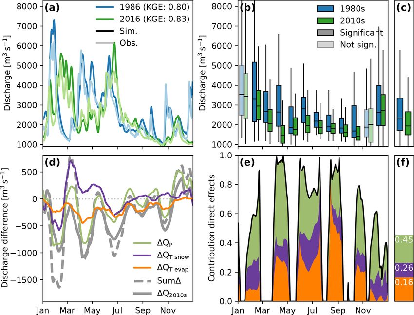
388                           J. Buitink et al.: Discharge response to temperature-driven changes in evaporation and snow

et al., 2013; Wang et al., 2010). With increased potential         cesses (snowfall and snowmelt and melt from glaciers). We
evaporation rates, discharge is expected to decrease. Sev-         test our main hypotheses that both seasonal changes in snow
eral recent studies have investigated the discharge response       processes and enhanced evaporation will aggravate low flows
to increased temperatures and generally expect lower dis-          and that the changes will increase with temperature under re-
charges resulting from increased evaporation and a shifted         alistic warming. We simulate the Rhine Basin at high spa-
seasonality induced by the changed snow dynamics (Milly            tial (4 km) and temporal (1 h) resolution using a calibrated
and Dunne, 2020; Mastrotheodoros et al., 2020; Rottler et al.,     version of the computationally efficient dS2 model, which is
2020). However, the relative importance and the combined           based on the simple dynamical-systems approach (Kirchner,
effect of evaporation and snow processes (including snowfall       2009; Teuling et al., 2010). The model was run for 2 decades
and snowmelt and melt from glaciers) on discharge and its          and for several scenarios with increased temperatures to un-
seasonal variability are currently not well understood.            derstand both historic changes and potential changes in the
   Europe has experienced significant changes in evapora-          future. The simulations performed at this rather unusually
tion, snow depth, and streamflow over the last decades. For        high temporal resolution ensure that diurnal variations – vi-
example, Teuling et al. (2019) showed that potential evapora-      tal for evaporation and snow processes – are correctly repre-
tion has increased by about 10 % over the period 1960–2010.        sented. By separating the temperature-driven effects on evap-
Their study shows that both changes in precipitation and           oration and snow processes, we can understand and quantify
evaporation had considerable effects on the streamflow. Ad-        the relative importance and interaction of each process.
ditionally, a study by Fontrodona Bach et al. (2018) showed
that snow depth has decreased over the majority of Europe
since the 1950s. Europe contains several major river basins of     2     Methods
high socio-economic importance. One of these is the Rhine
Basin, with its headwaters originating from the Alpine re-         2.1    Study area
gion. This basin covers many different types of land cover:
                                                                   This Rhine Basin is one of the major basins situated in north-
from glaciers to lowland areas. Several studies have already
                                                                   western Europe, covering several countries (see Fig. 1, also
investigated the response of this basin under different climate
                                                                   for typical climatic values). We focus on the basin upstream
scenarios (e.g. Stahl et al., 2016; te Linde et al., 2010; Hurk-
                                                                   of the Netherlands, as this river is of vital importance for
mans et al., 2010; Pfister et al., 2004; Shabalova et al., 2003;
                                                                   the country (e.g. agriculture, shipping). The basin includes
Middelkoop et al., 2001). Yet none of the studies have inves-
                                                                   part of the Alps, including several glaciers. Despite this be-
tigated the separate and combined response of evaporation
                                                                   ing only a small fraction of the basin (as can be inferred from
and snow processes to rising temperatures.
                                                                   the digital elevation model in Fig. 1a), it has considerable
   Spatially distributed modelling becomes increasingly vi-
                                                                   effects on the discharge (Stahl et al., 2016). As a result, a
able, due to the increased computational power, gains in
                                                                   correct understanding of temperature-driven changes is im-
model performance when adding spatial information (Co-
                                                                   portant to provide reliable discharge predictions. Despite dif-
mola et al., 2015; Lobligeois et al., 2014; Ruiz-Villanueva
                                                                   ferences in hydrological, climatic, and geological character-
et al., 2012), and increased availability of high-resolution
                                                                   istics, the discharge of many basins depends on meltwater
data (e.g. Huuskonen et al., 2013; Cornes et al., 2018;
                                                                   from snow and ice (Immerzeel et al., 2020). Therefore, we
van Osnabrugge et al., 2017; Hersbach et al., 2018). How-
                                                                   expect results from this study to give insight into the general
ever, the choice of spatial resolution can affect the model
                                                                   hydrological response to higher temperatures.
parameters (Melsen et al., 2016) and the sign of the simu-
lated anomalies (Buitink et al., 2018). Besides, when finer
spatial resolutions are used, the time step should be reduced      2.2    Models and data
as well, as the space and time dimensions are linked (Blöschl
and Sivapalan, 1995; Melsen et al., 2016). However, simu-          We used the computationally efficient distributed dS2 model
lations run at high spatial (and temporal) resolutions usu-        (Buitink et al., 2020) to simulate discharge in the Rhine
ally greatly increase computational demand (for example, the       Basin. The model is based on the simple dynamical-systems
study by Mastrotheodoros et al. (2020) on a 250 m resolu-          approach (Kirchner, 2009) and is extended with snow and
tion required more than 6 × 10⁵ CPU hours). This not only          routing modules. As dS2 requires actual evaporation data as
requires the use of high-performance clusters, but also has        input, we ran a soil moisture model (BETA, Beta Evapo-
the undesirable side effect of increased power consumption         Transpiration Adjustment) prior to the rainfall runoff model
(Loft, 2020). There is need for innovative hydrological mod-       to simulate the translation from potential evaporation (PET;
els which can run on high spatio-temporal resolution without       calculated using the Penman–Monteith equation, Monteith,
excessive computational demands, such as the recently de-          1965) to actual evaporation (AET). Since root zone depth
veloped dS2 model (Buitink et al., 2020).                          is an important yet highly uncertain parameter, we included
   This study investigates the hydrological response to            simulations with root zone depths ranging from 25 to 125 cm,
temperature-driven changes in evaporation and snow pro-            with increments of 25 cm. All simulations are performed at

Earth Syst. Dynam., 12, 387–400, 2021                                                  https://doi.org/10.5194/esd-12-387-2021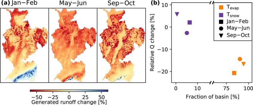
J. Buitink et al.: Discharge response to temperature-driven changes in evaporation and snow 389
Figure 1. Digital elevation model of the Rhine, and hydro-meteorological changes between the 1980s and the 2010s. Panel (a) shows the
simulation domain, with white lines indicating the main river branches. The red diamond indicates the location of the main outlet, and the red
star indicates the location of the Rietholzbach research catchment using for validation. Inset shows the location of the basin within Europe.
Panels (b), (c), and (d) show the yearly average values of the 1980s for temperature, precipitation, and potential evaporation, respectively,
and panels (e), (f), and (g) show the differences between the 1980s and the 2010s.
a resolution of 4 × 4 km and at an hourly time step. The two 2.2.1 BETA
models are explained in more detail below.
A simple soil moisture model (BETA, Beta EvapoTranspira-
The input data were obtained from the ERA5 reanaly-
tion Adjustment) is used to preprocess the evaporation input.
sis dataset (Hersbach et al., 2018). This dataset is globally
This model simulates the root zone and determines evapora-
available at a 0.25 × 0.25◦ resolution and at an hourly time
tion reduction based on the amount of water stored in the root
step from 1979 to present. ERA5 data were interpolated to
zone. Actual evaporation is assumed to be a function of the
the model grid using bilinear interpolation. We selected two
available soil moisture such that
periods with equal length based on the maximum distance
between available decades of ERA5 data: 1980–1989 and
ETactual = ETpotential · β(θ ), (1)
2009–2018, referred to as the 1980s and 2010s, respectively.
Soil data were obtained from the European Soil Hydraulic where β represents the evaporation reduction parameter as a
Database (EU-SoilHydroGrids ver1.0, Tóth et al., 2017). function of soil moisture θ . β is defined using three linear
As this dataset did not contain critical soil moisture con- relations with θ , based on Laio et al. (2001):
tent needed by the model to distinguish between water- and
energy-limited evaporation regimes (Denissen et al., 2020),
θ −θ
h
βw θw −θh
if θ ≤ θw
it was determined as the mean between wilting point and θ−θ
β(θ ) = βw + (1 − βw ) θ −θ w
if θw ≤ θ ≤ θc (2)
field capacity. The hygroscopic moisture content was calcu- c w
1 if θc ≤ θ ≤ θs ,
lated from the moisture retention curve based on Mualem–
van Genuchten parameters at −10 MPa (Laio et al., 2001;
Tóth et al., 2017). The clay content of the European Soil Hy- where βw represents the evaporation reduction factor at wilt-
draulic Database was used to calculate the pore size distri- ing point (set to 0.1), θh represents the hydroscopic point, θw
bution (b) through a linear fit of the values found in Clapp the wilting point, θc the critical soil moisture content, and θs
and Hornberger (1978). For the depth of the root zone, we the saturated soil moisture content.
chose a depth of 75 cm but also included simulations rang- Leakage from the root zone is calculated to simulate the
ing from 25 to 125 cm with increments of 25 cm to account vertical movement of water. This water is assumed to be gone
for the uncertainty of this parameter. The potential evapora- from the root zone, as we do not simulate a layer below the
tion input data were calculated using the Penman–Monteith root zone. The leakage is based on the unit-gradient assump-
equation (Monteith, 1965), based on ERA5 input data. tion in combination with the Clapp and Hornberger (1978)
model for unsaturated conductivity, integrated over a time
https://doi.org/10.5194/esd-12-387-2021 Earth Syst. Dynam., 12, 387–400, 2021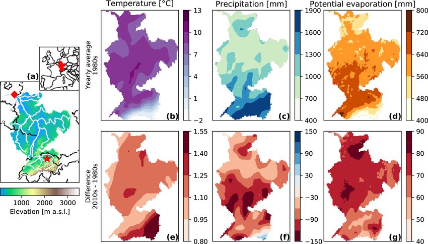
390                               J. Buitink et al.: Discharge response to temperature-driven changes in evaporation and snow

step 1t:                                                                  step. This snow module is conceptualized as follows (as de-
                                                                          fined by Buitink et al., 2020):
Qleakage
                                                                          dSsnow
               "        −2b−2                     #−     1                     = Psnow − Msnow ,                                   (9)
                    θt              (2b + 2)ks 1t        2b+2               dt
 = Lθt − Lθs                      +                             ,   (3)            (
                    θs                  θs L                                        Ptotal if T  T0 ,
where L represents the depth of the root zone, θt the soil                         (
moisture content at time step t, b the pore size distribution,                      ddf · (T −T0 ) if Msnow · 1t  Ssnow ,
lated through the clay fraction (CF), using a linear fit based
                                                                          where Ssnow is the total snow storage in millimetres (mm),
on the values in Clapp and Hornberger (1978):
                                                                          Psnow is the precipitation falling as snow in millimetres per
b = 13.52 · CF + 3.53.                                              (4)   hour (mm h−1 ), Msnow is the snowmelt in millimetres per
                                                                          hour (mm h−1 ), T is the air temperature in degrees Celsius
   Finally, the water balance for the root zone is defined as             (◦ C), T0 is the critical temperature for snowmelt in degrees
follows:                                                                  Celsius (◦ C), ddf is the degree-day factor in millimetres per
                                                                          hour per degree Celsius (mm h−1◦ C−1 ), and 1t is the simu-
θt+1 = θt + 1t(Prain + Msnow − ETactual − Qleakage ),               (5)   lation time step in hours. We define separate melt factors for
                                                                          snow and glaciers. Partitioning of precipitation between liq-
where Prain is the rate of rainfall at time step t, Msnow the rate        uid and solid precipitation (rain and snow) and melt is based
of snowmelt at time step t, and both are inferred in the same             on the critical temperature (set to 0 ◦ C). Routing of water is
way as in the dS2 model (see below and Buitink et al., 2020).             based on the width function (Kirkby, 1976), which means
                                                                          that lakes and other hydraulic structures are not explicitly
2.2.2   dS2                                                               simulated. More details on the routing module can be found
                                                                          in Buitink et al. (2020).
A conceptual rainfall–runoff model is used to simulate the
                                                                             To calibrate dS2, we optimized the three discharge sensi-
discharge in the Rhine Basin. The dS2 model (Buitink et al.,
                                                                          tivity parameters, the degree-day factor for both snow and
2020) is based on the simple dynamical-systems approach,
                                                                          glacier pixels, and an evaporation correction factor. The
as proposed by Kirchner (2009). This approach is based on
                                                                          evaporation correction factor is included to correct any bias
the assumption that discharge is a function of storage, such
                                                                          errors in the forcing data. According to Boussinesq’s theory
that changes in storage can be related to changes in discharge
                                                                          of sloping aquifers (Rupp and Selker, 2006) and the results
via a discharge sensitivity function:
                                                                          found in Karlsen et al. (2019), systems with higher slopes are
 Q = f (S),                                                         (6)   expected to show higher discharge sensitivity values. There-
                                                                          fore, the discharge sensitivity parameters were defined as a
dQ dQ dS      dQ
   =        =    (P − ET − Q),                                      (7)   linear function of the slope of each pixel, based on the hy-
dt   dS dt    dS                                                          pothesis that regions with steeper slopes show a more re-
where Q represents the discharge, S the storage, P and ET                 sponsive storage–discharge relation than regions with gen-
the precipitation and actual evaporation, respectively, and dQ
                                                            dS
                                                                          tle slopes. This resulted in two fitting parameters (slope and
the discharge sensitivity to changes in storage, referred to as           intersect) for each of the three discharge sensitivity param-
g(Q). This concept has been successfully applied and vali-                eters. Latin hypercube sampling was used to gain parameter
dated in several catchments across Europe (Kirchner, 2009;                values evenly sampled across the possible parameter space.
Teuling et al., 2010; Krier et al., 2012; Brauer et al., 2013;            The period 2004–2008 was used for calibration. To ensure re-
Melsen et al., 2014; Adamovic et al., 2015). Buitink et al.               alistic model performance across the entire basin, the Kling–
(2020) further developed the concept so it can be applied in a            Gupta efficiency (KGE; Kling and Gupta, 2009) was calcu-
distributed way, to allow the simulation of larger catchments,            lated at 13 discharge measurement stations within the Rhine
while respecting the original scale of development. A new                 Basin (see Supplement for corresponding locations and per-
equation to better capture the typical shape of the g(Q) re-              formance metrics). KGE values across all stations are aver-
lation is proposed by Buitink et al. (2020), which contains               aged, and the parameters from the run with the best aver-
three parameters:                                                         age KGE are selected. The resulting parameter values can be
                                                                          found in the Supplement.
g(Q) = eα+β ln(Q)+γ /Q .                                            (8)
                                                                          2.3   Experimental setup
  Additionally, the model has been extended with a snow
module based on Teuling et al. (2010). The snow module is                 We have split our analysis into two parts. Firstly, we compare
based on a degree-day method, adjusted to the hourly time                 2 decades to understand the relative impact of each forcing

Earth Syst. Dynam., 12, 387–400, 2021                                                       https://doi.org/10.5194/esd-12-387-2021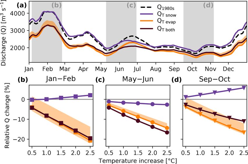
J. Buitink et al.: Discharge response to temperature-driven changes in evaporation and snow                                  391

variable. Secondly, we increase temperature values with 0.5◦     experimental setup is, to our knowledge, new and has not
increments to understand how an increase in temperature af-      yet been applied in other studies. It allows us to understand
fects the hydrological response in the Rhine Basin. We ex-       changes directly driven by a change in forcing, but quanti-
plain both experiments in more details below.                    fying combined changes remains challenging (e.g. change in
                                                                 type of precipitation due to the interaction of precipitation
2.3.1   Validation
                                                                 and temperature). The resulting simulated discharge is com-
                                                                 pared to the 1980s run, to determine the discharge change. In
A thorough validation is required in order to ensure that mod-   this way, we can evaluate the relative impact of each forcing
els simulate the correct sign and magnitude of the trends        variable on the discharge.
(Melsen et al., 2018). Therefore, we validated dS2 on three         We sum the discharge changes in the three forcing-
variables: discharge of the total catchment and snow and         swapped runs, to obtain Sum1 (as time series):
evaporation dynamics. Additionally, the validation of snow
and evaporation is performed at two levels: local tempo-         Sum1 = 1QP + 1QT snow + 1QT evap ,                          (12)
ral validation with point observations from the Rietholzbach
research catchment (Seneviratne et al., 2012) in Switzer-        where 1Qx represents the discharge difference of the
land (location is indicated with the red star in Fig. 1a)        forcing-swapped simulations. We can use this Sum1 to
and spatial validation of evaporation and snow patterns us-      study how well it explains the 2010s run, by comparing it
ing GLEAM (v3.3, Martens et al., 2017) and the Euro-             to 1Q2010s . We hypothesize that when Sum1 is equal to
pean Climate Assessment & Data Set (ECA&D; Tank et al.,          1Q2010s , the effect of the forcing is additive and together
2002; Fontrodona Bach et al., 2018). The Rietholzbach re-        explains all differences. We will refer to this as the direct
search catchment was selected as the data are available at a     effects. In the case of a discrepancy between Sum1 and
high temporal resolution (hourly), which matches our model       1Q2010s , this can be attributed to the interaction between
setup. Snow observations from both the Rietholzbach and          the three forcing components. We will refer to this as indi-
ECA&D are reported as snow depth, where dS2 simulates            rect effects. For example, temperature and precipitation are
snow water equivalent. In the graphs, we assume a transfor-      linked as the type of precipitation (rain or snow) is depen-
mation factor of 0.1 (where 10 mm of snow depth represents       dent on temperature (see Eq. 10): a precipitation event in the
1 mm of snow water equivalent) but always show both axes.        1980s would be falling as snow with the temperature of the
                                                                           1980s ). When we swap T 1980s with T 2010s , the same
                                                                 1980s (Tsnow
The ECA&D dataset only contains point observations, and                                             snow        snow
no stations in France are available. Due to data availability    event could be classified as liquid rain leading to a direct
limitations of the Rietholzbach catchment, we had to resort      runoff response, as opposed to the original snowfall event
to our calibration period. Since dS2 was only calibrated on      with snowmelt later in the year. This could also happen vice
discharge, this can still be interpreted as validation.          versa or with swapped precipitation time series. The forcing-
                                                                 swapped simulations do not capture these interactions.
                                                                    We define Sum1 to have explanatory value when it has
2.3.2   Forcing swap
                                                                 the same sign as 1Q2010s . We calculate the contribution of
In the first experiment, we aim to understand how each forc-     the direct effects (φ) using the following equation:
ing variable can explain the resulting changes in discharge,           min(Sum1,1Qall )
and their relative importance. To perform this, we set up                max(Sum1,1Qall )   if sign(Sum1) = sign(1Qall )
                                                                 φ=                                                          (13)
the experiment according to the conceptual overview pre-                 0                  if sign(Sum1) 6= sign(1Qall ).
sented in Fig. 2. The first two simulations are straightfor-
ward: using all forcing variables from either the 1980s or       This value can then be used to calculate the relative (direct)
the 2010s to produce the corresponding discharge time series     contribution of each forcing variable, using the following
(“1980s” and “2010s”). In order to investigate how tempera-      equation:
ture influences evapotranspiration and snow processes sepa-
rately, we perform model runs in which the total temperature     φx
change is separated into temperature effects on evapotran-                            abs(1Qx )
                                                                 =                                                 · φ, (14)
spiration (“Changed Tevap ”) and snow processes (“Changed             abs(1QP ) + abs(1QT snow ) + abs(1QT evap )
Tsnow ”). In addition, another run is performed with only
changes in P (“Changed P ”), so that these individual runs       where 1Qx should be replaced by 1QP , 1QT snow , or
can be compared to a run where all changes in forcing are        1QT evap .
enabled (“2010s”). The Changed Tevap simulation changes
the amount of evaporation which results from the new tem-        2.3.3       Increased temperatures
perature time series. For the Changed Tsnow simulation, the
following snow processes are affected: type of precipitation     In the second experiment, we raise temperature in 0.5 ◦ C
(rain or snow), melt from snow, and melt from glaciers. This     increments to understand how the basin responds to higher

https://doi.org/10.5194/esd-12-387-2021                                               Earth Syst. Dynam., 12, 387–400, 2021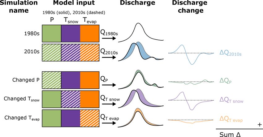
392 J. Buitink et al.: Discharge response to temperature-driven changes in evaporation and snow
Figure 2. Conceptualization of the forcing swap experiment, showing the different simulations (rows) and steps in the analysis (columns).
The different forcing variables are visualized as coloured blocks, where the solid and dashed boxes indicate forcing data from the 1980s and
the 2010s, respectively.
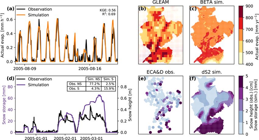
temperatures. We use the 1980s period as a baseline and in- Discharge validation (Fig. 3a) shows that dS2 simulates
crease the temperature until 2.5 ◦ C, to match realistic tem- the discharge with high KGE values in both periods. Panel
perature projections. Similar to the previous experiment, we b shows how the average discharge differs between the two
separate the effects of temperature on evaporation and snow periods, with lower discharges in the 2010s for the majority
processes: an increase in Tevap influences the resulting evap- of the year. Discharge during the 2010s does not show as high
oration, where an increase in Tsnow affects the type of precip- discharge values in June and shows lower discharge values
itation and the melt from snow and glaciers. By separating occurring later in the year. Kling–Gupta efficiencies for each
these effects, we can understand their relative importance for period and several stations within the basin can be found in
each temperature increase. This is a simplified approach, as the Supplement (Table S1).
a recent study by van der Wiel and Bintanja (2021) showed For the validation with data from the Rietholzbach catch-
that a warming climate affects not only the mean, but also the ment, we compare simulated actual evaporation with ob-
variability. The latter is not captured in our approach. served evaporation from a lysimeter and compare simu-
lated snow storage with observed snow height measure-
ments in Fig. 4. Both variables are correctly represented
and show similar variability as the observations, even at an
3 Results
hourly timescale. The simulated evaporation generally shows
a smoother signal than the observations. Snow storage shows
3.1 Forcing comparison and validation a very similar pattern. It has to be noted that snow height
observations cannot be directly converted into snow water
A first comparison of average temperature, precipitation, and
equivalent, due to, e.g., compaction. Yet dS2 simulates melt
potential evaporation reveals considerable differences be-
and snowfall at moments corresponding with observations, as
tween the two periods (Fig. 1). Over the entire Rhine Basin,
is confirmed by the contingency table in panel b. Given that
yearly average temperature has increased by more than 1 ◦ C,
dS2 is not calibrated on these variables and given the differ-
from 8.1 to 9.3 ◦ C between the 1980s and 2010s. The largest
ence in spatial scale of the input data, this shows that dS2 is
differences are found in the eastern Alps, where average tem-
able to correctly simulate evaporation and snow processes.
perature has risen by 1.5 ◦ C (Fig. 1b, e). Average precipi-
This is confirmed in the spatial validation, where we com-
tation is lower in the 2010s over the majority of the Rhine
pare the actual evaporation results from the BETA model
Basin, with the yearly average precipitation sums decreas-
with results from GLEAM (Martens et al., 2017). We see
ing from 1146 to 1066 mm (Fig. 1c, f). Spatial differences in
some deviations in terms of magnitude, where BETA simu-
precipitation are, however, less homogeneous over the basin
lates slightly higher values than GLEAM. However, despite
than the changes in temperature and potential evaporation.
the differences in spatial resolution, the patterns are well rep-
As a result of the increased temperatures, average potential
resented in BETA: higher values in the southern region of the
evaporation also substantially increased from 607 to 678 mm
basin, with lower values in the central or northern regions.
from the 1980s to the 2010s, with the largest increases occur-
The simulated snow storage is compared with observations
ring in the northern parts of the basin (Fig. 1d, g).
Earth Syst. Dynam., 12, 387–400, 2021 https://doi.org/10.5194/esd-12-387-2021J. Buitink et al.: Discharge response to temperature-driven changes in evaporation and snow 393
Figure 3. Attribution of discharge changes between the 1980s and the 2010s. Panel (a) compares simulated (dark colours) with observed
(light colours) discharge values for 1 representative year in each period. Panels (b) and (c) compare the monthly and yearly (respectively)
simulated discharge values between the two periods, where fully coloured boxes are significantly different (p < 0.05, based on independent
t test). Panel (d) shows the difference of model simulations where one of the forcing time series of the 1980s has been swapped with the time
series from the 2010s. Panel (e) shows the contribution of direct effects (black line) and the contribution of each forcing variable to the total
change between the two periods. Overall mean values of the time series in (e) are presented in (f).
from the ECA&D dataset, provided by Fontrodona Bach shows higher discharge values resulting from a more direct
et al. (2018). It should be noted that the observations are discharge response due to more rain (instead of snow) and en-
measured as snow height, while dS2 simulates snow water hanced melt from the glaciers. From July onwards, discharge
equivalent. The figure shows that dS2 simulates snow cover values converge back to the original 1980s simulation, in-
with a similar pattern as is observed: with high values in the dicating that the discharge regime becomes less dominated
Alps and south-eastern region and low values in the central by melt from snow and ice. The simulation with evaporation
and northern parts of the basin. from the 2010s (1QT evap ) shows a discharge reduction over
the entire year. The higher PET leads to higher actual evapo-
3.2 Forcing swap ration, decreasing the discharge.
The contribution of direct effects in Fig. 3e–f gives an
Investigating the differences between the “forcing-swapped” indication of the amount of interaction between the three
runs gives insight into how each variable affects the discharge forcing variables. Values close to 1 indicate that there is lit-
(see Fig. 3d, e, and f). Changing the precipitation (1QP ) has tle interaction, as the sum of the differences is able to ex-
substantial effects on the discharge (Fig. 3d), swinging from plain all changes. The contribution of direct effects is low-
large negative discharge differences to positive differences. est during March and around October. During these periods,
This is not unexpected, as precipitation is the factor control- the storage conditions of the basin largely control the dis-
ling water input into the basin. Changing only the tempera- charge response, either through snow storage or water avail-
ture related to snow processes (1QT snow , including the type able to generate runoff. Around March, changes in the avail-
of precipitation and melt from snow and glaciers) shows dis- able snow storage are the result of interactions between tem-
charge differences mostly in the first half of the year. The perature and precipitation. Around October, discharge is con-
reduction in discharge in January and February is caused by trolled by water that is available for runoff generation, which
overall higher temperatures: less precipitation has fallen as is controlled by interactions of precipitation and evaporation.
snow in the preceding months (as inferred from the increased Additionally, since the response of a pixel is a function of its
discharge at the end of the year), leading to less snowmelt in storage (through the simple dynamical-systems approach),
January and February. From March to May, this simulation
https://doi.org/10.5194/esd-12-387-2021 Earth Syst. Dynam., 12, 387–400, 2021394 J. Buitink et al.: Discharge response to temperature-driven changes in evaporation and snow
Figure 4. Temporal and spatial validation of evaporation rates (a, b, c) and snow storage (d, e, f). Panels (a) and (d) show validation with
observations from the Rietholzbach research catchment (location can be found in Fig. 1a), with the table in (d) showing the contingency table
with the percentage of occurrences with snow (S) and with no snow (NS). Note that panel (d) has two y axes: snow storage for the simulation
and snow height for the observations. Panels (b) and (c) show the annual mean actual evaporation of 2005 as determined with both GLEAM
and BETA (with a rooting depth of 75 cm). Panels (e) and (f) show annual mean snow heights of 2005, as observed in the ECA&D dataset
(snow height in cm) and simulated with dS2 (snow storage in mm).
this also affects the runoff response. These interactions of ing typical discharge regimes: high discharge during January
forcing variables cannot be captured by simply combining and February, the meltwater peak during May and June, and
the individual discharge responses, hence the relatively large low discharge during September and October. For each of
contribution of indirect forcing effects during these periods. these periods, the change in discharge shows a roughly lin-
When taking the averages of the values in Fig. 3e, the results ear relation with temperature increase. This is in line with
show (Fig. 3f) that, overall, it is possible to explain almost our hypothesis that higher temperatures will lead to larger
half of the 2010s discharge scenario by the direct forcing ef- differences in discharges. The resulting near-linear relation
fects. The temperature effects of evaporation and snow (0.16 is interesting, as both snow and evaporation processes are
and 0.10, respectively, totalling 0.26) are just as important threshold processes through their relation with temperature
as the changes induced by differences in precipitation (0.19), and soil moisture, respectively. We expect to see a more non-
yet due to the large role of interactions, no more than 45 % linear response to temperature when reaching more hydro-
can be explained using this simple addition. logical extremes.
Surprisingly, for the periods during January–February and
September–October (Fig. 5b and d), the modified snow run
3.3 Increased temperatures shows behaviour that is the opposite of both the modified
In the second experiment, we investigate the role of temper- evaporation run and the combined run. In these cases, the
ature increases in changes in discharge. Higher temperatures increased discharge as result of a change in snow processes
affect the hydrological cycle through evaporation, snow pro- (more liquid precipitation, and more meltwater production
cesses (snowfall and melt from snow and ice), or a combined from the glaciers) slightly offsets the negative discharge
effect of the two. Using the dS2 model, separate simula- change induced by the increased evaporation. This ensures
tions of temperature effects on evaporation (QT evap ), snow that the combined reduction in discharge is less severe than
(QT snow ), and their combined effect (QT both ) allow us to un- when only the reduction induced by evaporation is consid-
derstand which variable is causing the main changes. These ered. However, during May–June (Fig. 5c), both evaporation
time series are presented in Fig. 5a, including the 1980s run and snow processes show a negative discharge change, en-
as a reference. Throughout the year, we see a near-constant hancing the combined negative change in discharge. During
reduction in discharge, without clear seasonal patterns. To in- this period, less snow was available to melt, leading to a re-
vestigate this further, we highlighted three periods represent- duction in discharge. As a result, the discharge of the com-
Earth Syst. Dynam., 12, 387–400, 2021 https://doi.org/10.5194/esd-12-387-2021J. Buitink et al.: Discharge response to temperature-driven changes in evaporation and snow 395
where neither snow nor evaporation appeared dominant take
up only a very small fraction of the basin (< 1 %). Generally,
these regions are at the transition between snow-dominated
and evaporation-dominated regions. Overall, the change in-
duced by Tsnow – despite the small contributing area – sub-
stantially affects the discharge. More details on the response
for each temperature increase can be found in the Supple-
ment.
4 Discussion
We compared two periods of 10 years to investigate the rela-
tive importance of changes in temperature, evaporation, and
Figure 5. Discharge sensitivity to temperature increase. Panel (a) precipitation. Over these periods of 10 years, most interan-
shows the yearly average discharge under a 2.5 ◦ C increase, and nual variability is averaged out, allowing us to objectively in-
panel (b) shows changes during typical discharge events with step- vestigate the effect of different temperatures on the hydrolog-
wise temperature increases. Typical discharge periods highlighted ical response. However, decadal variation remains present,
in (a) match the periods used to compare the mean discharges in (b, but due to the length of these periods, it is not possible to
c, d). Shaded orange areas indicate the uncertainty induced by ef- fully contribute these changes to a change in climate.
fective rooting depth (25–125 mm), where higher discharges match When validating the model with data from the Ri-
shallower depths and vice versa. etholzbach, the simulated evaporation in the Rietholzbach
showed a smoother signal than the observations. Deviations
between the observations and simulations could be caused by
bined run shows an even larger reduction in discharge, where the relatively coarse ERA5 data. Especially in the spatially
even the peak during June from the 1980s has been largely di- heterogeneous Alps, a single ERA5 pixel could miss some
minished (Fig. 5a). The exact response of the type of precip- local variations (such as variations in cloud cover, radiation,
itation, snow depth, cover, and melt, and melt from glaciers wind, and/or temperature), causing a smoother signal in the
for each temperature increase can be found in the Supple- simulated evaporation. For the spatial evaporation validation
ment. A substantial influence of rooting depth on the evap- with GLEAM, it should be noted that this is not a true valida-
oration simulation is visible (shaded orange areas in Fig. 5), tion, since GLEAM is not a completely independent observa-
yet the trend direction with increasing temperatures remains tional dataset. Despite this, GLEAM is often considered as a
equal. Shallower rooting depth values induce more soil mois- reference for spatio-temporal validation of ET. Additionally,
ture stress since less water is available, leading to higher av- BETA uses a single rooting depth value for the Rhine Basin.
erage discharges. The choice of spatial model resolution is a balance be-
To understand the cause of these changes, the change in tween data availability, computational time, and underly-
generated runoff per model pixel is shown in Fig. 6a. This ing modelling concept. Here we selected a resolution of
figure shows that the majority of the basin produces less 4 × 4 km, so we can use the ERA5 forcing data with bilinear
runoff for all three periods. Only the southern regions of the resampling (without adding more degrees of freedom, uncer-
basin show a different response. During January and Febru- tainty, and potential errors), have short run times (simulat-
ary, these regions produced more runoff, resulting from the ing 10 years including all input/output operations takes just
increased snowmelt and increased liquid precipitation. In the over 5 min on a normal desktop), and apply the model at its
other periods, only a few pixels produced more runoff. These proven spatio-temporal scale (±10 km2 at hourly time step).
pixels correspond to the glaciers in the Alps, which produced By contrast, the study by Mastrotheodoros et al. (2020) used
more meltwater resulting from the increased temperatures, a much finer spatial resolution but at the cost of enormous
and explain the positive discharge change in Fig. 5d. CPU times.
In Fig. 6b, the fraction of the basin that is dominated Several other recent studies have investigated the hydro-
by one of these three options is plotted against the relative logical response to increased temperatures via either changes
change in mean discharge for each period. As expected, the in evaporation and/or snow processes (snowfall and melt
majority of the basin is mainly influenced by evaporation from snow and ice). Below, we compare our results with
(84 %–94 %). As a result, the mean discharge is reduced by the results found in three of these studies. Firstly, the study
±17 %. By contrast, a limited fraction of the basin (1 %– by Rottler et al. (2020) showed a decrease in runoff season-
6 %) is mainly influenced by snow processes, yet still has a ality in rivers fed by meltwater from snow over the period
considerable effect on the mean discharge, varying between 1869–2016. They found higher discharges during winter and
−3 % and 6 %, depending on the period. Pixels in the basin spring and lower discharges during summer and autumn. The
https://doi.org/10.5194/esd-12-387-2021 Earth Syst. Dynam., 12, 387–400, 2021396 J. Buitink et al.: Discharge response to temperature-driven changes in evaporation and snow Figure 6. Spatial differences in the Rhine Basin under the +2.5 ◦ C scenario. Panel (a) shows the differences in generated runoff for the three periods highlighted in Fig. 5a. Panel (b) shows the fraction of the basin where 80 % of the changes could be explained by either evaporation or snowmelt and the average discharge change corresponding to each process. authors conclude that reservoir constructions in these snow- means that, under increased temperature scenarios, snowmelt dominated rivers are likely to cause this redistribution of dis- occurs on days where previously no melt was possible. Addi- charge. However, our temperature experiment shows a sim- tionally, dS2 does simulate earlier depletion of the snowpack, ilar change in discharge: with higher discharges in winter which also reduces snowmelt rates. Despite our different aim and spring and lower discharges during summer. As the dS2 and approach, we believe that our study supports the findings model does not include dams and other reservoirs, this sig- of Musselman et al. (2017). nal can be attributed to a change in discharge production. The glaciers used in our model are fixed in space, and no Secondly, a recent study investigating the response of sev- growing or shrinking of glaciers is simulated. While the ap- eral basins in Czechia to changes in snowmelt concluded that proach is common for shorter-timescale studies such as ours snowmelt started earlier in the year, which also reduced sum- (van Tiel et al., 2018), it limits the interpretation of our re- mer low flows via baseflow (Jenicek and Ledvinka, 2020). sults several decades into the future. The study by Lutz et al. However, our study shows that low flows during Septem- (2014) included a glacier mass balance and showed that melt ber and October actually increased when only snow pro- from glaciers increased before the glaciers eventually disap- cesses are considered. This can be explained by that fact pear. Without glaciers, increases in drought severity are ex- that the Rhine Basin includes glaciers, which produce more pected, as less meltwater is produced during the summers meltwater with higher temperatures (assuming the glacier is (van Tiel et al., 2018; Huss, 2011). After 2050, substan- thick enough to facilitate this melt). This increase in melt- tial changes in summer flow resulting from the reduction in water resulted in higher discharge volumes during summer. glacierized area are expected (Huss, 2011). Until this period, Thirdly, Milly and Dunne (2020) showed a reduction in dis- we expect our results to be representative. charge in the Colorado River basin and conclude that this When comparing our results with results from studies per- is driven by increased evaporation. This increase in evapo- formed in the Rhine Basin (e.g. te Linde et al., 2010; Hurk- ration is attributed to a reduction in snow cover and hence mans et al., 2010; Pfister et al., 2004; Shabalova et al., 2003; a decreased albedo. Despite the different basin, our study Middelkoop et al., 2001), we see similar results. These stud- supports the conclusion that increased temperatures reduce ies focussed mainly on understanding and/or projecting the discharge through both changes in snow processes and in- Rhine discharge under climate scenarios. Yet all these stud- creased evaporation. Our model does not account for changes ies agree that the snowmelt peak will occur earlier in the year in albedo but does allow areas previously covered in snow to and that the basin is expected to transition from a mixed rain- evaporate water. And while differences in climate zone be- and snow-fed river to a mostly rain-fed river. Additionally, tween the Colorado and Rhine basins make it challenging to all studies agree to expect higher evaporation rates, further compare the absolute numbers, the sign of the trend is equal. reducing the discharge. This is all in line with our study, de- Musselman et al. (2017) concluded that there was a low- spite the fact that we did not investigate changes in precipi- ering of snowmelt rates due to a shift in the melt season to- tation in our temperature scenarios. Furthermore, the Rhine wards a period with lower available energy (spring instead Basin contains several hydraulic control measures, which are of summer). They simulated the snowpack with a more com- currently not represented in our model structure. Despite this, plex energy balance rather than our degree-day method. The we still reach good model performance, suggesting that these dS2 model does not include the radiation-driven changes but structures currently do not have a very large influence on the does simulate that snowmelt occurs earlier in the year. This discharge dynamics at the basin outlet. In the future, how- Earth Syst. Dynam., 12, 387–400, 2021 https://doi.org/10.5194/esd-12-387-2021
J. Buitink et al.: Discharge response to temperature-driven changes in evaporation and snow                                           397

ever, the management schemes and number of structures can         Code and data availability. Model code and information is
be altered to accommodate the changes in the hydrological         available at https://doi.org/10.5194/gmd-13-6093-2020 (Buitink
cycle. As these changes are a large unknown, we decided to        et al., 2020). Forcing data were obtained from https://cds.climate.
only focus on the natural hydrological response.                  copernicus.eu/cdsapp#!/home (Hersbach et al., 2018). Soil data
                                                                  were obtained from https://doi.org/10.1002/hyp.11203 (Tóth et al.,
                                                                  2017).
5   Conclusions
                                                                  Supplement. The supplement related to this article is available
Temperature, evaporation, and precipitation substantially
                                                                  online at: https://doi.org/10.5194/esd-12-387-2021-supplement.
changed from the 1980s to the 2010s in the Rhine Basin,
reflecting changes that are typical for many larger basins
around the world. In the 2010s, basin average temperature         Author contributions. JB and AJT designed the study. JB per-
was more than 1 ◦ C higher, potential evaporation was almost      formed the model simulations and analyses and wrote the paper
70 mm higher, and precipitation decreased with 80 mm. Dis-        with contributions from LAM and AJT.
charge between these two periods was significantly different
for 10 out of 12 months. Each individual forcing variable can
partly explain these discharge differences: 10 % can be ex-       Competing interests. The authors declare that they have no con-
plained by the changed snowfall and melt dynamics, 16 %           flict of interest.
is explained by the changed evaporation, and 19 % by the
changed precipitation, leaving 55 % to be explained by the
interaction of these variables. As differences in evaporation,    Acknowledgements. We would like to thank Christoph Brühl
snowfall, and melt are driven by changes in temperature, the      and Doke Schoonhoven for their work during their MSc theses,
temperature effect is larger (26 %) than the changes induced      which set the foundation for this study.
by changes in precipitation (19 %).
   With higher temperatures, discharge is expected to de-
crease, resulting from the positive effect of temperature on      Financial support. This research has been supported by Rijkswa-
                                                                  terstaat, the Directorate-General for Public Works and Water Man-
(potential) evaporation. However, snow processes (more liq-
                                                                  agement and part of the Ministry of Infrastructure and Water Man-
uid precipitation and enhanced melt from glaciers) can par-
                                                                  agement of the Netherlands.
tially offset the negative change in discharge during the
low flows in September–October, which was contrary to
our expectations. The discharge response during May–July          Review statement. This paper was edited by Gabriele Messori
matches our hypothesis that both changes in snow processes        and reviewed by three anonymous referees.
and evaporation enhance the reduction in discharge. This is a
result of the combined effect of enhanced evaporation and a
reduction in snowpack leading to less snowmelt.
   This study focusses on the Rhine Basin, yet these results
can provide insight for the many different basins around the      References
globe, which also depend on both rain- and snowfall. With
higher temperatures, changes in snow processes slightly off-
                                                                  Adamovic, M., Braud, I., Branger, F., and Kirchner, J. W.: Assess-
set the discharge reduction from enhanced evaporation over          ing the simple dynamical systems approach in a Mediterranean
the majority of the year. However, the season where runoff          context: application to the Ardèche catchment (France), Hydrol.
generation is reduced due to smaller snow stores (and po-           Earth Syst. Sci., 19, 2427–2449, https://doi.org/10.5194/hess-19-
tentially smaller glaciers) should be identified in each basin,     2427-2015, 2015.
as this part of the year is impacted the most. Many regions       Baraer, M., Mark, B. G., McKenzie, J. M., Condom, T., Bury, J.,
rely on water towers for their year-round water availabil-          Huh, K.-I., Portocarrero, C., Gómez, J., and Rathay, S.: Glacier
ity (Immerzeel et al., 2020), where the mountainous regions         recession and water resources in Peru’s Cordillera Blanca, J.
cover varying fractions of the basin. In many basins, more of       Glaciol., 58, 134–150, https://doi.org/10.3189/2012JoG11J186,
the discharge originates from these water towers than in the        2012.
                                                                  Beniston, M., Farinotti, D., Stoffel, M., Andreassen, L. M., Cop-
Rhine Basin, amplifying our results. Here, higher tempera-
                                                                    pola, E., Eckert, N., Fantini, A., Giacona, F., Hauck, C., Huss,
tures would likely imply even stronger negative amplitudes
                                                                    M., Huwald, H., Lehning, M., López-Moreno, J.-I., Magnusson,
in discharge trends during the melt season. Enhanced melt           J., Marty, C., Morán-Tejéda, E., Morin, S., Naaim, M., Proven-
from glaciers and a shift from snow to rain can partially off-      zale, A., Rabatel, A., Six, D., Stötter, J., Strasser, U., Terzago, S.,
set the negative change in discharge caused by the increased        and Vincent, C.: The European mountain cryosphere: a review of
evaporation but can enhance the negative change when snow           its current state, trends, and future challenges, The Cryosphere,
stores are eventually depleted earlier in the year.                 12, 759–794, https://doi.org/10.5194/tc-12-759-2018, 2018.

https://doi.org/10.5194/esd-12-387-2021                                                 Earth Syst. Dynam., 12, 387–400, 2021
398 J. Buitink et al.: Discharge response to temperature-driven changes in evaporation and snow Blöschl, G. and Sivapalan, M.: Scale issues in hydrolog- Huntington, T. G.: Evidence for intensification of the global ical modelling: A review, Hydrol. Process., 9, 251–290, water cycle: Review and synthesis, J. Hydrol., 319, 83–95, https://doi.org/10.1002/hyp.3360090305, 1995. https://doi.org/10.1016/j.jhydrol.2005.07.003, 2006. Brauer, C. C., Teuling, A. J., Torfs, P. J. J. F., and Uijlen- Hurkmans, R. T. W. L., Terink, W., Uijlenhoet, R., Torfs, hoet, R.: Investigating storage-discharge relations in a low- P., Jacob, D., and Troch, P. A.: Changes in streamflow land catchment using hydrograph fitting, recession analysis, dynamics in the Rhine basin under three high-resolution and soil moisture data, Water Resour. Res., 49, 4257–4264, regional climate scenarios, J. Climate, 23, 679–699, https://doi.org/10.1002/wrcr.20320, 2013. https://doi.org/10.1175/2009JCLI3066.1, 2010. Buitink, J., Uijlenhoet, R., and Teuling, A. J.: Evaluating seasonal Huss, M.: Present and future contribution of glacier hydrological extremes in mesoscale (pre-)Alpine basins at coarse storage change to runoff from macroscale drainage 0.5◦ and fine hyperresolution, Hydrol. Earth Syst. Sci., 23, 1593– basins in Europe, Water Resour. Res., 47, W07511, 1609, https://doi.org/10.5194/hess-23-1593-2019, 2019. https://doi.org/10.1029/2010WR010299, 2011. Buitink, J., Melsen, L. A., Kirchner, J. W., and Teuling, A. J.: Huuskonen, A., Saltikoff, E., and Holleman, I.: The Operational A distributed simple dynamical systems approach (dS2 v1.0) Weather Radar Network in Europe, B. Am. Meteorol. Soc., 95, for computationally efficient hydrological modelling at high 897–907, https://doi.org/10.1175/BAMS-D-12-00216.1, 2013. spatio-temporal resolution, Geosci. Model Dev., 13, 6093–6110, Immerzeel, W. W., Lutz, A. F., Andrade, M., Bahl, A., Biemans, H., https://doi.org/10.5194/gmd-13-6093-2020, 2020. Bolch, T., Hyde, S., Brumby, S., Davies, B. J., Elmore, A. C., Clapp, R. B. and Hornberger, G. M.: Empirical equations for Emmer, A., Feng, M., Fernández, A., Haritashya, U., Kargel, some soil hydraulic properties, Water Resour. Res., 14, 601–604, J. S., Koppes, M., Kraaijenbrink, P. D. A., Kulkarni, A. V., https://doi.org/10.1029/WR014i004p00601, 1978. Mayewski, P. A., Nepal, S., Pacheco, P., Painter, T. H., Pellic- Collins, D. N.: Climatic warming, glacier recession and runoff from ciotti, F., Rajaram, H., Rupper, S., Sinisalo, A., Shrestha, A. B., Alpine basins after the Little Ice Age maximum, Ann. Glaciol., Viviroli, D., Wada, Y., Xiao, C., Yao, T., and Baillie, J. E. M.: 48, 119–124, https://doi.org/10.3189/172756408784700761, Importance and vulnerability of the world’s water towers, Na- 2008. ture, 577, 364–369, https://doi.org/10.1038/s41586-019-1822-y, Comola, F., Schaefli, B., Ronco, P. D., Botter, G., Bavay, 2020. M., Rinaldo, A., and Lehning, M.: Scale-dependent ef- Jenicek, M. and Ledvinka, O.: Importance of snowmelt contribution fects of solar radiation patterns on the snow-dominated to seasonal runoff and summer low flows in Czechia, Hydrol. hydrologic response, Geophys. Res. Lett., 42, 3895–3902, Earth Syst. Sci., 24, 3475–3491, https://doi.org/10.5194/hess-24- https://doi.org/10.1002/2015GL064075, 2015. 3475-2020, 2020. Cornes, R. C., van der Schrier, G., van den Besselaar, E. J. M., Karlsen, R. H., Bishop, K., Grabs, T., Ottosson-Löfvenius, M., and Jones, P. D.: An Ensemble Version of the E-OBS Temper- Laudon, H., and Seibert, J.: The role of landscape proper- ature and Precipitation Data Sets, J. Geophys. Res.-Atmos., 123, ties, storage and evapotranspiration on variability in stream- 9391–9409, https://doi.org/10.1029/2017JD028200, 2018. flow recessions in a boreal catchment, J. Hydrol., 570, 315–328, Martens, B., Miralles, D. G., Lievens, H., van der Schalie, R., de https://doi.org/10.1016/j.jhydrol.2018.12.065, 2019. Jeu, R. A. M., Fernández-Prieto, D., Beck, H. E., Dorigo, W. A., Kirchner, J. W.: Catchments as simple dynamical systems: and Verhoest, N. E. C.: GLEAM v3: satellite-based land evapora- Catchment characterization, rainfall-runoff modeling, and do- tion and root-zone soil moisture, Geosci. Model Dev., 10, 1903– ing hydrology backward, Water Resour. Res., 45, W02429, 1925, https://doi.org/10.5194/gmd-10-1903-2017, 2017. https://doi.org/10.1029/2008WR006912, 2009. Denissen, J. M. C., Teuling, A. J., Reichstein, M., and Orth, Kirkby, M. J.: Tests of the random network model, and its appli- R.: Critical Soil Moisture Derived From Satellite Observations cation to basin hydrology, Earth Surf. Processes, 1, 197–212, Over Europe, J. Geophys. Res.-Atmos., 125, e2019JD031672, https://doi.org/10.1002/esp.3290010302, 1976. https://doi.org/10.1029/2019JD031672, 2020. Krier, R., Matgen, P., Goergen, K., Pfister, L., Hoffmann, L., Fontrodona Bach, A., van der Schrier, G., Melsen, L. A., Tank, Kirchner, J. W., Uhlenbrook, S., and Savenije, H. H. G.: A. M. G. K., and Teuling, A. J.: Widespread and Ac- Inferring catchment precipitation by doing hydrology celerated Decrease of Observed Mean and Extreme Snow backward: A test in 24 small and mesoscale catch- Depth Over Europe, Geophys. Res. Lett., 45, 12312–12319, ments in Luxembourg, Water Resour. Res., 48, W10525, https://doi.org/10.1029/2018GL079799, 2018. https://doi.org/10.1029/2011WR010657, 2012. Hersbach, H., Bell, B., Berrisford, P., Biavati, G., Horányi, A., Kling, H. and Gupta, H.: On the development of regionalization Muñoz Sabater, J., Nicolas, J., Peubey, C., Radu, R., Rozum, relationships for lumped watershed models: The impact of ig- I., Schepers, D., Simmons, A., Soci, C., Dee, D., and Thépaut, noring sub-basin scale variability, J. Hydrol., 373, 337–351, J.-N.: ERA5 hourly data on single levels from 1979 to present, https://doi.org/10.1016/j.jhydrol.2009.04.031, 2009. Copernicus Climate Change Service (C3S) Climate Data Store Laio, F., Porporato, A., Ridolfi, L., and Rodriguez-Iturbe, I.: (CDS), https://doi.org/10.24381/cds.adbb2d47, 2018. Plants in water-controlled ecosystems: active role in hydro- Hidalgo, H. G., Das, T., Dettinger, M. D., Cayan, D. R., Pierce, logic processes and response to water stress: II. Probabilis- D. W., Barnett, T. P., Bala, G., Mirin, A., Wood, A. W., Bon- tic soil moisture dynamics, Adv. Water Resour., 24, 707–723, fils, C., Santer, B. D., and Nozawa, T.: Detection and At- https://doi.org/10.1016/S0309-1708(01)00005-7, 2001. tribution of Streamflow Timing Changes to Climate Change Lobligeois, F., Andréassian, V., Perrin, C., Tabary, P., and Lou- in the Western United States, J. Climate, 22, 3838–3855, magne, C.: When does higher spatial resolution rainfall in- https://doi.org/10.1175/2009JCLI2470.1, 2009. formation improve streamflow simulation? An evaluation us- Earth Syst. Dynam., 12, 387–400, 2021 https://doi.org/10.5194/esd-12-387-2021
You can also read