Seasonal evolution of winds, atmospheric tides, and Reynolds stress components in the Southern Hemisphere mesosphere-lower thermosphere in 2019 ...
←
→
Page content transcription
If your browser does not render page correctly, please read the page content below
Ann. Geophys., 39, 1–29, 2021
https://doi.org/10.5194/angeo-39-1-2021
© Author(s) 2021. This work is distributed under
the Creative Commons Attribution 4.0 License.

Seasonal evolution of winds, atmospheric tides, and Reynolds stress
components in the Southern Hemisphere mesosphere–lower
thermosphere in 2019
Gunter Stober1 , Diego Janches2 , Vivien Matthias3 , Dave Fritts4,5 , John Marino6 , Tracy Moffat-Griffin10 ,
Kathrin Baumgarten7 , Wonseok Lee8 , Damian Murphy9 , Yong Ha Kim8 , Nicholas Mitchell10,11 , and Scott Palo6
1 Instituteof Applied Physics and Oeschger Center for Climate Change Research, Microwave Physics,
University of Bern, Bern, Switzerland
2 ITM Physics Laboratory, Mail Code 675, NASA Goddard Space Flight Center, Greenbelt, MD 20771, USA
3 German Aerospace Centre (DLR), Institute for Solar-Terrestrial Physics, Neustrelitz, Germany
4 GATS, Boulder, CO, USA
5 Center for Space and Atmospheric Research, Embry-Riddle Aeronautical University, Daytona Beach, FL, USA
6 Colorado Center for Astrodynamics Research, University of Colorado Boulder, Boulder, CO, USA
7 Fraunhofer Institute for Computer Graphics Research IGD, Rostock, Germany
8 Department of Astronomy, Space Science and Geology, Chungnam National University, Daejeon 34134, South Korea
9 Australian Antarctic Division, Kingston, Tasmania, Australia
10 British Antarctic Survey, Cambridge, CB3 0ET, UK
11 Department of Electronic and Electrical Engineering, University of Bath, Bath, UK

Correspondence: Gunter Stober (gunter.stober@iap.unibe.ch)

Received: 24 July 2020 – Discussion started: 13 August 2020
Revised: 6 October 2020 – Accepted: 11 November 2020 – Published: 7 January 2021

Abstract. In this study we explore the seasonal variability of   dependence of the vertical propagation conditions of grav-
the mean winds and diurnal and semidiurnal tidal amplitude       ity waves. The horizontal momentum fluxes exhibit a rather
and phases, as well as the Reynolds stress components dur-       consistent seasonal structure between the stations, while the
ing 2019, utilizing meteor radars at six Southern Hemisphere     wind variances indicate a clear seasonal behavior and altitude
locations ranging from midlatitudes to polar latitudes. These    dependence, showing the largest values at higher altitudes
include Tierra del Fuego, King Edward Point on South Geor-       during the hemispheric winter and two variance minima dur-
gia island, King Sejong Station, Rothera, Davis, and Mc-         ing the equinoxes. Also the hemispheric summer mesopause
Murdo stations. The year 2019 was exceptional in the South-      and the zonal wind reversal can be identified in the wind vari-
ern Hemisphere, due to the occurrence of a rare minor strato-    ances.
spheric warming in September. Our results show a substan-
tial longitudinal and latitudinal seasonal variability of mean
winds and tides, pointing towards a wobbling and asymmet-
ric polar vortex. Furthermore, the derived momentum fluxes       1   Introduction
and wind variances, utilizing a recently developed algorithm,
reveal a characteristic seasonal pattern at each location in-    Gravity waves (GWs) originating at the lower atmosphere
cluded in this study. The longitudinal and latitudinal vari-     by a number of sources are an essential driver of the
ability of vertical flux of zonal and meridional momentum        mesosphere–lower thermosphere (MLT) dynamics, forcing
is discussed in the context of polar vortex asymmetry, spa-      a meridional flow due to a zonal drag, which drives the
tial and temporal variability, and the longitude and latitude    mesopause temperature up to 100 K away from the radiative
                                                                 equilibrium (e.g., Lindzen, 1981; Becker, 2012), introducing

Published by Copernicus Publications on behalf of the European Geosciences Union.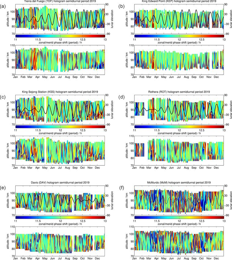
2                                                                           G. Stober et al.: SH Reynolds stress components

a residual circulation from the cold summer to the warm win-       tudes above 94 km, MF radars tend to underestimate the wind
ter pole. This important coupling mechanism is caused by           speeds, which might lead to some systematic bias in the de-
GWs carrying energy and momentum from their source re-             rived momentum flux (Wilhelm et al., 2017). Hocking (2005)
gions to the altitude of their breaking, coupling different ver-   presented a method to obtain the Reynolds stress tensor com-
tical layers in the atmosphere (Fritts and Alexander, 2003;        ponents from meteor radar observations. Based on this, sev-
Ern et al., 2011; Geller et al., 2013). The primary forcing        eral studies applied the method to optimize the data analysis
of the MLT at small scales is by gravity waves arising from        as it appeared to be challenging to get the technique imple-
various tropospheric sources, among them flow over orogra-         mented (Placke et al., 2011a, b; Andrioli et al., 2013). Fritts
phy (mountain waves), deep convection (convective gravity          et al. (2010b) and Fritts et al. (2012b) presented a momentum
waves), frontal systems, and jet stream imbalances and shear       flux meteor radar design to overcome some of the difficulties
instabilities (Fritts and Nastrom, 1992; see also the review       and evaluated the momentum flux observations using syn-
by Fritts and Alexander, 2003, and Plougonven and Zhang,           thetic data (Fritts et al., 2010a), which finally provided evi-
2014). These various GWs typically have horizontal phase           dence that these systems can be used to measure momentum
speeds comparable to the mean winds at higher altitudes;           fluxes reliably. This led to several studies using these new-
hence they are strongly influenced by varying winds along          generation systems (de Wit et al., 2014, 2016, 2017; Spargo
their plane of propagation. GWs can propagate upward un-           et al., 2019; Vierinen et al., 2019) or more powerful radars
til they become dynamical unstable or they are filtered by         such as MU radars (Riggin et al., 2016).
critical levels, where they undergo breaking and dissipation,         Climatologies of mean winds and tides are also rather
resulting in local mean flow accelerations that act as sources     sparse at the Southern Hemisphere (SH) and are essentially
of non-primary GWs.                                                affected by the vertical coupling of upward propagating grav-
   GW breaking dynamics occurs on relatively small hori-           ity waves but also provide a temporal and spatially variable
zontal scales, 10–100 km, whereas non-primary GW dynam-            background for the gravity wave propagation itself. Recent
ics occurs at larger scales, 100–300 km, and arises due to         studies with general circulation models (GCMs) have shown
the local, transient mean-flow accelerations accompanying          that mean winds are essential to understand the GW forcing
GW momentum transport (Dong et al., 2020; Fritts et al.,           (Liu, 2019; Shibuya and Sato, 2019). This is also the case for
2020). Non-primary GWs at larger scales also arise due to          tides, which provide essentially temporal variable critical fil-
interactions among larger-scale GWs in global models un-           tering for the vertical propagation of the GWs (Heale et al.,
able to resolve GW breaking dynamics (Becker and Vadas,            2020). In the past there were several studies about meso-
2018; Vadas and Fritts, 2001; Vadas and Becker, 2018). Im-         spheric winds or tides, which were often limited to a single
portantly, however, non-primary GWs accompanying GW                station or investigated only a certain tidal or wave component
breaking and interactions at lower altitudes require propaga-      (Batista et al., 2004; Fritts et al., 2010b, 2012b) and for tides
tion over large depths to become significant; hence, they play     (Beldon and Mitchell, 2010; Conte et al., 2017). Recently,
more significant roles in the lower thermosphere.                  Liu et al. (2020) used several meteor radars at the Southern
   Although GWs are such an important driver of the MLT,           Hemisphere to systematically investigate the 8 and 6 h tides
the number of observations is rather sparse. Very often the        and to obtain a more comprehensive picture of the latitudinal
GW activity is inferred by subtracting a background from           and longitudinal characteristics of these tidal modes. Further-
the wind or temperature observations to estimate potential         more, meteor radar observations have turned out to provide a
GW energy or wind variations (Ehard et al., 2015; Baum-            valuable and independent method to validate general circula-
garten et al., 2017; Chu et al., 2018; Rüfenacht et al., 2018;     tion models with data assimilation (McCormack et al., 2017)
Stober et al., 2018b; Wilhelm et al., 2019). Satellite observa-    or to investigate the inter-day variability of tidal amplitudes
tions provide an estimate of absolute momentum fluxes from         and phases (Stober et al., 2020).
the troposphere up to the mesosphere and most importantly             In this study, we present a cross-comparison of mean
a global coverage (Ern et al., 2011; Trinh et al., 2018; Hocke     winds and the diurnal and semidiurnal tide for six southern
et al., 2019). However, satellite observations are lacking the     hemispheric meteor radars located at midlatitudes and polar
directional information, and, thus, there is some ambiguity        latitudes. We present observations from 2019 and investigate
about the forcing or whether the GW momentum flux is ac-           the latitudinal and longitudinal differences of these meteoro-
celerating or decelerating the mean flow.                          logical parameters at each radar site to provide a comprehen-
   Vincent and Fritts (1987) introduced, over 2 decades ago,       sive overview and systematic analysis of the wind and tidal
a radar technique to determine the vertical flux of zonal and      and gravity wave dynamics by applying a unified diagnos-
meridional momentum utilizing medium-frequency (MF)                tic. The meteor radars are located at Tierra del Fuego (TDF),
radars using two pairs of co-planar beams. This technique          King Edward Point (KEP) on South Georgia island (Jack-
was also applied by Placke et al. (2015a, b) to determine          son et al., 2018), King Sejong Station (KSS) on King George
momentum fluxes above Andenes in northern Norway. How-             Island (Lee et al., 2018, 2016), and Rothera (ROT) Station
ever, there are only a few MF radars worldwide that are            (Sandford et al., 2010) located on the Antarctic Peninsula,
able to conduct such measurements. Furthermore, at alti-           as well as Davis Antarctic Station (DAV) (Holdsworth et al.,

Ann. Geophys., 39, 1–29, 2021                                                         https://doi.org/10.5194/angeo-39-1-2021
G. Stober et al.: SH Reynolds stress components                                                                                  3

2004) and McMurdo (McM) Antarctic Station. We discuss                A technical summary of the radars is provided in Table 1.
the presented results within the context of the stratospheric     Most of the systems have been in operation for more than
polar vortex for the year 2019. For this purpose, we comple-      a decade and have provided reliable and continuous obser-
ment our meteor radar observations with data from the Mi-         vations. Although most of these systems have been operated
crowave Limb Sounder (MLS) on board the AURA satellite            without major parameter changes, both ROT and TDF me-
(Livesey et al., 2006; Schwartz et al., 2008). Furthermore, we    teor radars have been upgraded during the observing period
utilize a recently developed retrieval algorithm, which builds    of our study. Until February 2019, the ROT system used a
on the initial momentum flux analysis formulation reported        high pulse repetition frequency (PRF) meteor mode, with
by Hocking (2005). In particular, we introduce a generalized      a PRF of 2144 Hz, a 2 km range sampling, and four coher-
approach to obtain wind variances and momentum fluxes             ent integrations. After this time, the system was upgraded
from several meteor radars (many of which are standard low        and resumed operation transmitting a 7 bit Barker code with
power systems) for the year 2019, which evolved into one of       1.5 km range sampling and a PRF of 625 Hz. We also noted
the rare minor stratospheric warming events during Septem-        a significant noise or interference at ROT before the up-
ber (Yamazaki et al., 2020). We briefly summarize how the         grade in January/February that did not allow trustworthy mo-
Reynolds stress components, also called momentum fluxes           mentum fluxes to be derived. Further, we also restricted our
and wind variances, are derived from a Reynolds decompo-          analysis of mean winds and tides to the altitude range be-
sition. The Reynolds decomposition is achieved by utilizing       tween 80–100 km. In addition, in September 2019, the TDF
an adaptive spectral filter (ASF), which allows the decompo-      transmitting scheme also changed. The original design of
sition of the meteor radar wind time series into mean winds,      the TDF transmitter (TX) configuration used eight three-
tidal components, and a GW residual (Stober et al., 2017;         element crossed Yagi antennae arranged in a circle of diam-
Baumgarten and Stober, 2019; Stober et al., 2020), similar        eter 27.6 m, each transmitting in opposite phasing of every
to the S transform used in previous studies (Stockwell et al.,    other Yagi (Janches et al., 2014). In 2019, the system trans-
1996; Fritts et al., 2010a).                                      mission strategy was upgraded with the deployment of a sin-
   The paper is structured as follows: in Sect. 2 we present      gle new TX antenna, with the goal of improving the detection
a brief introduction to the wind retrievals, the derivation of    rate of meteors at larger zenith angles for astronomical pur-
the Reynolds stress components, and the implemented mo-           poses (Janches et al., 2020). By concentrating the full power
mentum flux and GW retrieval. Section 3 contains the results      of TDF in one TX antenna, a more uniform detection pat-
of the mean flow terms, which are mean winds, diurnal and         tern is achieved that satisfies this original requirement but
semidiurnal tides, and their seasonal behavior, as well as the    also increases the number of events detected at larger zenith
determined momentum fluxes and wind variances. Our re-            angles. Finally, the McM radar is the most recent installa-
sults are discussed in Sect. 4, and the conclusions are pro-      tion, which, although it is not the most powerful radar, pro-
vided in Sect. 5.                                                 vides a very good altitude coverage. This is partly explained
                                                                  by the sporadic meteor sources and the southern location of
                                                                  the McM meteor radar. The helion, antihelion, and the south
2     Observations and methods                                    apex meteor source are above the local horizon all the time,
                                                                  contributing to the observed sporadic meteor fluxes at McM
2.1    Meteor radar observations                                  and yielding a much weaker seasonality in the altitude vari-
                                                                  ation of the meteor layer (Janches et al., 2004). In addition,
In this study, we use observations obtained with six me-          meteors arriving from these sources enter the atmosphere at
teor radars operating in the SH between 53 and 79◦ S in           fairly low entry angles (< 20◦ ; see Schult et al., 2017 for a
latitude. Four of the meteor radars can be grouped into a         Northern Hemisphere radar), leading to a much smoother ab-
cluster around the Drake Passage consisting of the Southern       lation profile of the meteoroids, and, hence, the released me-
Argentina Agile Meteor Radar (SAAMER) at Rio Grande,              teoric material is spread over a larger segment of the meteor
Tierra del Fuego, Argentina (hereafter referred to as TDF),       flight path, increasing the detectability. On the other side, the
King Sejong Station on King George Island (KSS), Rothera          orbit geometry alone does not yet provide a sufficient expla-
(ROT) on the Antarctic Peninsula, and King Edward Point           nation for the better altitude coverage at McMurdo; however,
(KEP) on South Georgia island. The other two radars are lo-       a more detailed investigation is beyond the scope of the pa-
cated almost opposite the Drake Passage at McMurdo (McM)          per.
and Davis Antarctic stations (DAV). Figure 1 shows two pan-          Several of the meteor radars used in this study employ the
els with stereographic projections of the SH, where the radar     standard meteor radar configuration of an array of five Yagi
locations are represented by red dots (left panel and Table 1).   antennas for reception, with a spacing of 2 and 2.5λ (Jacobs
The right panel in this figure shows a color contour map of       and Ralston, 1981; Jones et al., 1998). McM was set up in a
the mean elevations around each radar system to identify po-      different configuration with 1.5 and 2λ spacing due to topo-
tential orographic wave forcing sources underneath the ob-        graphic constraints. Similar to other meteor radars, most of
servation volumes.                                                them use a single Yagi antenna for transmission. Only TDF

https://doi.org/10.5194/angeo-39-1-2021                                                         Ann. Geophys., 39, 1–29, 2021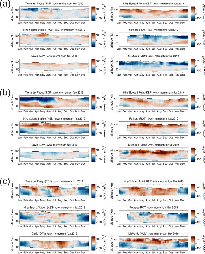
4                                                                                   G. Stober et al.: SH Reynolds stress components

Figure 1. Stereographic projection of the geographic location of the meteor radars used in this study and a map of the terrain elevation of
Antarctica, the Antarctic Peninsula, and southern Argentina to visualize the orography around each radar station. The maps are generated
using etopo1 data (Amante and Eakins, 2009).

Table 1. Technical parameters of the meteor radars.

                           TDF                KEP                KSS                ROT                DAV                McM
                           Tierra del         King Edward        King Sejong        Rothera            Davis              McMurdo
                           Fuego              Point              Station
    Freq. (MHz)            32.55              35.24              33.2               32.5               33.2               36.170
    Power (kW)             64                 6                  12                 6                  7                  30
    PRF (Hz)               625                625                440                2144/625           430                500
    Coherent               1                  1                  4                  4/1                4                  1
    integration
    Pulse code             7 bit              7 bit              4 bit              mono/              4 bit              7 bit
                           Barker             Barker             complementary      Barker             complementary      Barker
    Sampling (km)          1.5                1.5                1.8                2/1.5              1.8                1.5
    Location (lat, long)   53.7◦ S, 67.7◦ W   54.3◦ S, 35.5◦ W   62.2◦ S, 58.8◦ W   67.5◦ S, 68.0◦ W   68.6◦ S, 78.0◦ E   77.8◦ S, 166.7◦ E

employed a beam forming transmission scheme, resulting in                 gorithm presented in Stober et al. (2018a), which includes
eight main beams, as described earlier, but changed to the                the treatment of the geometry of the full Earth, based on the
use of the single crossed Yagi antenna late during the period             WGS84 rotation ellipsoid to provide more precise altitude
studied here (Janches et al., 2014, 2020). A more detailed                estimates and geodetic coordinates for each meteor, a spa-
description of the King Sejong Station meteor radar can be                tiotemporal Laplace filter, and a nonlinear error propagation,
found in Lee et al. (2018) and for the DAV meteor radar in                which is described in more detail in Gudadze et al. (2019).
Holdsworth et al. (2004).                                                 The wind retrievals are cross-validated against NAVGEM-
                                                                          HA (McCormack et al., 2017; Stober et al., 2020). The re-
2.2     Retrieval of winds and momentum flux                              sults presented in this paper are based on winds with a tem-
                                                                          poral resolution of 1 h and a vertical resolution of 2 km. The
Meteor radars have been used to measure winds in the                      minimum number of meteors per time and altitude bin for a
mesosphere–lower thermosphere (MLT) for several decades.                  successful fit is four.
Typically winds are obtained by least-squares fits, solving for              For the case of momentum fluxes, Hocking (2005) pro-
the horizontal wind velocities after binning the data into al-            posed a method using typical meteor radars, which was later
titude and time intervals (Hocking et al., 2001; Holdsworth               echoed and reformulated as correlations by Vierinen et al.
et al., 2004). In this study we retrieve winds using the al-              (2019). In this work, we present a brief derivation of the

Ann. Geophys., 39, 1–29, 2021                                                                  https://doi.org/10.5194/angeo-39-1-2021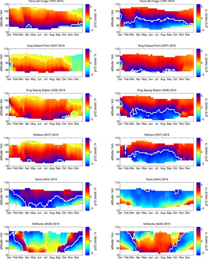
G. Stober et al.: SH Reynolds stress components 5
Reynolds stress tensor and show how the different tensor ele- Solving Eq. (7) for the unknown Reynolds stress compo-
ments are estimated from the meteor radar observations. The nents is straightforward. Typically, the terms u0 w 0 , v 0 w0 , and
starting point is the well-known radial wind equation. Each u0 v 0 are also called momentum fluxes, and the symmetric
meteor will form a trail that will be detected by the radar and Reynolds stress tensor is given by
will drift with the background wind. The radar will then de-
tect that radial velocity, via Doppler shift in the received sig- u0 2 u0 v 0 u0 w0
nal, and the three components of the background wind can be τij0 = ρui uj = ρ · u0 v 0 v 0 2 v 0 w 0 , (8)
calculated for each detected meteor using the mathematical u0 w 0 v 0 w 0 w 0 2
convention (reference to east and counterclockwise rotation):
where ρ is the atmospheric density at the altitude of the
vrad = u · cos(φ) sin(θ ) + v · sin(φ) sin(θ ) + w · cos(θ ), (1)
measurement, and the other terms in the tensor denote the
where u, v, and w are the three wind components (zonal, Reynolds stress components (wind variances and momentum
meridional, and vertical, respectively), φ is the azimuth an- fluxes), which have units of squared velocity fluctuations.
gle, θ is the off-zenith angle, and vrad is the observed ra- The Reynolds stress components are derived from the RANS
dial wind velocity. Further, it is straightforward to use the (Reynolds-averaged Navier–Stokes) equations, assuming an
standard Reynolds decomposition of the wind, separating the incompressible Newtonian fluid and that the Reynolds aver-
wind components into a mean flow (u, v, w) and wind fluc- age of the fluctuations vanishes (u0 = 0), which requires the
tuations (u0 , v 0 , w0 ): averaging to be long enough to cover the inertia GW periods
u= u + u0 of several hours or longer. The spatial scales can theoreti-
cally be estimated by selecting different volumes inside the
v= v + v0
domain area; however, practically the meteor statistics is of-
w= w + w0 . (2) ten not sufficient to get reliable results.
As we are mainly interested in the momentum flux associated However, there are some caveats of the theory outlined
with GWs, the mean flow terms containing the background above, when it comes to implementing the algorithm and ac-
wind and the diurnal and semidiurnal tide have to be sub- tually applying it to meteor radar observations. One difficulty
tracted/removed from the observed radial velocities for each is the Reynolds decomposition into the mean flow and the
meteor. Thus, we model the mean flow radial velocity by GW fluctuations. Previous studies often limited the analy-
sis to a narrower angular region (Fritts et al., 2010a; Placke
vradm = u · cos(φ) sin(θ ) + v · sin(φ) sin(θ ) + w · cos(θ ). (3) et al., 2015a) using only off-zenith angles between 10–50◦ ,
0 ), which now only con-
The radial velocity fluctuations (vrad reducing significantly the number of meteors for the analysis
tain GW contributions, are obtained by subtracting the mean per time and altitude bin, which in turn required longer av-
flow radial velocity (vradm ) from the observed radial velocity eraging or was achieved by an active beam forming antenna.
(vrad ) measurements: Such an antenna directed more energy towards an angular re-
0 gion as for TDF (Fritts et al., 2010b, a) or the meteor radar
vrad = vrad − vradm . (4)
at Trondheim (de Wit et al., 2014). The process by which
Furthermore, the GW fluctuations can be modeled by this much stricter angular selection of meteors improved the
0
vradm = u0 ·cos(φ) sin(θ )+v 0 ·sin(φ) sin(θ )+w0 ·cos(θ ). (5) momentum flux estimates was the reduction of projection er-
rors due to the Earth’s ellipsoid shape, which caused apparent
Considering that these radial velocity fluctuations are mostly and arbitrary contributions to the fluctuation terms. Stober
driven by GW, the Reynolds stresses can be computed by et al. (2018a) proposed to minimize this type of uncertainty
minimizing the following quantity (Hocking, 2005): by computing each meteor’s geodetic position relative to the
X 2 2 WGS84 reference ellipsoid, which improves the altitude de-
0
2 0
3= vrad − vradm . (6) termination but also reduces projection errors for the azimuth
and off-zenith angle. The benefit of this full Earth geometry
Inserting Eq. (5) into Eq. (6) leads to the well-know momen- correction is that there is no longer a need to reduce the an-
tum flux terms: gular region, and all meteors up to off-zenith angles of 65◦
X 2 0 2 can be used for the analysis. Typical specular meteor radars
3= 0
vrad − u · cos(φ)2 sin(θ )2 (single Yagi antenna on transmission) detect most meteors
2 2
at off-zenith angles between 50 and 70◦ . However, meteors
+ v 0 · sin(φ)2 sin(θ )2 + w0 · cos(θ )2 at larger zenith angles are further away from the radar and,
+ 2u0 v 0 · cos(φ) sin(φ) sin(θ )2 thus, are more prone to altitude errors. The typical angular
precision of the employed receiver arrays is approximately
+ 2u0 w 0 · cos(φ) sin(θ ) cos(θ )
1.5–1.7◦ (Jones et al., 1998). A limit of 65◦ presents a more
2 optimal choice to maximize the number of meteors entering
0 0
+ 2v w · sin(φ) sin(θ ) cos(θ ) . (7)
the analysis while keeping a sufficient altitude precision.
https://doi.org/10.5194/angeo-39-1-2021 Ann. Geophys., 39, 1–29, 2021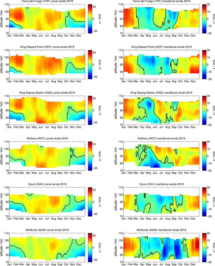
6                                                                            G. Stober et al.: SH Reynolds stress components

   Another important aspect related to the momentum flux es-       u0 2 , v 0 2 , and w0 2 , respectively. Such negative values were re-
timation is the proper removal of the background flow, which       ported in Placke et al. (2011a), but this appears to be a minor
was already outlined by Fritts et al. (2010a), Placke et al.       issue in our retrievals. Only a negligible number of fits re-
(2011b), and Andrioli et al. (2013) and later confirmed by         sulted in negative values for just some of the radar systems
de Wit et al. (2014). In particular, tides have large ampli-       utilized in this work.
tudes in the MLT, causing large vertical and temporal shears           In addition, we performed some test retrievals to account
within a time and altitude bin. Noting that Hocking (2005)         for the vertical velocity bias intrinsic to the meteor radar
and Placke et al. (2011b) suggested the use of at least 30         observations. Specular meteors have trail lengths of up to
meteors for a successful momentum flux fit, which is often         several kilometers where the radio waves are scattered, and,
achieved by temporal averaging, the importance of the tem-         thus, meteors entering the Earth’s atmosphere at steep en-
poral shear becomes evident.                                       try angles can encounter strong vertical wind shears, which
   In this study we use the adaptive spectral filter (ASF)         lead to a rotation of the trail, causing systematic errors. In
to perform the Reynolds decomposition to characterize the          particular, during the local summer months, this can lead to
background flow and the GW fluctuations. A first version           a systematic deviation of a few centimeters per second for
of the ASF(1D) (temporal domain) was presented in Stober           midlatitude stations.
et al. (2017). Here we make use of the ASF(2D), which em-              Very often wind fits are performed by assuming w =
ploys a vertical regularization constraint for the mean wind       0 m s−1 (Hocking et al., 2001; Holdsworth et al., 2004).
and tides, assuming a smooth vertical phase progression for        However, here we use the retrievals as presented in Stober
each wave without an explicit vertical wavelength thresh-          et al. (2018a), who used the vertical wind velocity as quality
old (Pokhotelov et al., 2018; Baumgarten and Stober, 2019;         control. Typically, we obtain daily mean values of the order
Wilhelm et al., 2019). The ASF accounts for the continu-           of ±0.25 m s−1 , which is more than an order of magnitude
ous variation of the mean flow as well as for the intermit-        less than reported by Egito et al. (2016). However, the re-
tent behavior of the tides. Thus, we obtain hourly resolved        maining bias due the vertical winds, which potentially has the
background wind fields for each altitude and time bin for          wrong sign, had no impact on the retrieved Reynolds stresses.
the zonal, meridional, and vertical wind component, respec-            Finally, in order to get confidence in the retrievals, we per-
tively. This background wind field contains the mean flow          formed several test cases similar to the ones presented in
and the diurnal, semidiurnal, and terdiurnal tidal component.      Fritts et al. (2010a). Therefore, we extracted the observed
However, the terdiurnal tide usually has a much smaller am-        meteor detections from TDF and synthesized wind fields
plitude (Liu et al., 2020) compared to the diurnal and semid-      including altitude-dependent mean winds and tides with a
iurnal tides and, thus, is not discussed here further. Further-    vertical wavelength of 80 km and various altitude-dependent
more, we perform a linear interpolation of the background          GW fields to optimize the retrieval setting with respect to
wind field to the actual occurrence time and altitude for each     the regularization strength, the required statistics, and the ap-
meteor to estimate the vradm term, minimizing any contribu-        plied averaging. Performing these tests, we find minor de-
tion from the background flow. This procedure is effective in      viations from the synthetic wind and GW fields only at the
mitigating possible contamination due to tides and permits         upper and lower edges of the meteor layer. The tidal ampli-
the use of a much longer averaging window. In this study           tudes were retrieved within ±2 m s−1 compared to the syn-
we use 64 h and a minimum of 100 meteors to determine the          thetic data. The momentum fluxes agreed for the 30 d median
Reynolds stress components. However, for the seasonal cli-         remarkably well. We also tested the possibility to retrieve the
matology, only solutions with more than 1000 meteors enter         vertical wind fluctuation amplitudes and found mean devia-
the statistics.                                                    tions of ±0.01 m s−1 residual bias for the synthetic fields and
   The algorithm is implemented similar to that performed          about ±0.25 m s−1 bias in our observations.
for wind retrievals in Stober et al. (2018a). The first guess
is provided by a classical least-squares fit. Based on this ini-   2.3   MLS satellite observations
tial iteration, we compute the spatiotemporal Laplace filter,
which provides a predictor for each time and altitude bin.         To bring the local radar observations into the global con-
This predictor enters all further iterations as regularization     text we calculate the geostrophic zonal wind as described
(Tikhonov) and is updated each time. The spatiotemporal            in Matthias and Ern (2018) from geopotential height (GPH)
Laplace filter turns out to be beneficial for ill-conditioned      data from the Microwave Limb Sounder (MLS) on board the
problems due to the random occurrence of meteor detections         Aura satellite (Waters et al., 2006; Livesey et al., 2015). MLS
and asymmetries in the spatial sampling; these can result in       has a global coverage from 82◦ S to 82◦ N on each orbit and
difficulties in determining all parameters with similar quality.   a usable height range from approximately 11 to 97 km (261–
   Furthermore, we perform a nonlinear error propagation           0.001 hPa), with a vertical resolution of ∼ 4 km in the strato-
similar to the one presented in Gudadze et al. (2019). The         sphere and ∼ 14 km at the mesopause. The temporal resolu-
statistical uncertainties are updated in each iteration step. We   tion is 1 d at each location, and data are available from Au-
also tested barrier functions to penalize negative values of       gust 2004 until the present (Livesey et al., 2015). Version 4

Ann. Geophys., 39, 1–29, 2021                                                          https://doi.org/10.5194/angeo-39-1-2021
G. Stober et al.: SH Reynolds stress components                                                                                7

MLS data were used in this paper, along with the applica-        cant asymmetry in the southern hemispheric wind systems.
tion of the most recent recommended quality screening pro-       As expected, looking at the general morphology, the seasonal
cedures from Livesey et al. (2015). For our analyses the orig-   zonal wind pattern for 2019 is remarkably similar between
inal orbital MLS data are accumulated in grid boxes with 10◦     both locations. There are only marginal differences in the
grid spacing in longitude and 5◦ in latitude. Afterwards they    zonal magnitudes considering the overall agreement of the
are averaged at every grid box and for every day, generally      zonal wind structures. This is also the case for the meridional
resulting in a global grid with values at every grid point.      winds during the summer months (DJF). However, during
                                                                 the winter season, the meridional wind structure is signif-
                                                                 icantly different between both stations. The morphology at
3     Results                                                    DAV appears to be less asymmetric, with a tendency to show
                                                                 increased southward wind magnitudes towards the end of the
3.1    Mean winds 2019                                           winter season, whereas at ROT the highest southward winds
                                                                 are recorded at the begin of the winter season 2019.
As pointed out in the previous section, we perform a                The southernmost location in our analysis is McM at
Reynolds decomposition in order to separate a mean flow          78◦ S. The seasonal zonal wind morphology compares well
from the GW fluctuations. Thus, we analyze the data with         with that measured at DAV and ROT but shows much weaker
the adaptive spectral filter (ASF) technique (Baumgarten and     wind magnitudes. Similar to observations in the Northern
Stober, 2019) to obtain daily mean winds, as well as diurnal     Hemisphere, the summer zonal wind reversal altitude also in-
and semidiurnal tides.                                           creases with increasing southern latitude. Compared to DAV,
   We first compare the seasonal zonal and meridional winds      the meridional winds are intensified during the summer and
of all six locations to identify any seasonal and local dif-     winter seasons. Furthermore, the asymmetry during the win-
ferences. Figure 2 shows the seasonal zonal and meridional       ter months is also present at McM, which shows, similarly
wind pattern during 2019 obtained from the daily mean zonal      to DAV, the highest southward meridional winds towards
and meridional winds after applying a 30 d running median        the end of the winter season as a double structure. In fact,
shifted by 1 d. This reveals any seasonal variability by re-     the southward meridional winds at McM during July and
moving atmospheric waves with shorter periods. A similar         September 2019 are the strongest of all locations.
analysis was applied in Wilhelm et al. (2019) for meteor
radars in the Northern Hemisphere in order to derive mean
                                                                 3.2   Diurnal tidal amplitudes and phases measured
wind climatologies. Significant differences between the lo-
                                                                       during 2019
cations can be observed from this figure, in particular during
the SH winter seasons (JJA). Both TDF and KEP observa-
tions, operated at almost the same latitude at 54◦ S, show a     Atmospheric tides provide a time-variable background fil-
similar morphology for the zonal winds, and only the merid-      ter for the vertical propagation of GWs, which can, depend-
ional winds deviate from each other during June and July.        ing on the tidal phase and the propagation direction of the
At the tip of South America, TDF shows that the meridional       GW, lead to GW breaking and dissipation. These break-
winds experience a sign reversal around June/July, which is      ing events might trigger/foster the generation of secondary
not present over KEP. The meridional winds also seem to          or non-primary waves (Heale et al., 2020). Thus, tides are
have a semiannual oscillation at both locations.                 essentially contributing to the Reynolds decomposition. In
   Further polewards at KSS and ROT (62 and 67◦ S, respec-       particular, the day-to-day variability is crucial for the mo-
tively), which are at a similar longitude as TDF, the zonal      mentum flux analysis. Typically, atmospheric tides are de-
winds reflect a similar seasonal behavior compared to KEP        rived assuming phase stability over a certain period of time,
and TDF but with a slightly weaker wind magnitude. How-          which can be several days, weeks, or months (Murphy et al.,
ever, the meridional winds are fairly consistent during the      2006; Hoffmann et al., 2010; Conte et al., 2017; He et al.,
summer months compared to the midlatitude radars but de-         2018; Pancheva et al., 2020). More recent studies favor much
viate considerably during the winter season. There is even       shorter windows of 24 to 48 h to account for the intermit-
a noticeable difference between KSS and ROT, even though         tent behavior of tides (Stober et al., 2017; Wu et al., 2019;
the systems are located rather close together. At ROT and        de Araújo et al., 2020; Das et al., 2020), in particular, phases
KSS the meridional winds only show a typical winter behav-       of atmospheric tides that appear not to be constant with time
ior during April, May, and June and approximately north-         (Ward et al., 2010; Baumgarten and Stober, 2019; Stober
ward winds for the other months above 80–85 km. Only dur-        et al., 2020). In this study, all tidal amplitudes and phases
ing September and at altitudes above 90 km above KSS does        were determined with the ASF, which, similar to wavelet
a short southward wind patch occur.                              spectra, adapts the window length to the period of the fitted
   Comparing the observed wind fields measured at ROT and        frequencies. The obtained daily tidal amplitudes are vector-
DAV, which are only separated by 2◦ in latitude but by 170◦      averaged using 30 d medians centered at the respective day
in longitude, further emphasizes the existence of a signifi-     to derive the seasonal variation.

https://doi.org/10.5194/angeo-39-1-2021                                                        Ann. Geophys., 39, 1–29, 2021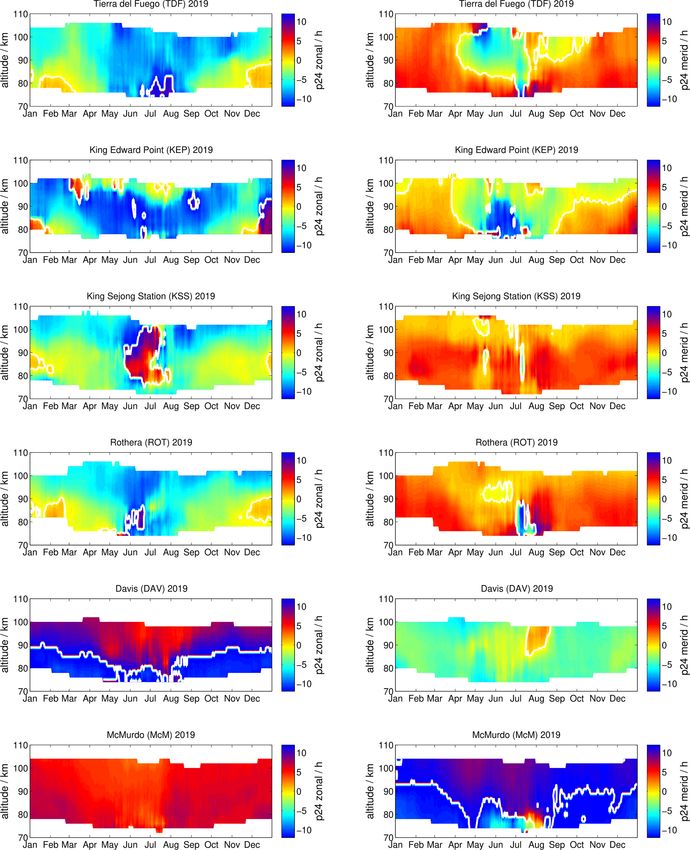
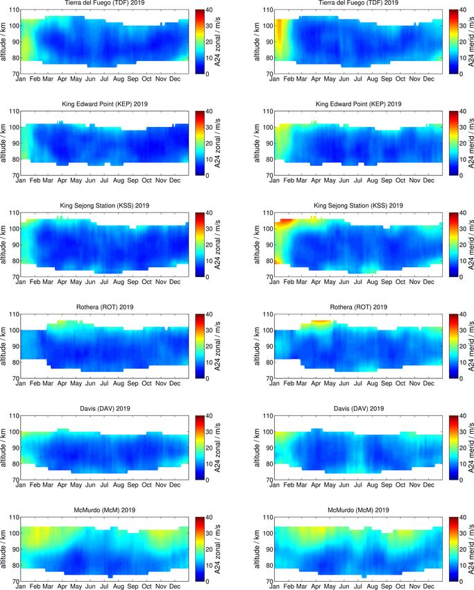
8                                                                               G. Stober et al.: SH Reynolds stress components

Figure 2. Comparison of zonal and meridional mean winds for each station during the year 2019. The left column shows the zonal component
and the right column the meridional wind. All stations are sorted according to their latitude from TDF, KEP, KSS, ROT, and DAV to McM.

   Figure 3 presents the seasonal variation of the diurnal            100 km the diurnal tide remained of significant magnitude
tidal amplitudes measured at each station. Although the daily         until May 2019. Evidently, for the other months the diurnal
mean winds showed significant differences between TDF,                tidal amplitudes remained fairly weak (< 10 m s−1 ) at alti-
KEP, KSS, and ROT, the seasonal behavior of the diurnal               tudes between 80–100 km during 2019. KSS and ROT indi-
tide is rather consistent between all four locations. There           cate a small diurnal tidal enhancement for July/August and in
is a pronounced summer maximum in the zonal and merid-                December below 80 km and above 100 km altitude. The De-
ional amplitudes from January to February at altitudes from           cember enhancements are also found at TDF but almost dis-
78–106 km. The meridional tidal amplitudes tend to exceed             appear at KEP. DAV measurements show basically the same
the zonal amplitude by up to 10 m s−1 . At altitudes above            seasonal diurnal tide behavior but with weaker amplitudes.

Ann. Geophys., 39, 1–29, 2021                                                             https://doi.org/10.5194/angeo-39-1-2021
G. Stober et al.: SH Reynolds stress components                                                                              9

Figure 3. Same as Fig. 2 but for the diurnal tidal amplitudes.

The winter diurnal tidal enhancement in June/July appears        minimum, whereas the meridional component shows a tidal
to be more pronounced. However, the southernmost meteor          enhancement.
radar at McM observes a significantly different seasonal di-        Diurnal tidal phases are shown in Fig. 4. The tidal phases
urnal tidal pattern. The summer maximum is much more pro-        are given in UTC; hence, longitudinal differences are present
nounced compared to the other stations and shows ampli-          as phase shifts. As expected the diurnal phases are much
tudes of 20 m s−1 from January to April at 90 km and above       more variable during time with low tidal amplitudes for TDF,
and again from October to December. There is also a notice-      KEP, KSS, and ROT. During the summer months of January
able difference between the zonal and the meridional diur-       and February 2019, the diurnal phases are more stable and
nal tidal amplitude. The zonal component indicates a winter      indicate rather long vertical wavelengths but with significant

https://doi.org/10.5194/angeo-39-1-2021                                                       Ann. Geophys., 39, 1–29, 2021
10                                                                         G. Stober et al.: SH Reynolds stress components

Figure 4. Same as Fig. 2 but for the diurnal tidal phases.

differences between the zonal and the meridional compo-           3.3   Semidiurnal tidal amplitudes and phases measured
nents. However, the phase plots indicate a distinct seasonal            during 2019
pattern, showing phase drifts of several hours at the same al-
titude over the course of the year. The further south the loca-
tion of a meteor radar is, the less characteristic the seasonal   At midlatitudes and high latitudes, semidiurnal tides are the
behavior is. Measurements at DAV and McM indicate a de-           dominating tidal wave during the course of the year (Ha-
creased variability of the diurnal tidal phases throughout the    gan and Forbes, 2002, 2003). Figure 5 shows the vector-
year. At DAV there are periods suggesting almost phase sta-       averaged semidiurnal tidal amplitudes measured by all six
bility over several weeks, instead of the typical continuous      meteor radars using again a 30 d median shifted by 1 d in
variation reflected by the other stations.                        analogy to the mean winds and diurnal tides.

Ann. Geophys., 39, 1–29, 2021                                                       https://doi.org/10.5194/angeo-39-1-2021
G. Stober et al.: SH Reynolds stress components                                                                               11

Figure 5. Same as Fig. 2 but for the semidiurnal tidal amplitudes.

   The seasonal structure of the semidiurnal tide reveals a          the tidal amplitudes show a decrease with increasing polar
rather interesting pattern for the SH. Semidiurnal tides mea-        latitude, which is also observed at the Northern Hemisphere.
sured at TDF, KEP, KSS, and ROT show some similarities for           However, the meridional semidiurnal tide shows a clear lon-
the zonal component, resulting in amplitudes with values be-         gitude dependence and asymmetry compared to the zonal
low < 10 m s−1 during the summer months January to mid-              tidal amplitudes, which was not reported previously (Conte
March. From April to June, all four stations show a strong           et al., 2017). At the longitude of TDF and ROT the merid-
semidiurnal tidal activity, with amplitudes up to 40 m s−1 , an-     ional tidal component is much weaker during April to June
other minimum of the tidal activity in July, and a secondary         compared to the zonal. At KSS, which is further east, sim-
maximum from August to the end of the year. Furthermore,             ilar amplitudes for the zonal and meridional component are

https://doi.org/10.5194/angeo-39-1-2021                                                          Ann. Geophys., 39, 1–29, 2021
12                                                                        G. Stober et al.: SH Reynolds stress components

Figure 6. Same as Fig. 2 but for the semidiurnal tidal phases.

observed. This was also found at KSS in a previous study            The semidiurnal tidal seasonal behavior observed at DAV
reporting the tidal amplitudes under solar maximum condi-        looks quite different from the stations that are located further
tions, which resulted in larger amplitudes of the semidiurnal    to the north. The amplitudes are much weaker and barely
tide (Lee et al., 2013). KEP, which is 25◦ eastward, shows       reach values of 25 m s−1 , and there are four periods during
the opposite behavior, and the meridional component of the       which an increased activity is observed, which are during
semidiurnal tide reaches the highest amplitudes in April to      January–February, May, August–September, and December.
June. Such differences with longitude might be related to the    The largest tidal amplitudes are observed during May 2019.
superposition of migrating and non-migrating tides (Murphy          Further to the south, at McM station, the semidiurnal tide
et al., 2006).                                                   exhibits only a very faint seasonal structure. Most of the
                                                                 time the amplitudes are below 10 m s−1 . Only during March,

Ann. Geophys., 39, 1–29, 2021                                                       https://doi.org/10.5194/angeo-39-1-2021
G. Stober et al.: SH Reynolds stress components 13
Figure 7. Comparison of semidiurnal tidal vertical wavelengths of (a) TDF, (b) KEP, (c) KSS, (d) ROT, (e) DAV, and (f) McM.
May, and November–December and below 90 km altitude are Semidiurnal tidal phases are displayed in Fig. 6, where
there periods where amplitudes exceed 10 m s−1 . This is sur- it can be seen that the semidiurnal tidal phases reflect sim-
prising when we compare these values with measurements ilar features than those present in the amplitudes. TDF, KEP,
performed at geographically conjugate Northern Hemisphere KSS, and ROT show a very similar seasonal structure, in-
latitude. For instance, at Svalbard (78.17◦ N, 15.99◦ E), the dicating continuous changes of the tidal phases through-
semidiurnal tide still reflects a similar seasonal activity to out 2019 at all altitudes. At DAV and McM, on the other
other polar and midlatitude locations (Wilhelm et al., 2019; hand, the observed phases indicate an even more pronounced
Pancheva et al., 2020). This is obviously not the case in the seasonal structure and faster gradual phase drifts. In partic-
SH and represents a remarkable interhemispheric difference. ular, at McM the phases appear to be more variable, which
is likely due to the generally weaker amplitudes, pointing to-
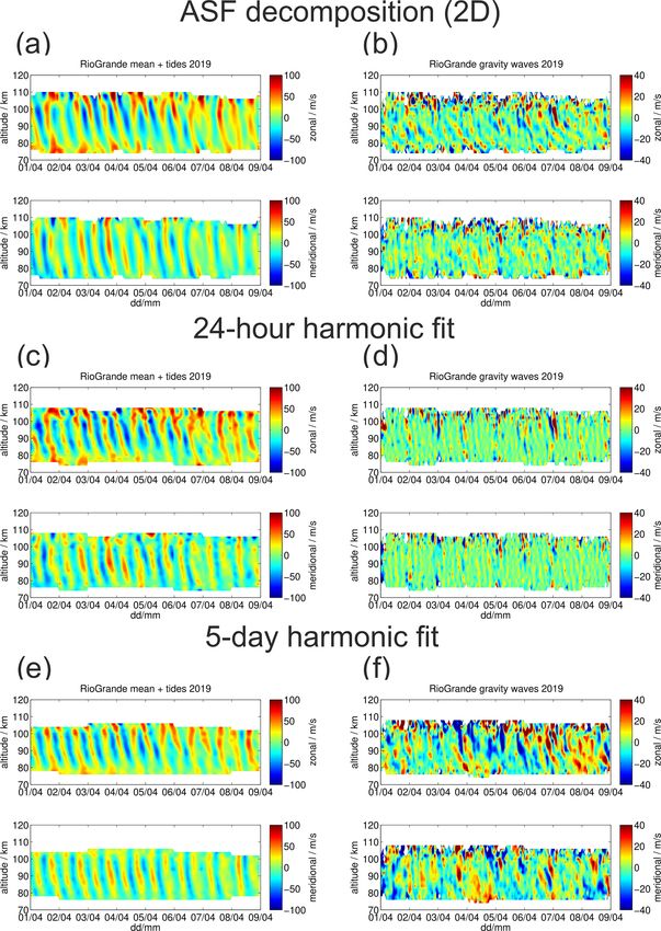
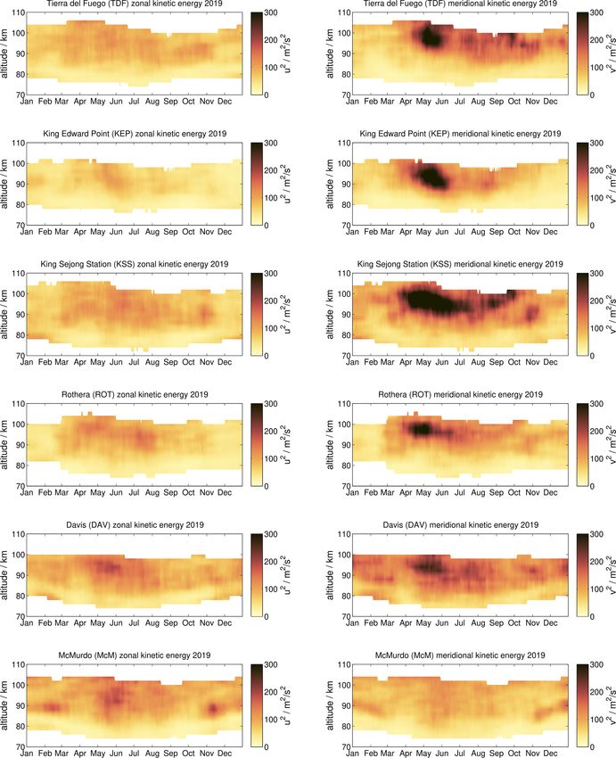
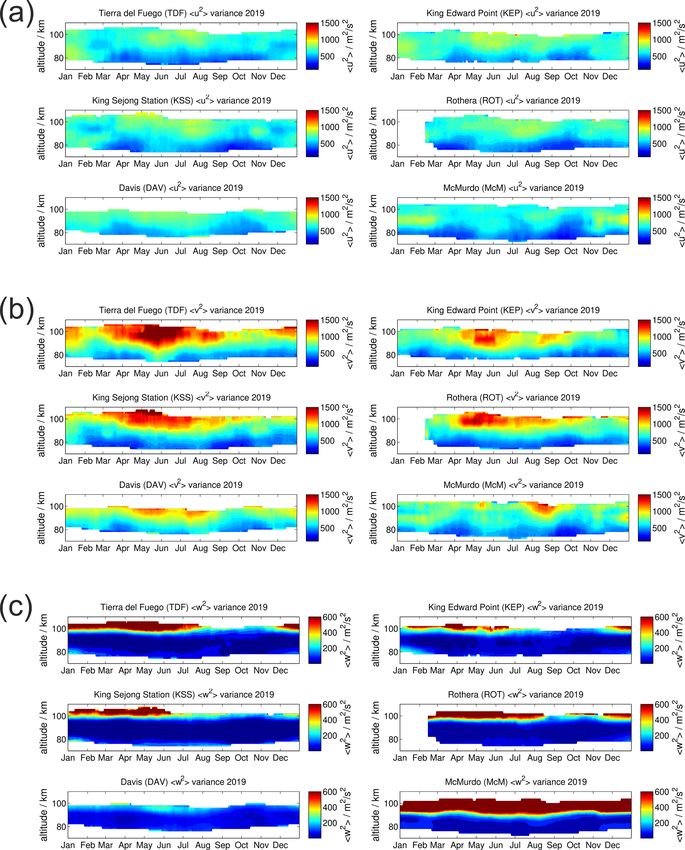
https://doi.org/10.5194/angeo-39-1-2021 Ann. Geophys., 39, 1–29, 202114 G. Stober et al.: SH Reynolds stress components wards a much weaker and more intermittent excitation of the to identify potential changes in the Hough modes of the tide, tides. which are solutions of the Laplace tidal differential equation Comparing the seasonal phase behavior of the SH to that (Lindzen and Chapman, 1969; Wang et al., 2016). The ver- measured at conjugate latitudes in the Northern Hemisphere tical wavelengths show a similar latitude and longitude de- indicates that there are some differences. In the Northern pendence as already discussed for the semidiurnal tidal am- Hemisphere, from midlatitudes to high latitudes, the semid- plitudes and phases. The observations at TDF, KEP, KSS, iurnal tides show a seasonal asymmetry between the win- and ROT indicate almost the same vertical wavelengths from ter to summer transition and the fall transition (Portnyagin March to October 2019 of about 70–100 km. This corre- et al., 2004; Wilhelm et al., 2019; Stober et al., 2020). The sponds to the time with the largest semidiurnal tidal am- fall transition is accompanied by a significant phase change plitudes. However, the seasonal summer months January– from September to November, whereas in the SH this feature February and November–December show a longitudinal dif- is very weak at TDF and ROT (March to May) and almost ference. KEP and KSS observe much longer vertical wave- negligible for KEP and KSS. lengths of up to 1000 km during these months, compared Finally, we briefly discuss the presence of a potential lu- to the stations located to the west. These very long vertical nar tide. Sandford et al. (2006, 2007) estimated the lunar wavelengths are associated with times with a small semidi- tide amplitude from two northern hemispheric meteor radars urnal tidal amplitude. The results obtained at DAV reflect a and Davis MF radar in the SH and found values of 1– slightly different seasonal behavior. There, the longest verti- 2 m s−1 , which is negligible compared to the typical GW am- cal wavelengths are observed in March–April, followed by a plitudes of about 20–30 m s−1 for the resolved waves. How- stable hemispheric winter season until August, and a grad- ever, Forbes and Zhang (2012) investigated a potential lunar ual decreasing of vertical wavelengths towards the end of tide amplification due to the Pekeris resonance. They found the year. The results at McM show an even more compli- favorable conditions to shift the Pekeris peak towards the lu- cated picture due to the almost vanishing semidiurnal tidal nar tide periods M2 (12.42 h) and N2 (12.66 h), during the amplitudes. Only during the local summer months of Jan- time of major sudden stratospheric warming in 2009 in the uary/February and November/December are meaningful ver- Northern Hemisphere, as only during the time of the wind re- tical wavelengths derivable, with vertical wavelengths of versal do the vertical temperature and wind structure satisfy about 70–100 km. It is also worth mentioning that the agree- the resonance conditions. Later, Zhang and Forbes (2014) ar- ment between the zonal and meridional wavelengths is re- gued that the Pekeris resonance peak is rather broad, and, markable and provides further confidence in the applied ASF thus, more or less each sudden stratospheric warming can technique used for the Reynolds decomposition. cause a lunar tide amplification. These reports triggered several studies investigating the lu- 3.4 Reynolds stress components nar tide and its relevance for mesosphere dynamics. How- ever, most of the observational diagnostics (wavelet or har- Gravity waves are an essential driver of the MLT dynamics monic fitting) separating the lunar tide from the semidiurnal and variability, carrying energy and momentum from their tide applied long windows of 21 d or even longer periods up source region to the altitude of their deposition. The break- to several months, assuming phase stability of the semidiur- ing of GWs can trigger the generation of non-primary GWs, nal tide (Forbes and Zhang, 2012; Chau et al., 2015; Conte which again can propagate upwards (Becker and Vadas, et al., 2017; He et al., 2018; Siddiqui et al., 2018). How- 2018; Vadas and Becker, 2018), causing a complex interac- ever, as shown in Fig. 6, the semidiurnal tidal phase shows tion chain for the GW activity and the resulting forcing at considerable variability and seasonal changes, and, thus, the the MLT. The acceleration and deceleration of the mean flow assumption of phase stability for the semidiurnal tide is not due to momentum and energy transfer by breaking GW can valid. Therefore, we performed a holographic analysis to test be estimated from the vertical gradient of the gravity wave whether a temporally variable semidiurnal tidal phase could momentum flux (Ern et al., 2011). be misinterpreted as a lunar tide (see Appendix A1) (Sto- From our Reynolds decomposition and the retrieval, we ber et al., 2020) . In fact, the holograms often exhibit a shift determine three momentum fluxes, which are often referred towards the M2 frequency (12.42 h) uncorrelated with the lu- to as the vertical flux of zonal momentum < uw >, the verti- nar orbit. Given these results, and considering that there was cal flux of meridional momentum < vw >, and the horizon- only a minor stratospheric warming in September 2019 (Ya- tal momentum flux < uv >, where the denotes temporal mazaki et al., 2020), we consider the lunar tide to be a minor averaging. wave with a negligible amplitude compared to GWs, and we Figure 8 shows all three momentum flux components as did not make an attempt to remove this tidal component in a 30 d median shifted by 1 d for the year 2019. There are our Reynolds decomposition. three groups of panels presenting the vertical flux of zonal For the sake of completeness, we also estimated the verti- momentum (panel a), the vertical flux of meridional momen- cal wavelengths of the semidiurnal tide, which is presented tum (panel b), and the horizontal momentum flux (panel c). in Fig. 7. The vertical wavelength provides a good overview The stations are sorted according to their latitude within each Ann. Geophys., 39, 1–29, 2021 https://doi.org/10.5194/angeo-39-1-2021
G. Stober et al.: SH Reynolds stress components                                                                                  15

Figure 8. Comparison of vertical flux of zonal and meridional momentum and horizontal momentum flux for each station during the year
2019 for (a) the zonal momentum flux, (b) the meridional momentum flux, and (c) the horizontal momentum flux.

panel to allow for an easier comparison between the sites.             The vertical flux of zonal momentum < uw > is rather
The results shown in this figure indicate that, for all six me-     variable with longitude and latitude. Observations at TDF
teor radar observations, there is a characteristic seasonal pat-    and ROT show some similarities regarding the seasonal
tern, with noticeable differences between the different loca-       structure. During the local summer, both indicate positive
tions.                                                              zonal momentum fluxes at the altitude of the zonal wind re-
                                                                    versal. At higher altitudes, above 95–100 km, the zonal mo-

https://doi.org/10.5194/angeo-39-1-2021                                                           Ann. Geophys., 39, 1–29, 2021
16 G. Stober et al.: SH Reynolds stress components Figure 9. Same as Fig. 8 but for the (a) zonal, (b) meridional, and (c) vertical wind variances. mentum flux reverses to negative values. The winter season KSS a variable zonal momentum flux is measured that seems appears to be more variable, which might be related to the to be in better agreement with TDF and ROT results. Further minor warming in September 2019 and the wave activity be- to the south, at DAV and McM, the seasonal behavior of the fore. To the east, at KEP and KSS, positive zonal momen- zonal momentum flux seems to reflect the features that are tum fluxes at the higher altitudes (95–105 km) are observed already found at KEP but with different magnitudes. throughout the year but a rather different behavior during the The vertical flux of meridional momentum presented in local winter season at the altitudes below. In particular, at Fig. 8 exhibits some longitudinal dependence. Observations Ann. Geophys., 39, 1–29, 2021 https://doi.org/10.5194/angeo-39-1-2021
G. Stober et al.: SH Reynolds stress components                                                                                  17

at TDF and KEP show approximately the opposite verti-               the resolved GWs with periods longer than 2 h and horizon-
cal structure of the meridional momentum flux, pointing out         tal wavelengths of more than 300 km, whereas the wind vari-
that the meridional drag (acceleration and deceleration) re-        ances obtained using Hocking (2005) include the GW vari-
verses between their longitudes. Furthermore, results from          ances from all temporal and spatial scales. The GW variances
KEP, KSS, and ROT show a good agreement of the vertical             from the residuals are shown in Fig. A2 in the Appendix.
structure and seasonality of the meridional momentum flux
throughout the year. Measurements at DAV still show some
features of the seasonal meridional momentum flux behav-            4   Discussion
ior but with decreasing magnitude, while at McM, the results
show once again a seasonal dependency comparable to that            Meteor radar observations of GW momentum fluxes have
obtained at KEP.                                                    now been performed for more than a decade (Hocking, 2005;
   Only the horizontal momentum flux < uv > shows a sim-            Fritts et al., 2010a; Placke et al., 2011b; Andrioli et al.,
ilar seasonal behavior at TDF, KEP, KSS, ROT, and DAV,              2013; de Wit et al., 2014, 2017). However, the results were
with negative values of −50 m2 s−2 during the seasonal sum-         not always conclusive and often difficult to interpret. Many
mer and positive values in winter from April to October. The        of these former studies focus on understanding the method
local winter shows more variability and a semiannual struc-         and how to optimize the analysis procedure (Fritts et al.,
ture at some sites, similar to the mean zonal and meridional        2010a, 2012b; Placke et al., 2011b; Andrioli et al., 2013;
winds. At McM this seasonal variation is still visible but with     Placke et al., 2015a). Although the Reynolds decomposition
a much weaker magnitude.                                            appears to be straightforward, it can be challenging to do
   The seasonally dependent Reynolds stress components on           a proper and robust implementation and successfully sepa-
the main diagonal of the tensor are also investigated. These        rate the mean flow from the GW fluctuations. Fourier-based
terms are also often called zonal, meridional, and vertical         methods often require long averaging windows in order to
wind variances. Figure 9 shows all three variances for each         get a proper resolution but do not capture the intermittency
station. Note that the color scale for the vertical variances is    of the background sufficiently (see Fig. A3). For shorter win-
5 times smaller compared to the horizontal wind fluctuations.       dows the irregular sampling of meteors in time and altitude
The zonal and meridional variances exhibit a seasonal struc-        again causes deviations from a regular grid, and, addition-
ture and a rather obvious altitude dependence. The highest          ally, data gaps have to be considered when applying wavelet
variances are observed at the highest altitudes, which is ex-       or Fourier techniques. Another complication of the meteor
pected, considering that the Reynolds stresses are weighted         radar momentum fluxes is that there are no “ground truth
by the atmospheric density, which decreases exponentially           data” available to validate the measurements. Satellite ob-
with altitude. It is also a common feature for all sites that the   servations provide only a total GW momentum flux without
meridional velocity variances exceed the zonal fluctuations.        directional information obtained from temperature fluctua-
The seasonal behavior of the zonal and meridional variances         tions after removing atmospheric tides up to wave number 4,
at all stations reflects a semi-annual variation, showing min-      assuming a stationary phase behavior over a couple of days
imum variances during the equinoxes, when the mean winds            (Ern et al., 2011; Trinh et al., 2018), and thus confidence in
are smallest at altitudes below 95–100 km. Above 100 km the         the methodology relies on tests with synthetic fields such as
seasonal characteristic appears to be less pronounced. The          those presented in Fritts et al. (2010a, 2012a).
vertical wind variances are the most challenging values to re-         As we are mainly interested in the GW momentum flux
trieve. Their seasonal behavior is less obvious. However, the       and wind variances, we have to evaluate the presence of po-
vertical wind variances also indicate increasing values with        tential error sources in the Reynolds decomposition method-
decreasing density. Results at McM are exceptional in this          ology carefully. In particular, atmospheric tides show a very
respect, and the vertical wind variances exceed the values          intermittent behavior of the amplitude and phase, which
that are derived at all other stations. At present we can only      causes some issues in the decomposition when long win-
speculate on the source of these large values. A possibility is     dows (several days/weeks or months) are used. Thus, we per-
that McM lies underneath the auroral oval, and, thus, the al-       formed some tests to optimize the mean flow and tidal and
titudes above 90 km are strongly influenced by precipitating        GW decomposition, applying the ASF, a 1 d harmonic fit,
particles and associated effects like Joule heating that might      and a 5 d harmonic fit (see Appendix A3). The comparison
trigger stronger vertical variations (Fong et al., 2014).           indicates that the Reynolds decomposition tends to be very
   To gain confidence in our retrieved horizontal wind vari-        sensitive to the applied technique, impacting the tidal mean
ances, we performed a test by estimating the GW wind vari-          flow and the gravity wave variances. Hence, the derived mo-
ances of the resolved GWs directly. It is straightforward to        mentum fluxes and wind variances can be significantly dif-
derive a gravity wave residual from the hourly observed wind        ferent, even though the same or similar data sets are used.
time series by subtracting mean winds and the diurnal and           Previous studies used 4 d fits (de Wit et al., 2014) or S trans-
semidiurnal tide. Thus, we obtain a hourly time series of the       forms (de Wit et al., 2017) to decompose the time series. In
GW residuals, which corresponds to the kinetic energy of            fact, the harmonic fits provide similar results compared to

https://doi.org/10.5194/angeo-39-1-2021                                                           Ann. Geophys., 39, 1–29, 2021
You can also read