Secondary organic aerosol formation from smoldering and flaming combustion of biomass: a box model parametrization based on volatility basis set ...
←
→
Page content transcription
If your browser does not render page correctly, please read the page content below
Atmos. Chem. Phys., 19, 11461–11484, 2019
https://doi.org/10.5194/acp-19-11461-2019
© Author(s) 2019. This work is distributed under
the Creative Commons Attribution 4.0 License.

Secondary organic aerosol formation from smoldering and flaming
combustion of biomass: a box model parametrization based on
volatility basis set
Giulia Stefenelli1 , Jianhui Jiang1 , Amelie Bertrand1,2,3 , Emily A. Bruns1,a , Simone M. Pieber1,4 , Urs Baltensperger1 ,
Nicolas Marchand2 , Sebnem Aksoyoglu1 , André S. H. Prévôt1 , Jay G. Slowik1 , and Imad El Haddad1
1 Laboratory of Atmospheric Chemistry, Paul Scherrer Institute (PSI), 5232 Villigen, Switzerland
2 AixMarseille Univ, CNRS, LCE, Marseille, France
3 Agence de l’Environnement et de la Maîtrise de l’Energie 20, avenue du Gresillé – BP 90406,

49004 Angers CEDEX 01, France
4 Empa, Laboratory for Air Pollution and Environmental Technology, 8600 Dübendorf, Switzerland
a now at: Washington State Department of Ecology, Lacey, WA, USA

Correspondence: Imad El Haddad (imad.el-haddad@psi.ch), Jay G. Slowik (jay.slowik@psi.ch),
and Jianhui Jiang (jianhui.jiang@psi.ch)

Received: 18 December 2018 – Discussion started: 2 January 2019
Revised: 20 June 2019 – Accepted: 5 August 2019 – Published: 12 September 2019

Abstract. Residential wood combustion remains one of the          plex emissions are consistent with those reported in literature
most important sources of primary organic aerosols (POA)          from single-compound systems. We identify the main SOA
and secondary organic aerosol (SOA) precursors during win-        precursors in both flaming and smoldering wood combus-
ter. The overwhelming majority of these precursors have not       tion emissions at different temperatures. While single-ring
been traditionally considered in regional models, and only        and polycyclic aromatics are significant precursors in flam-
recently were lignin pyrolysis products and polycyclic aro-       ing emissions, furans generated from cellulose pyrolysis ap-
matics identified as the principal SOA precursors from flam-      pear to be important for SOA production in the case of smol-
ing wood combustion. The SOA yields of these compo-               dering fires. This is especially the case at high loads and low
nents in the complex matrix of biomass smoke remain un-           temperatures, given the higher volatility of furan oxidation
known and may not be inferred from smog chamber data              products predicted by the model. We show that the oxida-
based on single-compound systems. Here, we studied the            tion products of oxygenated aromatics from lignin pyrolysis
ageing of emissions from flaming and smoldering-dominated         are expected to dominate SOA formation, independent of the
wood fires in three different residential stoves, across a wide   combustion or ageing conditions, and therefore can be used
range of ageing temperatures ( − 10, 2 and 15 ◦ C) and emis-      as promising markers to trace ageing of biomass smoke in the
sion loads. Organic gases (OGs) acting as SOA precursors          field. The model framework developed herein may be gener-
were monitored by a proton-transfer-reaction time-of-flight       alizable for other complex emission sources, allowing deter-
mass spectrometer (PTR-ToF-MS), while the evolution of the        mination of the contributions of different precursor classes to
aerosol properties during ageing in the smog chamber was          SOA, at a level of complexity suitable for implementation in
monitored by a high-resolution time-of-flight aerosol mass        regional air quality models.
spectrometer (HR-ToF-AMS). We developed a novel box
model based on the volatility basis set (VBS) to determine
the volatility distributions of the oxidation products from
different precursor classes found in the emissions, grouped
according to their emission pathways and SOA production
rates. We show for the first time that SOA yields in com-

Published by Copernicus Publications on behalf of the European Geosciences Union.
11462                                 G. Stefenelli et al.: Secondary organic aerosol formation from combustion of biomass

1   Introduction                                                     been implemented in plume models as well as regional and
                                                                     global chemical transport models and have reduced discrep-
Atmospheric aerosols impact visibility, human health, and            ancies between measured and predicted SOA concentrations
climate on a global scale (Stocker et al., 2013; World               and properties (Shrivastava et al., 2008; Dzepina et al., 2009;
Health Organization, 2013). A thorough understanding of              Pye and Seinfeld, 2010; Jathar et al., 2011). However, con-
their chemical composition, sources, and processes is a fun-         siderable uncertainties remain in the relative contributions of
damental prerequisite to develop appropriate mitigation poli-        non-traditional precursors to different emissions, their ability
cies. Laboratory experiments using smog chambers enable              to form SOA and their reaction rate constants (Jathar et al.,
the detailed examination of the gas-phase composition and            2014a). Limitations in SOA modelling are also a direct con-
ageing of different emissions such as biomass smoke (e.g.            sequence of limitations in measurements: namely undetected
Bruns et al., 2016; Bian et al., 2017), car exhaust (Gordon et       or unidentified precursors and a limited number of studies
al., 2014a, b; Platt et al., 2017; Gentner et al., 2017; Pieber et   available investigating the influence of different parameters
al., 2018), aircraft exhaust (Miracolo et al., 2011; Kılıç et al.,   such as temperature, emission load and combustion regimes.
2018) or cooking emissions (Klein et al., 2016). Results from        For instance, the overwhelming majority of smog chamber
these studies consistently show that the measured concen-            studies have been conducted under summertime conditions
trations of secondary organic aerosol (SOA), formed upon             (20–30 ◦ C), preventing the assessment of temperature effects
oxidation and partitioning of the oxidized vapours, greatly          on both SOA-producing reactions and the partitioning ther-
exceed estimated concentrations based on the oxidation of            modynamics (Jathar et al., 2013).
volatile organic compounds (VOCs) traditionally assumed to              Similar limitations apply to the consideration of emissions
be the dominant SOA precursors (Jathar et al., 2012). The            in models. Biomass combustion is a major source of gas-
SOA formed from these chemically speciated VOCs is de-               and particle-phase air pollution on urban, regional and global
fined as traditional SOA (T-SOA) and is explicitly accounted         scales (Grieshop et al., 2009; Lanz et al., 2010; Crippa et
for in chemical transport models (CTMs). However, Robin-             al., 2013; Gobiet et al., 2014; Chen et al., 2017; Bozzetti
son et al. (2007) suggested that a significant fraction of the       et al., 2017). Globally, approximately 3 billion people burn
unexplained SOA is due to the oxidation of lower-volatility          biomass or coal for residential heating and cooking (World
organics, i.e. semi-volatile and intermediate-volatility or-         Energy Council, 2016), often using old and highly polluting
ganic compounds (SVOC and IVOC, respectively), collec-               appliances. Emissions from these devices are highly variable
tively referred to as non-traditional SOA (NT-SOA) precur-           depending on fuel type and fuel moisture (McDonald et al.,
sors (Donahue et al., 2009).                                         2000; Schauer et al., 2001; Fine et al., 2002; Pettersson et
   In spite of its importance, incorporating NT-SOA into cur-        al., 2011; Eriksson et al., 2014; Reda et al., 2015; Bertrand
rent organic aerosol (OA) models remains challenging with-           et al., 2017) and typically include a complex mixture of non-
out the identification and the quantification of the most im-        methane organic gases (NMOGs), primary organic aerosol
portant precursors (Jathar et al., 2012). For simplification         (POA) and black carbon (BC). Once emitted into the atmo-
purposes several methods based on the volatility of the emis-        sphere, organic compounds can react with oxidants such as
sions and a volatility-based oxidation mechanism have been           OH radicals, ozone (O3 ) and nitrate radicals (NO3 ). These
developed. Currently the volatility basis set (VBS) scheme           reactions remain poorly understood, which greatly hinders
is considered to be the most suitable approach to simulate           the quantification of wood combustion SOA in ambient air.
the ageing processes of non-speciated organic vapours (Don-          Bruns et al. (2016) investigated the SOA formation from res-
ahue et al., 2006). The VBS scheme represents OA as a dis-           idential log wood combustion from a single type of stove
crete volatility-resolved mass distribution. Reactions are de-       under stable flaming conditions only. They reported that T-
scribed by the transfer of OA mass between volatility bins,          SOA precursors, included in models account for only 3 %
thereby accounting for the contribution of non-traditional           to 27 % of the measured SOA whereas 84 % to 116 % was
vapours to SOA formation without the need to incorporate             from NT-SOA precursors including in total 22 individual
explicit chemical mechanisms. Robinson et al. (2007) pro-            compounds and two lumped compound classes, mainly con-
posed that SVOCs, IVOCs and their products react with hy-            sisting of polycyclic aromatic hydrocarbons from incomplete
droxyl radicals (OH) to form products that are an order of           combustion (e.g. naphthalene) and cellulose and lignin py-
magnitude lower in volatility than their precursors. Pye and         rolysis products (e.g. furans and phenols, respectively). The
Seinfeld (2010) proposed a single-step mechanism for the             estimated SOA concentrations were based on the literature
non-speciated SVOCs, where the products of oxidation were            SOA yields of single precursors, obtained from smog cham-
2 orders of magnitude lower in volatility than the precursors.       ber experiments, and a good agreement was observed be-
They used SOA yield (defined as SOA mass formed divided              tween predicted and measured SOA. However, the method
by reacted precursor mass) data for naphthalene as a sur-            suffers from two drawbacks. First, the dependence of the
rogate for all non-speciated IVOCs, even though these are            yields on the organic aerosol loading and temperature was
thought to be mainly branched and cyclic alkanes (Robinson           not considered. Second, although the relative contributions of
et al., 2007, 2010; Schauer et al., 1999). Both methods have         different precursors to SOA were estimated, thermodynamic

Atmos. Chem. Phys., 19, 11461–11484, 2019                                            www.atmos-chem-phys.net/19/11461/2019/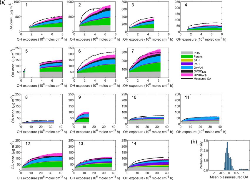
G. Stefenelli et al.: Secondary organic aerosol formation from combustion of biomass                                         11463

parameters for chemical transport models (CTMs) were not            Bertrand et al., 2017, 2018a) and are summarized here. Ex-
determined. Based on the same experiments, the lumped con-          periments from Bertrand et al. (2017, 2018a) will be referred
centrations of the 22 non-traditional volatile organic com-         to as Set 1 and experiments from Bruns et al. (2016) and Cia-
pounds and two compound classes were constrained in a box           relli et al. (2017a) as Set 2.
model (Ciarelli et al., 2017a). Improved parameters were re-           The emissions were generated by three different log wood
trieved describing the volatility distributions and the produc-     stoves for residential wood combustion: stove 1 manufac-
tion rates of oxidation products from the overall mixture of        tured before 2002 (Cheminées Gaudin Ecochauff 625), stove
precursors present in biomass smoke. While this method is           2 fabricated in 2010 (Invicta Remilly) and stove 3 (Avant,
well suited for CTMs (Pandis et al., 2013; Ciarelli et al.,         2009, Attika). For each stove three to four replicate exper-
2017b), it does not provide any information about the contri-       iments were performed with a loading of 2–3 kg of beech
butions of the different chemical classes to the aerosol. Sim-      wood having a total moisture content ranging between 2 %
ilar limitations are associated with the study of other emis-       and 19 %. The fire was ignited with three starters made of
sions, e.g. fossil fuel combustion or evaporation (Jathar et al.,   wood wax, wood shavings, paraffin and five types of natu-
2013, 2014b). The development of models capable of simu-            ral resin. The starting phase was not studied. In total, 14 ex-
lating the contribution of the different chemical species to        periments were performed, consisting of two experiments at
the aerosol at different conditions is especially important in      −10 ◦ C, seven experiments at 2 ◦ C and five experiments at
the light of the current development of highly time resolved        15 ◦ C. These experiments cover the typical range of Euro-
chemical ionization mass spectrometry, capable of quantify-         pean winter temperatures and are summarized in Table 1.
ing these products. To realize the full potential of the data          Ward and Hardy (1991) define the flaming and smoldering
acquired by this instrumentation, a modelling framework ca-         conditions according to the modified combustion efficiency,
pable of predicting the production rates and the partitioning       MCE = CO2 /(CO+CO2 ). Specifically, MCE > 0.9 is identi-
between the gas and the particle phases of the oxidation prod-      fied as the flaming condition, while MCE < 0.85 is identified
ucts from complex emissions is required.                            as the smoldering condition. MCE values for the different ex-
   Here, we extend the past analysis investigating the most         periments are reported in Table 1. According to this param-
recent smog chamber data of residential wood combustion             eter, Set 1 and Set 2 experiments were dominated by smol-
based on 14 experiments performed in 2014–2015 under var-           dering and flaming, respectively. Practically, we achieved the
ious conditions. Different experimental temperatures of the         different burning conditions by varying the amount of air in
smog chamber were investigated, namely −10, 2 and 15 ◦ C.           the stoves, therefore changing the combustion temperature.
Three different stove types were tested, including conven-          For Set 1, closing the air window decreased the flame tem-
tional and modern residential burners. Different emission           perature, resulting in a transition from a flaming to a smol-
load and different hydroxyl (OH) radical exposure were ex-          dering fire. This could be visibly identified, together with the
amined. Moreover distinct combustion regimes were sam-              development of a thick white smoke from the chimney. We
pled across the different experiments for the first time to in-     note that this conduct is very common in residential stoves,
vestigate the secondary organic aerosol chemical composi-           to keep the fire running for longer. Meanwhile, for Set 2, af-
tion and yields from flaming and smoldering emissions. Inte-        ter lighting the fire, we kept a high air input to maintain a
grated VBS-based model and novel parameterization meth-             flaming fire. At the same time, we monitored the MCE in
ods based on a genetic algorithm (GA) approach were devel-          real time and only injected the emissions into the chamber
oped to predict the contribution of the oxidation products of       when the MCE increased above 0.9.
different chemical classes present in complex emissions and            The experiments were performed in a flexible Teflon bag
to better explain the SOA formation process, providing use-         of nominally 7 but typically about 5.5 m3 equipped with
ful information to regional air quality models. Overall, this       UV lamps (40 lights, 90–100 W, Cleo Performance, Philips,
study presents a general framework which can be adapted             wavelength λ < 400 nm) enabling photo-oxidation of the
to assess SOA closure for complex emissions from different          emissions (Platt et al., 2013; Bruns et al., 2015). The cham-
sources.                                                            ber is located inside a temperature-controlled housing. Rel-
                                                                    ative humidity was maintained at 50 % and three different
                                                                    temperatures were investigated. Emissions from the stoves
2     Methods                                                       were sampled from the chimney into the chamber through
                                                                    heated (140 ◦ C) stainless-steel lines to reduce the loss of
2.1    Smog chamber set-up and procedure                            semi-volatile compounds. An ejector dilutor was installed
                                                                    (Dekati Ltd, DI-1000) to dilute emissions in the chamber by
Two smog chamber campaigns were conducted to investi-               a factor of 10 before sampling. The sample injection lasted
gate SOA production from multiple domestic wood combus-             for approximately 30 min for each experiment, and was fol-
tion appliances as a function of combustion phase, initial fuel     lowed by an injection of 1 µL d9-butanol (98 %, Cambridge
load and OH exposure. These experiments were previously             Isotope Laboratories), which was used to estimate the OH ex-
described in detail (Bruns et al., 2016; Ciarelli et al., 2017a;    posure as described in Sect. 3.1.1 (Barmet et al., 2012). The

www.atmos-chem-phys.net/19/11461/2019/                                            Atmos. Chem. Phys., 19, 11461–11484, 2019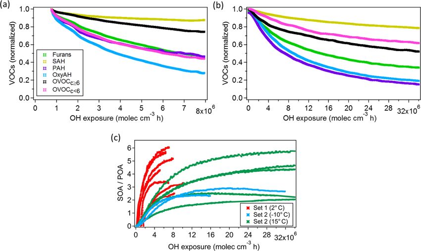
11464                                      G. Stefenelli et al.: Secondary organic aerosol formation from combustion of biomass

Table 1. Experimental parameters for the 14 smog chamber experiments used in this study, including smog chamber temperature, stove type,
modified combustion efficiency (MCE), and the initial concentrations of POA and OGs.

                                                                          Experimental     Stove                POA          OGs
          Expt.      Dataset   Reference                 Date          temperature (◦ C)   type      MCE    (µg m−3 )   (µg m−3 )
          1                    Bertrand et al. (2017)    29 Oct 2015                  2    stove 1   0.85        126        4039
          2                    Bertrand et al. (2017)    30 Oct 2015                  2    stove 1   0.84        179        7862
          3                    Bertrand et al. (2017)    4 Nov 2015                   2    stove 1   0.83         73        3694
          4          Set 1     Bertrand et al. (2017)    5 Nov 2015                   2    stove 1   0.91         10         948
          5                    Bertrand et al. (2017)    6 Nov 2015                   2    stove 2   0.80         42        1839
          6                    Bertrand et al. (2017)    7 Nov 2015                   2    stove 2   0.87         35        2007
          7                    Bertrand et al. (2017)    9 Nov 2015                   2    stove 2   0.82         44        3379
          8                    Bruns et al. (2016),      2 Apr 2014                −10     stove 3   0.97          9         301
                               Ciarelli et al. (2017a)
          9                    Bruns et al. (2016),      17 Mar 2014               −10     stove 3    NA          12        1024
                               Ciarelli et al. (2017a)
          10         Set 2     Bruns et al. (2016)       25 Mar 2014                 15    stove 3   0.97         22         526
          11                   Bruns et al. (2016)       27 Mar 2014                 15    stove 3   0.97         15         645
          12                   Bruns et al. (2016)       28 Mar 2014                 15    stove 3   0.97         17        1368
          13                   Bruns et al. (2016)       29 Mar 2014                 15    stove 3   0.97         18        1096
          14                   Bruns et al. (2016)       30 Mar 2014                 15    stove 3   0.97         18         910

        NA: not available.

chamber was then allowed to equilibrate for 30 min to en-                 2.2   Instrumentation
sure stabilization and homogeneity and to fully characterize
the primary emissions before ageing. OH radicals were pro-                We characterized the emissions with a suite of gas- and
duced by UV irradiation of nitrous acid (HONO) injected af-               particle-phase instrumentation. Organic gases (OGs) were
ter chamber equilibration, generated as described in Taira and            measured by a proton-transfer-reaction time-of-flight mass
Kanda (1990) by reaction of diluted sulfuric acid (H2 SO4 )               spectrometer (PTR-ToF-MS 8000, Ionicon Analytik). A de-
and sodium nitrate (NaNO2 ) in a gas flask followed by trans-             tailed description of the instrument can be found in Jordan
portation into the chamber with a carrier gas with a flow rate            et al. (2009). The PTR-ToF-MS was operated under stan-
of 1 L min−1 . The smog chamber was then irradiated with                  dard conditions (ion drift pressure of 2.2 mbar and drift in-
UV lights for approximately 4 h to simulate atmospheric age-              tensity of 125 Td) in H3 O+ mode, allowing the detection of
ing.                                                                      OGs with a proton affinity higher than that of water. Quan-
   Before and after each experiment, the smog chamber                     tification was performed by using known individual reac-
was cleaned with humidified pure air (100 % RH) and O3                    tion rate constants (Cappellin et al., 2012), otherwise a value
(1000 ppm) under irradiation with UV lights for at least 1 h,             of 2 × 10⁻⁹ cm3 s−1 was assumed. The effective rate con-
followed by flushing with pure dry air for at least 10 h. The             stants applied to both Set 1 and Set 2 can be found in Bruns
background particle- and gas-phase concentrations were then               et al. (2017). Data were analysed using the Tofware soft-
measured in the clean chamber.                                            ware 2.4.2 (PTR module as distributed by Ionicon Analytik
   The total amount and composition of the emissions depend               GmbH, Innsbruck, Austria) running in Igor Pro 6.3.
on the oxygen supply, temperature, fuel elemental composi-                    Non-refractory primary and aged particle composition was
tion and combustion conditions, which can be broadly classi-              monitored by a high-resolution time-of-flight aerosol mass
fied as flaming or smoldering (Koppmann et al., 2005; Seki-               spectrometer (HR-ToF-AMS, Aerodyne Research Inc.) (De-
moto et al., 2018). Flaming combustion occurs at high tem-                Carlo et al., 2006). The HR-ToF-AMS is described in detail
perature and consists of volatilization of hydrocarbons from              elsewhere (Bruns et al., 2016; Bertrand et al., 2017) and sum-
the thermal decomposition of biomass leading to rapid oxi-                marized here. The instrument was operated under standard
dation and efficient combustion, producing CO2 , water and                conditions (temperature of vaporizer 600 ◦ C, electronic ion-
black carbon (BC). Instead, smoldering combustion is flame-               ization (EI) at 70 eV, V mode) with a temporal resolution of
less and can be initiated by weak sources of heat and re-                 10 s. Data analysis was performed in Igor Pro 6.3 (Wave Met-
sults in less efficient combustion of fuel, leading to gas-phase          rics) using SQuirrel 1.57 and Pika 1.15Z assuming a collec-
products (mainly CO, CH4 and volatile organic compounds).                 tion efficiency of 1. The O : C ratio was determined according
                                                                          to Aiken et al. (2008).

Atmos. Chem. Phys., 19, 11461–11484, 2019                                                  www.atmos-chem-phys.net/19/11461/2019/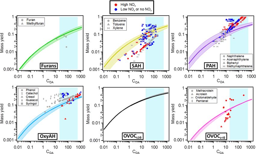
G. Stefenelli et al.: Secondary organic aerosol formation from combustion of biomass 11465
The concentration of equivalent black carbon (eBC) glected their production from other OGs (i.e. P = 0). This as-
was determined from the absorption coefficient measured sumption signifies that the yields estimated under our condi-
with a seven-wavelength Aethalometer (Magee Scientific tions are upper limits. In reality, the detection of aromatic hy-
Aethalometer model AE33) with a time resolution of 1 min drocarbons (e.g. single-ring aromatic hydrocarbons, SAHs,
at a wavelength of 880 nm (Drinovec et al., 2015). and polycyclic aromatic hydrocarbons, PAHs) by the PTR-
The particle number concentration and size distribution ToF-MS may be affected by the interference due to fragmen-
(16 to 914 nm) were provided by a scanning mobility particle tation during ionization of their oxidation products (Guen-
sizer (SMPS, consisting of a custom-built differential mo- eron et al., 2015). On the other hand, directly emitted oxy-
bility analyser (DMA) and a condensation particle counter genated aromatics could themselves be the oxidation prod-
(CPC 3022, TSI)) with a time resolution of 5 min. Support- ucts of aromatic hydrocarbons and their production may con-
ing gas measurements included a CO2 analyser (LI-COR), a tinue during the experiment. However, the assumption of
CH4 monitor, a total hydrocarbon (THC) monitor (flame ion- P = 0 does not introduce a significant error for most OGs
ization detector, THC monitor Horiba APHA-370), and NO with significant primary emissions because the observed OG
and NO2 (NOx analyser, Thermo Environmental) monitors. decay was consistent with their OH reaction rate constant for
Set 2 as demonstrated by Bruns et al. (2017) for the +15 ◦ C
conditions. In the following, we describe the processes gov-
3 Data analysis erning the changes in the OG concentrations in the chamber
and the approaches adopted for the determination of the dif-
The data analysis entails three steps detailed in this sec-
ferent parameters in Eq. (1).
tion. The first subsection describes the determination of the
amount of oxidized OGs in the chamber. The second subsec- 3.1.1 Reaction with OH radical
tion details the determination of the amount of SOA formed
in the chamber. The last subsection describes the box model The OH exposure, which is the integrated OH concentration
used for the parameterization of SOA formation from the over time, was estimated based on the differential reactivity
OGs. of two OGs. Specifically, we used d9-butanol (fragment at
mass-to-charge ratio m/z 66.126, [C4 D9 ]+ ) and naphthalene
3.1 Organic gas loss in the chamber
(fragment at m/z 129.070, [C10 H8 ]H+ ). These compounds
are selected because they can be unambiguously detected (no
In the chamber, OGs were oxidized to several oxidation prod-
isomers or interferences, high signal-to-noise ratio), are not
ucts, referred to as oxidized OGs (CG, condensable gases)
produced during the experiment and have OH reaction rate
in the following analysis. According to their volatility, these
constants that are precisely measured and significantly dif-
products may remain in the gas phase or partition to the par-
ferent from each other. The OH exposure can be expressed
ticle phase, thereby contributing to SOA formation.
as follows:
We described the change in any OG concentration over
time as a combination of its loss and production as follows:
d9−butanol
d9−butanol
ln naphthalene − ln naphthalene
0 t
OH exposure = , (2)
d[OG] kOH,but − kOH,naph
= P−
dt
X
kdil × [OG] + kOH × [OH] × [OG] + kother × [OG] . where (d9-butanol / naphthalene)0 is the ratio between
(1) these compounds at t = 0 (before lights were turned
on), (d9-butanol / naphthalene)t is the ratio measured at
Here, P corresponds to the production of an OG in the time t, and kOH,but and kOH,naph are the OH reaction
chamber, e.g. from the oxidation of other primary OGs. kdil rate constants of d9-butanol and naphthalene, respectively
is the dilution rate constant in reciprocal seconds. kOH [OH] (kOH,but = 3.14 × 10⁻¹² cm3 molec.−1 s−1 and kOH,naph =
[OG] in molecules per cubic centimetre per second repre- 2.30 × 10⁻¹¹ cm3 molec.−1 s−1 ) (Atkinson and Arey, 2003).
sents the consumption rate due to oxidation by OH, where For Set 1, the OH exposure at the end of each experi-
kOH is the reaction rate constant and [OH] is the OH con- ment ranged between 5 and 8 × 10⁶ molec. cm−3 h, corre-
centration. kother [OG] in molecules per cubic centimetre per sponding to approximately 5–8 h in the atmosphere (given
second is the loss rate of OG by other processes, where kother global average and typical wintertime OH concentrations of
is the reaction rate constant in reciprocal seconds. The loss 1 × 10⁶ molec. cm−3 ). For Set 2, higher OH exposures were
of some OGs could not be explained by their reaction with reached (3 to 7 × 10⁷ molec. cm−3 h at the end of each ex-
OH and dilution alone for Set 1, so we added this additional periment, corresponding to 2–3 d in the atmosphere). This
term, which is discussed after the first two processes are con- is likely because both sets of experiments utilized a similar
strained. We considered primary OGs that exhibited a clear HONO molar flow (and thus similar OH production rate),
decay with time to be strictly of primary origin, and hence ne- but higher OG concentrations were reached in Set 1, which
www.atmos-chem-phys.net/19/11461/2019/ Atmos. Chem. Phys., 19, 11461–11484, 2019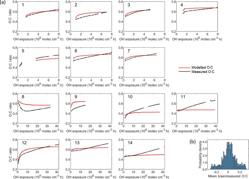
11466                                 G. Stefenelli et al.: Secondary organic aerosol formation from combustion of biomass

could possibly have resulted in a higher OH sink. We calcu-          3.1.4   Precursor classification
lated the OH concentration, [OH] in Eq. (1), numerically as
d(OH exposure)/dt.                                                   A common set of 263 ions was extracted from the PTR-ToF-
                                                                     MS. Among these ions, 86 showed a clear decay with time
3.1.2    Smog chamber dilution                                       and were thus identified and selected as potential SOA pre-
                                                                     cursors. Previous work based on Set 2 experiments showed
For Set 2, dilution was dominated by the constant injection          that the PTR-ToF-MS measures the most important SOA pre-
of HONO to the chamber and accounted for as described in             cursors, which explained the measured SOA mass within
Bruns et al. (2016). For Set 1 the dilution rate of primary          40 % uncertainty and without systematic bias (Bruns et al.,
OGs in the chamber was calculated as follows. The inte-              2016). Therefore, these compounds are expected to capture
grated dilution over time, Kdil , was determined as the ratio        the dominant fraction of SOA mass, although we cannot
between the d9-butanol concentration corrected for the reac-         rule out losses in the PTR-ToF-MS inlet or small contri-
tion of d9-butanol with OH and the d9-butanol concentration          butions from other precursors such as alkanes. The com-
at t = 0([d9−butanol]0 ):                                            pound identification was supported by previous publications
                                                                     (McDonald et al., 2000; Fine et al., 2001; Nolte et al.,
         [d9−butanol] × ekOH,but ×OH exposure                        2001; Schauer et al., 2001; Stockwell et al., 2015), including
Kdil =                                        .               (3)
                 [d9−butanol]0                                       gas chromatography–mass spectrometry (GC–MS) analysis
                                                                     when available.
   Figure S1 shows calculated values for Kdil as a function
                                                                        The size of our dataset does not allow us to retrieve the
of time. Increasingly high dilution at the end of these experi-
                                                                     volatility distribution for single precursors, which would
ments (Fig. S1), between 20 % and 35 % (i.e. a dilution ratio
                                                                     entail the determination of more than 86 free parameters.
of 0.8 to 0.65), is a result of constant injection of HONO
                                                                     This is especially the case as the time series of precursors,
and excessive sampling at high rates, resulting in inputs from
                                                                     decaying with oxidation, are typically strongly correlated,
laboratory air (likely through leaks in the Teflon bag or the
                                                                     which prevents resolving systematic differences between the
connections of chamber inlets and outlets). The inputs from
                                                                     yields of the different single precursors. Therefore, lumping
the HONO pure carrier gas and of laboratory air are roughly
                                                                     is needed to decrease the model degree of freedom. Accord-
comparable (about 12 % vs. 8 %–23 % at the end of the ex-
                                                                     ingly, precursors are grouped in six chemical classes: furans,
periment). Other than dilution, the effect of both inputs on the
                                                                     single-ring aromatic hydrocarbons (SAHs), polycyclic aro-
gas-phase chemical composition is negligible. Dilution rates
                                                                     matic hydrocarbons (PAHs), oxygenated aromatics (OxyAH)
are non-linear, increasing as the experiment progresses due
                                                                     and organic compounds containing six and more or fewer
to continuous dilution within a decreasing chamber volume.
                                                                     than six carbon atoms (OVOCc ≥ 6 and OVOCc < 6 , respec-
The dilution rate constant, kdil , in Eq. (1), is the differential
                                                                     tively) (Table S1). The selected precursors in each class are
of Kdil over time.
                                                                     the same for each experiment and each dataset. This lumping
3.1.3    Losses by other processes                                   approach is based on the two main objectives of the study:
                                                                      1. Compare the SOA yields of specific precursors deter-
To corroborate the estimated OH exposures and dilution                   mined in complex emission experiments with those de-
rates, we examined the loss of prominent OGs with known                  termined in single-compound systems.
reaction rate constants against OH. For Set 2 and as demon-
strated by Bruns et al. (2017), the OG decay is consistent            2. Identify the main SOA precursors in flaming and smol-
with their estimated loss based on their dilution and reac-              dering wood emissions, at different temperatures.
tion with OH. By contrast, for Set 1, the decay of some OGs             To be able to compare to literature yields, we lumped
could not be solely explained by their reaction with OH and          species that have similar yields in the same chemical class:
dilution, suggesting additional reactions with oxidants other        e.g. at an organic aerosol concentration of 10 µg m−3 the
than OH as discussed
               R         below.
                             The OG total consumption by            yield of PAHs is ∼ 20 % (objective 1). In addition, we clas-
this process     kother [OG] was estimated as the difference         sified the precursors based on the pathway by which they
between the total measured decay of the OG of interest and           are emitted, which will allow us to determine which com-
the fraction consumed by both dilution and oxidation by OH           pounds dominate SOA formation in flaming and smolder-
radicals. The reaction rate constants for several precursors         ing emissions (objective 2). We differentiated between oxy-
towards OH (kOH ) are not available in the literature. In ad-        genated aromatics, mainly emitted through lignin pyrolysis,
dition, many fragments may have several isomers, each of             furans emitted through cellulose pyrolysis, and single-ring
which is associated with different rate constants. Effective         aromatics and PAHs generated from incomplete combustion,
rate constants for all precursors considered were estimated          especially from flaming wood. The remaining SOA precur-
from their decay in Set 2, where the combination of OH re-           sors are all oxygenated OGs; therefore we separated them
action and dilution fully explained the decay of OGs with            according to their carbon number knowing that larger pre-
known OH reaction rate constants.                                    cursors will have higher yields than smaller precursors. Our

Atmos. Chem. Phys., 19, 11461–11484, 2019                                           www.atmos-chem-phys.net/19/11461/2019/
G. Stefenelli et al.: Secondary organic aerosol formation from combustion of biomass                                          11467

ability to precisely extract yields specific to a precursor class    estimated that at 293 K the fraction of these compounds ab-
heavily relies on differences in the oxidation rates or emis-        sorbed on the walls is < 5 %. Meanwhile, the walls could
sion patterns of the precursors. Therefore, the classification       indeed act as a sink for the semi-volatile oxidation products.
approach adopted here, where classes are expected to have            This effect was not taken into account in the current study,
different contributions during different experiments (Bhattu         but we expect that it was minimized under our conditions, by
et al., 2019), facilitates the extraction of yields of the differ-   the high OA concentration in the chamber and high produc-
ent classes.                                                         tion rates (Zhang et al., 2014; Nah et al., 2017).

3.2   Calculation of the OA mass in the chamber                      3.3     Modelling SOA formation
The total organic aerosol measured by the HR-ToF-AMS was             The general aim of the model is the determination of the
corrected for particle losses in the chamber due to gravi-           parameters describing the volatility distributions of the ox-
tational and diffusional deposition. To assess the total wall        idation products from different precursor classes and their
losses due to both processes, we assumed that the condens-           temperature dependence. A simplified schematic of the mod-
able vapours partition only to the suspended aerosols but not        elling framework is described in Fig. 1. It consists of (1) a
to the wall.                                                         box model that describes the partitioning of the condens-
   Assuming that black carbon is inert in the chamber, it was        able gases generated through oxidation, (2) the model input
possible to use its decay to estimate the particle loss to the       parameters obtained from the smog chamber, (3) the model
walls. The aerosol attenuation measured at 880 nm (at the end        output parameters and (4) the model optimization based on
of each experiment, ∼ 4 h) with an Aethalometer was used to          a genetic algorithm (GA). Each of these parts is described in
estimate the particle loss rate to the wall. This attenuation is     the following sections.
proportional to the eBC mass concentration and within un-
certainties independent of the ageing extent, as demonstrated        3.3.1    Box model
in Kumar et al. (2018). Using eBC as a tracer, we inherently
assumed that eBC and OA were internally mixed and homo-              We assume the partitioning of CG between the gas and the
geneously distributed over the aerosol size range. The decay         particle phases to obey Raoult’s law (Strader et al., 1999),
of eBC due to both dilution and deposition onto the chamber          where the aerosol can be described as a pseudo-ideal organic
walls was parametrized as follows:                                   solution, of SOA and POA species. The volatility basis set
d[eBC]                                                               (VBS, implemented by Koo et al., 2014, in the Comprehen-
       = −kdil [eBC] − kwall [eBC],                           (4)    sive Air quality Model with eXtensions, CAMx) was used
  dt
                                                                     to classify the oxidation products of the different precursors
where kwall is the first-order wall loss rate constant used to       into surrogates with different volatility, distributed into dis-
correct the measured OA concentration for wall losses, rang-         crete logarithmically spaced bins (Donahue et al., 2006).
ing between 4 and 8 × 10⁻⁵ s−1 , and kdil is the dilution rate          We considered the most basic mechanism by which SOA
constant determined above.                                           may form. That is, the oxidation products from the different
  The wall-loss-corrected organic aerosol, OAWLC , was cal-          precursor classes described above instantaneously partition
culated using Eq. (5):                                               into the condensed phase depending on their volatility. No
                        Zt                                           additional reactions in the gas or particle phase were consid-
OAWLC (t) = OA(t) +          kwall × OA(t) × dt,              (5)    ered (e.g. reaction with oxidants, photolysis or oligomeriza-
                                                                     tion). In addition, we neglected the contribution of primary
                         0
                                                                     oxidation products of the gas-phase semi-volatile species
where OA(t) is the measured organic aerosol concentration            (co-emitted with POA) compared to the OGs detected by the
in microgram per cubic metre. The total OA present in the            PTR-ToF-MS, based on the findings of Bruns et al. (2016)
chamber was estimated as the suspended OA concentration              and Ciarelli et al. (2017a). Finally, we considered the species
measured by the HR-ToF-AMS plus the estimated OA lost                in the gas and the particle phases to be permanently at equi-
to the wall. This concentration was directly compared to             librium, as condensation is expected to be faster than oxida-
the condensable gas (CG) concentration estimated accord-             tion (timescales for oxidized vapour condensation < 1 min
ing to Eq. (A8) presented in Appendix A. As mentioned, our           assuming no particle-phase diffusion limitations; Bertrand
approach did not take into account the losses of precursor           et al., 2018b). While including additional processes in the
vapours or their oxidation products in the gas phase onto the        model is feasible, this would result in a significantly higher-
walls. We note that these processes were unlikely to have a          dimensional parameter space, which cannot be unambigu-
substantial effect on the precursors considered, which were          ously inferred from the present data. We consider that with-
largely highly volatile species, even at lower temperature.          out supportive data, e.g. chemically resolved characteriza-
Based on the calculation of the equilibrium constant of semi-        tion of the particle-phase species, such reactions could not
volatile species on the walls by Bertrand et al. (2018b), we         be well constrained or even deduced from structure activity

www.atmos-chem-phys.net/19/11461/2019/                                             Atmos. Chem. Phys., 19, 11461–11484, 2019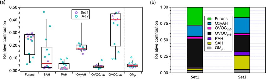
11468                                  G. Stefenelli et al.: Secondary organic aerosol formation from combustion of biomass

Figure 1. Schematic of the modelling framework. The box model simulates the formation of SOA from each precursor class j in volatility
bins i. The best solution of the initialized input parameter volatility distribution (described as the mean value of logC* for each precursor
class µj and standard deviation σ ) and enthalpy of vaporization (1Hvap ) parameters are optimized by a genetic algorithm, using minimum
mean bias and root-mean-square error (RMSE) between modelled and measured OA concentration as the fitness function. Green boxes
represent measured data from the chamber experiments.

relationships, given the many unknowns in complex emis-                  3.3.2   Model inputs
sions. Therefore, such a simplified scheme of SOA formation
from complex emissions may be compared in the future with                The model uses as main inputs the molar concentrations
chemically resolved data to help the identification of addi-             of the condensable gases from different precursors (in to-
tional mechanisms that were not considered here.                         tal n = six precursor classes) in both phases, xj |g + p . The
   The derivation of the thermodynamic equations govern-                 concentration of condensable gases in both the gas and
ing SOA formation from precursors, implemented in the box                particle phases is derived from the consumption rates of
model, is detailed in Appendix A and only a brief description            VOCj determined by the PTR-ToF-MS, by numerically
of the model principles is given here. In the following, let i           integrating Eq. (A8). xj |g + p is related to the concentra-
and j be the indices for the different volatility bins and pre-          tions of the different surrogates from a precursor class j
cursor classes, respectively. The model determines the molar             in different volatility bins, xi,j |g + p (Eq. A6), through their
distribution of the oxidation products from different precur-            yields, ϒi,j , according to Eq. (A9). The number of volatil-
sor classes in the different volatility bins, ϒi,j , together with       ity bins, m, is set to six, approximately corresponding to the
                                                                         following mass saturation concentrations: Ci,j    ∗ µg m−3 =
the compounds’ enthalpy of evaporation, 1Hvap,i,j . The lat-
                                                                           10 ; 100 ; 101 ; 102 ; 103 ; 104 .
                                                                          −1
ter describes the temperature dependence of the oxidation
products’ effective molar saturation concentration, xi,j   ∗ . For                                                                 OM
                                                                            In addition to xj |g + p , the model needs as input xi p |p+g ,
this, the model iteratively solves Eqs. (A6) and (A7) at ev-             the molar concentration of primary organic matter from a
ery experimental time step (time resolution of 10 s) for all             volatility bin i in both gas and particle phases (Eq. A7).
experiments, to retrieve the surrogate molar concentrations                OM
                                                                         xi p |g + p is inferred from the measured POA concentrations
in the particle phase, xi,j |p , and the total surrogates’ molar
                                                                         injected in the chamber at the beginning of the experiment
concentration in the condensed organic phase, xOA (see Ap-
                                                                         and using the volatility distribution function of wood com-
pendix A).
                                                                         bustion emissions in May et al. (2013). It is assumed con-
                                                                         stant with ageing. The computation of the fraction of POAi
                                                                         in the condensed phase is similar to that for SOA species in
                                                                         Eq. (A6).

Atmos. Chem. Phys., 19, 11461–11484, 2019                                                 www.atmos-chem-phys.net/19/11461/2019/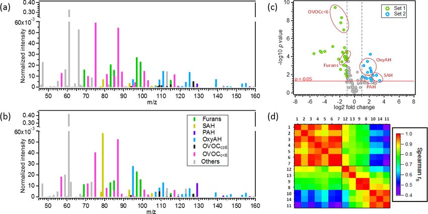
G. Stefenelli et al.: Secondary organic aerosol formation from combustion of biomass                                            11469

   The secondary surrogates’ elemental composition (C#i,j ,
O#i,j and H #i,j ) is also used as model input to compute
                                                                               n P                             OMp OMp
the surrogates’ molecular weight, MWi,j , required for COA                     P   m
                                                                                        O#i,j xi,j       + O#i    xi
                                                                                    i
calculations (see Sect. 3.3.3). A single C#i,j value is cal-                    j                    p
                                                                                                                       p
culated per chemical class, based on the average C#VOC     j
                                                                     O:C=                                                   .     (7)
                                                                                n P                            OM OM
of the respective precursor class, and considering C#i,j =                            m
                                                                                                             C#i p xi p
                                                                                P
                                                                                      i C#i,j xi,j       +
C#VOC
    j    − 1C, where 1C is the average loss in carbon due                       j                    p
                                                                                                                        p
to fragmentation during the oxidation of precursors from all
classes. 1C is determined by systematically changing its             3.3.4    Model optimization
value in multiple model runs and selecting the value that
best explains the observed O : C ratios (see Fig. 8b). Like-         The model is optimized to determine the volatility distri-
wise, a single H #i,j value is assumed per chemical class,           butions of the oxidation products from different precursor
considering that H #j /C#j equals H #VOC     /C#VOC   . Finally,     classes described by µj , σ and their temperature depen-
                                         j        j
O#i,j is constrained by the C#j and the surrogate volatil-           dence described by 1Hvap to best fit the observed OA con-
        ∗ ) based on the simplification of the SIMPOL model
ity (Ci,j                                                            centrations. For the model optimization, we used a genetic
(Pankow and Asher, 2008), provided by Eq. (3) in Donahue             algorithm (GA), a metaheuristic procedure inspired by the
et al. (2011). Based on this relationship, O#i,j increases with      theory of natural selection in biology, including selection,
decreasing C#j and Ci,j  ∗ . The O : C ratio of primary emis-        crossover and mutation processes, to efficiently generate
sions is constrained in the model to the measured O : C in the       high-quality solutions to optimize problems (Goldberg et al.,
beginning of each experiment, by setting C#OMp and calcu-            2007; Mitchell, 1996). The GA is initiated with a population
            OM                                                       of randomly selected individual solutions. The performance
lating O#i p using the same methodology as for O#i,j . The
                           OMp                                       of each of these solutions is evaluated by a fitness function,
resulting C#OMp and O#i              and the corresponding primary   and the fitness values are used to select more optimized solu-
                                             OM
organic matter molecular weight, MWi p , as well as C#j ,            tions, referred to as parents. The new generation of solutions
O#i,j , H #j and MWi,j , is reported in Table S4.                    (denoted children) is produced by either randomly changing
                                                                     a single parent (as mutation) or combing the vector entries of
3.3.3   Model outputs                                                a pair of parents (as crossover). The evolution process will be
                                                                     repeated until the termination criterion is reached, here maxi-
The model provides the ϒi,j and 1Hvap,i,j parameters. To             mum iteration time. In this study, a population of 50 different
reduce the model’s degree of freedom we consider a sin-              sets of model parameters (µj , σ and 1Hvap ) was considered
gle 1Hvap for all surrogates from different chemical classes         for each GA generation. The sum of mean bias and RMSE
in different volatility bins. ϒi,j is considered to follow a         between measured and modelled COA of the 14 experiments
kernel normal    distribution as a function of log C ∗ , ϒi,j ∼      was used as a fitness function to evaluate the solutions. We
N µj , σ , where µj is the median value of log C ∗ and σ

                                                                     assume the termination criterion is reached if no improve-
is the standard deviation. This step (1) ensures positive ϒi,j       ment in the fitness occurs after 50 generations, with a max-
parameters, (2) significantly reduces the model’s degree of          imum of 500 total iterations allowed. The GA calculations
freedom and (3) allows constraint of the total
                                             P concentration         were performed using the package “GA” for R (Scrucca et
of surrogates from a certain chemical class: m   i ϒi,j = 1.         al., 2017). A bootstrap method was then adopted to quantify
   The set of ϒi,j and 1Hvap,i,j parameters is determined            the uncertainty in the constrained parameters.
by minimizing the sum of mean bias (MB) and the root-
mean-square error (RMSE) between modelled mass concen-
trations of the particulate organic phase, COA , calculated us-      4     Results and discussion
ing Eq. (6), and concentrations measured by the AMS.
                                                                     4.1     Comparison of primary emissions across
        n X
        X  m                               OMp OMp
                                                                             experiments
COA =           i
                    MWi,j xi,j       + MWi    xi               (6)
                                                   p
         j                       p                                   A larger amount of primary OG was emitted into the cham-
                                                                     ber in Set 1, with concentrations ranging from 950 to
   The model fitted to the measured COA was also validated           7860 µg m−3 , while in Set 2 the primary OG concentrations
by external AMS measurements of the O : C ratio determined           ranged from 300 to 1360 µg m−3 . In the same way, the mea-
through high-resolution analysis. The modelled O : C ratio           sured OA at the beginning of each test (POA) ranged from
was calculated at every experimental time step as follows:           10 to 180 µg m−3 and from 9 to 22 µg m−3 for Set 1 and
                                                                     Set 2, respectively (Table 1). The OG composition for Set 1
                                                                     and Set 2 is summarized in Fig. 2 showing the mean PTR-
                                                                     ToF-MS mass spectra (Fig. 2a, b), the relative contributions
                                                                     of the different compounds for different datasets (Fig. 2c)

www.atmos-chem-phys.net/19/11461/2019/                                              Atmos. Chem. Phys., 19, 11461–11484, 2019
11470 G. Stefenelli et al.: Secondary organic aerosol formation from combustion of biomass Figure 2. Comparison of the OG emissions between the two sets of experiments. Panels (a) and (b) display average primary OG mass spectra from Set 1 (representing the smoldering phase) and Set 2 (representing mainly the flaming phase), respectively. Spectra are normalized to the initial total OG concentration in micrograms per cubic metre. Compounds are colour coded by chemical classes. (c) The p value vs. fold change comparing the fingerprints of primary OGs between the two sets of experiments. The fold change was calculated as the ratio of the intensities of each ion normalized to the total signal, between Set 2 and Set 1 averaged across experiments. Data points above p = 0.05 have significantly different contributions to the total OGs between the two sets of experiments. Blue coloured data points on the right-hand side designate compounds enriched in the emissions from Set 2 while green coloured data points on the left-hand side designate compounds enriched in the emissions from Set 1. (d) Spearman correlation matrix for the primary OG mass spectra between all experiments highlighting the variability in the composition of the primary emissions. Each experiment is identified by an index (see Table 1) and the experiments from Set 2 were reordered according to similarity with Set 1. and the variability in composition among all experiments discrepancy was the difficulty in injecting flaming emissions (Fig. 2d). Set 1 shows higher relative contributions of furans without any significant smoldering contribution for Set 2. and OVOCc < 6 (Fig. 2a), while the contributions of PAH, This hypothesis is supported by the strong similarity between SAH and OxyAH are higher in Set 2 (Fig. 2b). The OxyAH precursor compounds measured in some experiments sup- compounds, mainly methyl- and methoxyphenols, are pro- posed to represent flaming-phase emissions only but appar- duced by lignin pyrolysis (Fine et al., 2001) while furans ently included some smoldering as well (9, 12, 13) and exper- are formed from cellulose pyrolysis (Mettler et al., 2012). iments from Set 1 (1–7). Figure S2 reports the relative contri- The chemical class referred to as “Others” comprises com- butions of primary OGs (before photo-oxidation) for all com- pounds that do not show a clear decay upon oxidation and pound classes for the 14 experiments. Note that these trends are therefore not considered SOA precursors in the follow- are not correlated with the modified combustion efficiency ing analysis. The category others is dominated by acetic acid, (MCE), reported in Table 1, defined as CO2 /(CO + CO2 ), previously reported as a major species in residential wood which was constant at 0.97 g g−1 , for Set 2, but ranged from burning emissions (Bhattu et al., 2019). The majority of the 0.8 g g−1 to 0.91 g g−1 for Set 1. compounds differ among datasets and the most significant Figure 3 shows the contribution of each class of precursor difference estimated through the p value (probability associ- compounds and of the primary semi-volatile organic mat- ated with a Student’s t test) occurs for the OVOCc < 6 , which ter (OMP ) to the total primary emissions. OMP is the total is about a factor of 6 higher than the significance threshold organic matter in the semi-volatile and low-volatility range (p = 0.05) for Set 1. In order to investigate the similarity in the particle and the gas phases (saturation concentration between all experiments a Spearman correlation matrix was < 1000 µg m−3 at 298 K) (see Sect. 3.3.2). Overall, the high- calculated. Experiments from Set 1 appear to be consistently est average relative contributions are related to OVOCc < 6 similar to each other while the experiments from Set 2 are followed by furans and OxyAH, but we also note an aver- significantly different among each other in terms of compo- age large contribution by SAH for Set 2. The two sets of ex- sition of the primary emissions. A possible reason for such a periments investigated clearly show different primary com- Atmos. Chem. Phys., 19, 11461–11484, 2019 www.atmos-chem-phys.net/19/11461/2019/
G. Stefenelli et al.: Secondary organic aerosol formation from combustion of biomass                                                11471

Figure 3. (a) Box plot for the relative contributions to the total primary emissions of the different precursor classes and of OMp averaged
between experiments. OMp is the total semi-volatile and low-volatility organic matter calculated by means of the VBS model assuming the
volatility distribution from May et al. (2013) and using as input the measured organic aerosol (OA) mass. The top and bottom whiskers
represent the 90th and 10th percentiles, respectively, while the top, middle and bottom lines of the boxes show the 75th, 50th and 25th
percentiles, respectively. The circles represent each single experiment from the two datasets investigated. (b) Average contributions of
different precursor families and OMp for Set 1 and Set 2.

position of emissions in terms of dominant contributions; in            Table 2. Reported average reaction rate constants
Set 1 OVOCc < 6 and OxyAH dominate by far the total pri-                (10−11 cm3 molec.−1 s−1 ) towards OH per family at the be-
mary emissions while in Set 2 the main species influencing              ginning of each experiment, including average reactivity (AVG)
the total primary emissions are OxyAH, OVOCc < 6 and SAH                and standard deviation (SD).
with roughly similar contributions (see Fig. 3b). Moreover,
                                                                          Expt.   Furans     SAH    PAH    OxyAH    OVOCc = 6   OVOCc < 6
the calculated averaged OMp / OGs ratios are around 0.05
and 0.03 for Set 2 and Set 1, respectively.                               1         2.96     1.90   2.90     1.94        0.66        1.16
                                                                          2         2.97     1.86   2.99     2.05        0.70        1.25
    OGs undergo oxidation during atmospheric ageing to form
                                                                          3         3.04     1.88   2.95     2.07        0.66        1.19
a complex mixture of products, some of which remain in the                4         2.79     2.02   2.84     2.38        0.62        1.16
gas phase while others have sufficiently low volatility to par-           5         3.04     2.10   2.73     2.57        0.60        1.12
tition to the particle phase. The consumption of the differ-              6         3.04     1.88   2.83     2.09        0.59        1.11
                                                                          7         2.92     1.93   2.80     2.05        0.67        1.21
ent OG classes over time is shown in Fig. 4a, b for Set 1                 8         3.09     2.28   3.36     3.74        0.88        1.40
and Set 2, respectively. The general trends manifest that PAH             9         3.65     2.37   3.76     5.58        0.69        1.48
and OxyAH are the most reactive classes, exhibiting an av-                10        3.15     2.34   3.27     4.41        0.59        1.44
erage consumption of up to 80 % at the end of the experi-                 11        3.11     2.34   3.07     4.04        0.60        1.57
                                                                          12        3.04     2.23   2.50     2.32        0.75        1.39
ments (after ∼ 4 h of ageing) while for both datasets SAH ap-             13        3.02     2.33   3.48     2.98        0.72        1.41
pears to be the least reactive class (with an average consump-            14        2.96     2.36   3.58     4.40        0.77        1.50
tion between 10 % and 20 % at the end of the experiments).
                                                                          AVG       3.06     2.13   3.08     3.04        0.68        1.31
Relevant compounds in the latter class are benzene (C6 H6 ),              SD        0.19     0.21   0.36     1.17        0.08        0.16
toluene (C7 H8 ) and xylene (C8 H10 ); their slow reactivity is
consistent with literature reaction rate constants toward OH,
from the NIST database (NIST chemistry WebBook, Lin-
strom and Mallard, 2018), of 1.22 × 10⁻¹² , 6.13 × 10⁻¹² and               In the same way, we also observe a higher SOA production
7.51 × 10⁻¹² (cm3 molec.−1 s−1 ), respectively.                         for Set 1 compared to Set 2 at comparable OH exposure. The
    The two datasets differ for the OH dose; we observe in              SOA-to-POA ratio ranges between 2 and 6, similar to ratios
Set 2 (Expt. 8–14) an overall higher consumption of all pre-            observed in previous studies (Heringa et al., 2011; Bruns et
cursor classes due to the higher OH dose (representing a                al., 2015; Grieshop et al., 2009; Tiitta et al., 2016).
longer ageing time in an ambient atmosphere). PAH shows                    Overall the same chemical classes appear to behave dif-
the highest reactivity followed by OxyAH while for Set 1                ferently across the different sets of experiments. Such an in-
(Expt. 1–7) the fastest class of compounds to react is the              consistency in behaviour is due to either differences in the
OxyAH followed by PAH and OVOCc < 6 . Moreover, despite                 chemical composition within the same class or due to addi-
the lower OH exposure reached for Set 1, the consumption                tional reactivity occurring in Set 1.
of OxyAH and furans is substantially higher at comparable                  To investigate the chemical differences within the same
exposure levels.                                                        class of compounds across different experiments, Table 2 re-

www.atmos-chem-phys.net/19/11461/2019/                                                     Atmos. Chem. Phys., 19, 11461–11484, 2019
11472 G. Stefenelli et al.: Secondary organic aerosol formation from combustion of biomass
Figure 4. Average consumption of SOA precursor classes against average OH exposure for Set 1 (a) and Set 2 (b). The observed decay of
SOA precursor families (OGs) as described in Eq. (1) is due to both oxidation processes and dilution in the chamber. (c) SOA-to-POA ratio
for each experiment against average OH exposure coloured according to experimental temperatures (2, −10, 15 ◦ C).
Here, c represents the single compound, j the family and k
the experiment. kOH is the reaction rate constant toward OH
and OG refers to the primary OGs.
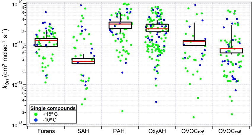
OH reaction rate constants (kOHc,j ) for each compound
were calculated from Set 2 only (Fig. 5), whereas the decay
of the precursors contributing most to SOA formation dur-
ing ageing was compared with the expected decay based on
literature. The good agreement indicates that for these exper-
iments the consumption of the precursors was dominated by
OH (Bruns et al. 2017). The average OH reaction rate con-
stants (kOHc,j ) are reported in Table S3. They are determined
for each precursor class and calculated with a first-order ex-
Figure 5. Box plot of mass-weighted average OH reaction rate con- ponential fitting on the precursors’ decay curves previously
stants (kOH ) determined for each precursor class from Bruns et corrected for dilution.
al. (2016) for Set 2 only (see Table S3). The individual kOH val-
The average reaction rate constants per family (k OHj,k ) are
ues for all compounds are also shown for all experiments, colour
similar among the same families for different experiments,
coded according to the experimental temperatures. The top and bot-
tom whiskers represent the 90th and 10th percentiles, while the top, suggesting that the variable behaviour of the chemical classes
middle and bottom lines of the boxes show the 75th, 50th and 25th across different experiments was due to differences in the re-
percentiles, respectively. active environment rather than a different chemical composi-
tion within a given class.
As introduced in Sect. 3.1.3, the total measured decay of
ports the average reaction rate constants against OH of the OGs in Set 1 could not be fully explained by dilution and re-
different chemical classes calculated at the beginning of each activity against OH, suggesting the presence of an additional
experiment following Eq. (8). loss process. To assess the remaining oxidation processes,
kOH values were used to estimate the missing loss process for
X OGc,j,k Set 1 according to Eq. (1). In this way the consumed fraction
k OHj,k = kOHc,j × (8)
i
OGj,k due to OH chemistry, dilution in the chamber and the addi-
tional reactivity was calculated for each OG compound fam-
ily and is shown in Fig. 6. The additional reactivity appears to
Atmos. Chem. Phys., 19, 11461–11484, 2019 www.atmos-chem-phys.net/19/11461/2019/You can also read