Self-fulfilling Liquidity Dry-ups - FREDERIC MALHERBE
←
→
Page content transcription
If your browser does not render page correctly, please read the page content below
Self-fulfilling Liquidity Dry-ups
                                              FREDERIC MALHERBE∗

                                            Journal of Finance forthcoming

                                                          Abstract
       This paper presents a model in which cash holding imposes a negative externality because it worsens
       future adverse selection in markets for long-term assets, which impairs their role for liquidity provision.
       Adverse selection worsens when potential sellers of long-term assets hold more cash because then fewer
       sales reflect cash needs, and proportionally more sales reflect private information. Moreover, future mar-
       ket illiquidity makes current cash holding more appealing. This feedback effect may result in hoarding
       behavior and a market breakdown, which I interpret as a self-fulfilling liquidity dry-up. This mechanism
       suggests that imposing liquidity requirements on financial institutions may backfire.

Many policy makers and academics have pointed out unusual cash hoarding behavior by major financial
institutions since the 2007-2009 financial crisis in general and a further surge in the euro area since the end
of 2011.1 Many have also expressed concerns that such behavior worsens the economic outcome2 , a topic to
which several recent academic studies have been dedicated (Diamond and Rajan (2011); Acharya and Skeie
(2011); Acharya, Shin, and Yorulmazer (2011); Gale and Yorulmazer (2012); Caballero and Krishnamurthy
(2008)). The role of adverse selection during the crisis has also been pointed out (see, for instance, Tirole
(2011b); Bolton, Santos, and Scheinkman (2011); Morris and Shin (2012)). However, that hoarding behavior
and adverse selection may reinforce each other has received little attention so far.
   ∗ London    Business School, Regent’s Park, NW1 4SA London, United Kingdom, fmalherbe@london.edu. I am deeply indebted
to an anonymous referee, an associate editor, and Campbell Harvey (the editor) for detailed feedback that greatly improved the
paper. This work is based on the first chapter of my PhD dissertation at ECARES, Université libre de Bruxelles. I am partic-
ularly grateful to Mathias Dewatripont and Philippe Weil, and I thank Jean-Pierre Benoit, Laurent Bouton, Micael Castanheira,
Fabio Castiglionesi (discussant), Gregory De Walque, Peter Feldhütter, Marjorie Gassner, Piero Gottardi, Bengt Holmström, Georg
Kirchsteiger, Thomas Laubach, Patrick Legros, Stephen Morris, David Myatt, Emre Ozdenoren, Helene Rey, Jean-Charles Ro-
chet, Andrew Scott, Joel Shapiro, Rhiannon Sowerbutts (discussant), Paolo Surico, Jean Tirole, Jaume Ventura, Raf Wouters, and
Vlad Yankov (discussant) as well as the seminar participants at the National Bank of Belgium, Toulouse, Carlos III, Autonoma
Barcelona, MIT, BU, University of Amsterdam, LBS, Queen Mary, CREI, Tilburg, McGill, LSE, UCLouvain, Bank of England,
EUI, Columbia, Ecole Polytechnique, and participants at the EEA congress in Barcelona, the ENTER Jamboree at UCL, the CEPR
conference on Procyclicality and Financial Regulation in Tilburg, the Bundesbank/EBC/EBS conference on Liquidity and Liquidity
Risk in Frankfurt, the COOL Macro Conference at Birkbeck, the SAET conference in Faro, the ESSET in Gerzensee, and the EFA
meeting in Stockholm for insightful comments, and the National Bank of Belgium for financial support and for its hospitality.
    1 See Acharya and Merrouche (2012); Heider, Hoerova, and Holthausen (2010); Ashcraft, McAndrews, and Skeie (2011), and

Pisani-Ferry and Wolff (2012) respectively.
    2 See, for instance, “The economic outlook,” Fed Chairman Ben S. Bernanke’s testimony before the Committee on the Budget,

U.S. House of Representatives, January 17, 2008; the White House press release on October 28, 2008; and “Banks need to realise
that hoarding cash is not the answer,” Financial Times, August 17, 2008, for an example in the press.

                                                              1
Secondary markets are a source of liquidity provision for owners of long-term assets. Financial markets
in which agents sell existing assets or issue claims to their payoffs are a good example. However, information
asymmetry may result in adverse selection, which impairs market functioning and prevents gains from trade
from being realized (Akerlof (1970)). Thus, adverse selection in these markets undermines their role in
liquidity provision (Eisfeldt (2004)).
This paper develops such an adverse selection model of liquidity in which cash holding by some agents
imposes a negative externality on others because it reduces future market liquidity. The intuition for why
cash holding worsens adverse selection is best apprehended from a buyer’s point of view: the more cash a
seller is expected to have at hand, the less likely it is that he is trading because of a need to raise cash, and
the more likely it is that he is trying to pass on a lemon.
The agents I study in the model make an investment decision. They can be thought of as entrepreneurs
undertaking real projects or as banks issuing long-term loans. At an initial date, each of them allocates his
funds between a long-term risky asset and a riskless short-term asset (which represents cash). There is a
return-liquidity trade-off because long-term assets have a higher expected return, but agents need some cash
before they pay off. At an interim date, they privately observe the idiosyncratic quality of their asset before
they can trade in a competitive market. Because of information asymmetry, the market price is affected by
the market’s perceived motive for trading: either a need for cash or the private knowledge that the asset is a
lemon. The model delivers Pareto-ranked multiple equilibria, which provides a striking illustration of how
the externality operates.
In a first equilibrium, agents hoard enough cash so that they do not need to participate in the interim
market. This is well understood by the potential buyers, who infer that good assets will not be for sale.
Therefore, assets can only trade at the lemons price. Hence, the interim market breaks down, it is illiquid,
and no gains from trade are realized. Market illiquidity, in turn, justifies the initial hoarding decision.
Conversely, if agents decide to be fully invested in the long-term asset, they need to participate in the
interim market to satisfy their cash needs. This is true irrespective of their asset quality and, therefore, some
good assets will be for sale too. Volume and price improve and so does market liquidity. If the mixture of
assets is good enough, the market price can be high enough so that selling an asset yields a positive return. In
that case, holding cash is dominated, which justifies the initial decision to be fully invested in the long-term
asset.
The key mechanism is the following: when agents decide to hold cash, it decreases the expected quality
of their future sales. This depresses the market price, which imposes an externality on other agents. More-
over, the lower the expected market price, the more appealing it is to hold cash. Thus, holding cash presents
strategic complementarities. This may result in widespread hoarding behavior, which in turn causes the
market to break down.
These results contrast with the common view that exposure to liquidity risk creates a negative exter-
nality (Acharya, Krishnamurthy, and Perotti (2011); Perotti and Suarez (2011)) and therefore that financial
institutions tend to hold too little liquidity. Indeed, excess reliance on short-term debt or excessive maturity
mismatch can result in fire sales, a mechanism that has been pinpointed as a major magnifying factor of
2the recent financial crisis (Brunnermeier (2009); Krishnamurthy (2010)). Accordingly, new regulation will
increase liquidity requirements for financial institutions (this is explicitly mentioned in the Basel Committee
on Banking Supervision’s recommendation (BCBS, 2011), and in the Dodd-Frank Act in the US). An im-
plication of my model is that, while being an appropriate regulatory response to fire sale externalities, such
policies are likely to have adverse unintended consequences when trades may reflect private information: a
liquidity requirement (such as the liquidity coverage ratio envisioned by Basel III) reduces the future need
to raise cash and thus deters market participation for this motive, which impairs market liquidity. In fact, it
may even cause a dry-up.
Another implication concerns the design of public intervention should a crisis occur. In the model, the
promise of future public intervention ensures efficiency because it makes hoarding unattractive and prevents
a self-fulfilling liquidity dry-up. However, once agents have decided to hoard, it is “too late” and public
intervention cannot restore efficiency. The key policy insights here are the following. First, participation
constraints, not only participation in the market but also in public schemes (such as the asset buyback initially
envisioned in the TARP), depend on hoarding decisions. Hoarding behavior may thus affect the efficiency
of public intervention. Second, flooding financial institutions with liquidity to foster new investment (which
major central banks have arguably done recently) may exacerbate adverse selection in markets for legacy
assets.
The paper belongs to the body of adverse selection models of market liquidity that build on Akerlof
(1970). In particular, Eisfeldt (2004) develops the endogenous liquidity framework on which I build. She
shows that higher productivity in the economy improves asset market liquidity because it increases invest-
ment, which makes income more risky. This makes agents more eager to share risk in the secondary market,
which increases potential gains from trade and improves market liquidity. In my paper, risk-sharing does
not drive asset sales since all uncertainty is resolved before the market opens. Other papers that study
interactions between productivity and adverse selection in asset markets include Kurlat (2009) and Bigio
(2011).
The paper closely relates to Plantin (2009), who presents a model where investment decisions depend
on liquidity anticipation and where information is assumed to be more symmetric when many investors
invest in the long-term risky asset. Relatedly, in Chari, Shourideh, and Zetlin-Jones (2010), current selling
decisions reveal information, which affects future adverse selection. In my set-up, in contrast to these two
papers, adverse selection is affected by sellers’ past investment decisions because they affect their current
marginal rate of intertemporal substitution.
The paper shares with Bolton, Santos, and Scheinkman (2011) and Heider, Hoerova, and Holthausen
(2010) the result that the fear of future illiquidity may trigger hoarding behavior. However, it differs on
the effects ex-ante hoarding has on future market conditions. In particular, their models do not capture the
negative externality I present here, but they have cash-in-the-market-pricing effects, which they actually
combine with adverse selection.
The cash-in-the-market-pricing literature builds on the general idea of an inelastic demand for financial
assets. Focusing on other financial frictions, it yields quite opposite results than my model: investment
3decisions are typically strategic substitutes and holding liquidity usually imposes a positive externality. It is
thus worth explaining the main mechanisms at play.
A cash-in-the-market-pricing episode is a case in which potential buyers do not have enough cash to
clear the market at the “fundamental” value (Allen and Gale, 1994; Allen and Carletti (2008)).3 In that case,
sellers can only obtain a fire sale price for their assets.4 Therefore, when an agent decides to hold more cash
ex-ante, it increases the market price ex post, which reduces the incentive to hold cash for others. Investment
decisions are thus strategic substitutes.
When cash-in-the-market-pricing is combined with another friction, for instance, a credit constraint due
to moral hazard concerns (Hart and Moore (1994); Kiyotaki and Moore (1997); Bernanke, Gertler, and
Gilchrist (1999)), a collapse in prices may force agents to deleverage, which depresses prices further. When
this effect is not internalized, the competitive equilibrium is generally inefficient (Caballero and Krishna-
murthy (2003); Lorenzoni (2008); Korinek (2011); Stein (2012)). In that case, holding liquidity has positive
externalities and private agents tend to hold too little of it. Liquidity requirements or limits to maturity
mismatch can therefore be socially beneficial. Whether the competitive equilibrium may imply socially
excessive or insufficient holding of liquidity thus depends on the nature of the underlying friction (adverse
selection or moral hazard, respectively). Which friction is most relevant in reality may vary over time and
is an empirical question. I discuss the model’s empirical predictions in Section 3, but their testing is beyond
the scope of this paper.
Finally, other relevant work includes Perotti and Suarez (2011), Farhi and Tirole (2012), and Stein (2012)
on liquidity regulation; Tirole (2011b), Philippon and Skreta (2012), Chari, Shourideh, and Zetlin-Jones
(2010), Chiu and Koeppl (2010), Guerrieri and Shimer (2011), and House and Masatlioglu (2010) on the
design of public intervention in markets plagued with adverse selection; and more generally, Brunnermeier,
2009, for a chronology of the crisis, and Tirole (2011a), for a survey on the economics of liquidity.
The paper is organized as follows. Section I outlines the model. Section II solves it and shows that it may
admit multiple equilibria. Section III discusses the externality, considers the effects of liquidity requirements
and public liquidity insurance, presents the empirical predictions, and highlights the key features of the
model. Section IV concludes.
I. The Model
The model has 3 dates (t = 0, 1, 2) with a unique consumption good that is also the unit of account. The
key elements of the timeline are the following: at date 0, agents make an investment decision. At date 1, they
privately learn information before they trade in a competitive market and choose how much they consume
at that date. At date 2, investments pay off and final consumption takes place.
3 The cash-in-the-market-pricing mechanism, or variations thereof, has been widely used to study liquidity dry-ups and related
events (see, for instance, Diamond and Rajan (2011) and Gale and Yorulmazer (2012)). In the market micro-structure literature,
similar effects are obtained either with an exogenously downward sloping demand for assets and arbitrageurs that face resource
constraints that are functions of price (Morris and Shin (2004); Gennotte and Leland (1990)), or with limits-of-arbitrage constraints
(Shleifer and Vishny (1997)), which create an endogenously inelastic supply of interim liquidity (Gromb and Vayanos (2002);
Brunnermeier and Pedersen (2009)).
4 See Shleifer and Vishny (2011) for a survey on fire sales.
4A. Agents, Technology, and Information
There is a measure one of ex-ante (at t = 0) identical agents, who are initially endowed with one unit of
the consumption good and maximize:
E [ln c1 + ln c2 ] ,
where ct is their consumption at date t.
At dates 0 and 1, they have access to a risk-free one-period storage technology that represents cash; it
yields a 0 rate of return. At date 0, they also have access to a risky long-term technology. It consists of
projects, undertaken at date 0, that only pay off at date 2. They succeed with probability π < 1. In the case
of success, they yield a return RH per unit invested. In the case of failure, the return is RL , with 0 ≤ RL < RH .
I assume RL < 1 < πRH + (1 − π)RL : on average, long-term projects are more productive than storage, but
they yield less than storage in the case of failure. Investment decisions are not observable.
At the beginning of date 1, agents privately observe their projects’ quality, that is, whether they are going
to succeed or fail. Quality is common to all the projects of a given agent. One can thus think of each agent
owning only one project of variable size. However, quality is independent across agents and, assuming a law
of large numbers, average quality is thus deterministic. If projects are stopped at date 1, they yield nothing.
However, at that date, agents may issue claims to the payoff of their projects in a competitive market, which
I describe later.
There is also a measure one of risk neutral “deep-pocket” buyers (the term agent refers exclusively to
the ones described above). Their existence only ensures that the market clears at the expected value of the
underlying payoffs.
To prevent agents from circumventing date-1 market incompleteness by trading at date 0 (that is, before
they are privately informed), I rule it out by assuming that agents are needed to initiate their own projects
and that they cannot commit to properly invest on behalf of a date-0 buyer.5
B. Interim Market
I consider a competitive market in which agents trade perfectly divisible shares of their projects. The
market opens at date 1. There is no other means to borrow against future income than to issue shares of
ongoing projects, and issuance is limited to existing projects. Short sales are thus ruled out. In line with
most of the literature, I assume that all trades take place at the same price.6 It would be a natural outcome
of an anonymous market in which buyers cannot infer quality from quantities because sellers can split their
sales.
Henceforth, I will call shares of high quality projects “good assets,” and shares of low quality projects
“bad assets” or lemons interchangeably.
5A way to justify this would be that proper project initiation is not verifiable and not observable before date 1 and that improper
initiation makes the project fail for sure but provides the investors with a private benefit.
6 This is assumed, for instance, in Akerlof (1970), Eisfeldt (2004), Bolton, Santos, and Scheinkman (2011), and Chari,
Shourideh, and Zetlin-Jones (2010). However, when it is assumed that buyers quote prices, assets of different qualities can trade at
different prices. This is, for instance, the case in Wilson (1980), and more recently in Guerrieri and Shimer (2011).
5C. Demand for Shares and Market Price
Buyers do not have access to the long-term technology. They only have access to storage and to the
interim market. I assume that they have, on aggregate, enough resources available at date 1 to clear the
market at the expected value of the underlying payoffs.
When asset quality is private information, the expected value of an asset depends on the average quality
of traded assets (Akerlof (1970)). Therefore, the market unit price p is given by:
p(q) = RL + q(RH − RL ), (1)
where q, which is inferred by the buyers at equilibrium, denotes the proportion of good assets in the market.
D. Market Liquidity
A unit invested in the long-term asset, and then sold, yields p units of consumption goods at date 1.
The interim market is thus a source of liquidity provision, and the higher the price, the better the liquidity
provision. Equation (1) states that p increases with q. Therefore, adverse selection undermines liquidity
provision: the more severe the adverse selection (the lower the q), the poorer the liquidity provision by the
market.
Since the alternative way to obtain consumption goods at date 1 is holding cash, it is convenient to use
the following definition:
1−RL
DEFINITION 1 (Illiquid market): The market is said to be illiquid if p < 1. This happens when q < RH −RL .
II. Equilibria
In this section, I show that the model may deliver multiple rational expectations equilibria, one of them
being a self-fulfilling liquidity dry-up.
A. The Problem of the Agent
From a date-0 perspective, agents need to choose how much of their initial endowment to invest in the
long-term technology. The variable y ∈ [0, 1] captures this initial investment decision. They also have to
make contingent consumption plans for the subsequent dates. Letting the index i ∈ {L, H} reflect variable
state contingency (that is, the realization of Ri for the agent), they concretely have to choose how much of
the long-term asset to sell (xi ) at date 1 at the market price (p), and how much to store until date 2 (si ).
Formally, they seek to maximize
E [ln(c1i ) + ln(c2i )] ,
subject to the contingent budget constraints:
(
c1i = 1 − y + pxi − si
; (2)
c2i = (y − xi )Ri + si
6and the boundary conditions: si ≥ 0 and 0 ≤ xi ≤ y.
The budget constraints state the following: date-1 resources consist of storage from date 0, plus the
revenue from asset sales. These resources can be consumed or stored until date 2. At date 2, resources
available for consumption consist of the output from the share of long-term investment that has not been
sold, plus storage from date 1.
In the following paragraphs, I solve this problem by backward induction.
B. Contingent Optimal Sale of Long-term Assets (Date 1)
Ri is learned at the beginning of the period, y is predetermined, and p is taken as given. At date 1, agents
therefore face a simple intertemporal consumption problem: to maximize ln(c1i ) + ln(c2i ), subject to the
pair of realized budget constraints (2).
First, let me consider the agents with low quality assets, whom I call agents L. If p > RL , they obviously
sell all their assets. For simplicity, I assume that they do the same when p = RL , and I restrict the analysis
to prices that are consistent with equation (1): p ∈ [RL , RH ]. Accordingly, letting xi (p, y) denote agents i’s
optimal asset sale for a given couple (p, y), I have:
xL (p, y) = y . (3)
To equate their marginal utility of consumption over time, they then set sL (p, y) so as to split their
resource equally across the two dates. Hence, their optimal consumption plan for a couple (p, y) is:
1 − y + py
c1L (p, y) = c2L (p, y) = . (4)
2
Let me now turn to agents H. First, observe that equation (3) implies that p < RH . Therefore, it is not
optimal to have both xH > 0 and sH > 0. It follows that the first-order conditions yield:
n o
xH (p, y) = max 0; py−1+y
2p
n o , (5)
s (p, y) = max 0; 1−y−yRH
H 2
which determines their optimal consumption plan given (p, y). A simple derivation of xH (p, y) establishes
that:
LEMMA 1 (Market participation): xH (p, y), the quantity of assets sold by agents H increases with y and
1
strictly increases if y ≥ 1+p .
1
The polar cases convey the main intuition. If y ≤ 1+p , they have enough cash to avoid selling their good
assets at a discount. If y = 1, they have no cash, and participating in the market is their only means to obtain
current consumption goods. They therefore sell some assets (in particular, given that utility is logarithmic,
they sell half of them). Essentially, the less cash they have at hand, the more they need to sell assets. This
first result is important because it establishes the channel by which initial investment decisions affect the
mixture of assets that will be traded at date 1.
7C. Optimal Investment Decision (date 0)
Let me define Ui (p, y) ≡ ln c1i (p, y) + ln c2i (p, y) , the state-contingent level of utility achieved in state i
for a couple (p, y). Then, the optimal date-0 investment policy given p corresponds to:
y(p) ≡ arg max π UH (p, y) + (1 − π)UL (p, y) .
y
PROPOSITION 1 (Optimal investment):
0, 1 ;p1
Sketch of the proof (see Appendix A for a complete proof): For p < 1, considering the marginal utility
of y separately in the two states provides the most intuitive proof that the optimal y is strictly smaller
1−y+py
than 12 . First, in state L, consumption at both dates is 2 , and the marginal utility of y is therefore
strictly negative. Second, in state H, while a strictly positive y is desirable because the asset yields a high
payoff if held to maturity, it is more efficient to provide for date-1 consumption through storage rather than
selling the long-term asset (since p < 1). This implies that maximizing UH (p, y) boils down to maximizing
ln (1 − y) + ln (yRH ), which is strictly concave in y, and reaches a maximum in y = 21 . Summing up, when
1
p < 1, the marginal utility of y is strictly negative in state L and can only be strictly positive for y < 2 in
1
state H. Therefore, expected utility maximization implies that the optimal y be strictly smaller than 2. When
p > 1, investment dominates storage irrespective of realized quality, and y = 1 is always optimal.
D. Implied Asset Sales
I can now evaluate the state-contingent asset sale functions (3) and (5) at the optimal investment level
given by Proposition 1:
xL (p, y(p)) = y ;
{0} ;p1 . (6)
0, 1
;p=1
2
DEFINITION 2 (Hoarding): Agents are said to be hoarding when they decide to fully cover date-1 consump-
tion needs with cash holding, rather than relying on market liquidity provision. That is, when c1i ≤ 1 − y,
for i = L, H.
PROPOSITION 2 (Hoarding): The anticipation of an illiquid market (p < 1) leads to hoarding.
Proof : First, from equation (6), p < 1 implies that xH = 0, and therefore c1H ≤ 1 − y. Second, from
81−y(p)+py(p)
Proposition 1, p < 1 implies y(p) < 12 , which implies 2 < 1 − y(p). Since the left-hand term
corresponds to c1L (p, y) (equation (4)), it establishes the result.
E. Average Quality
Assuming a law of large numbers, I can now define and compute q (p, y(p)), the proportion of good
assets for a given p, at the investment level y, which is itself consistent with p:
{0}
;p1 . (7)
(1 − π)xL (p, y(p)) + πxH (p, y(p))
2−π
0, π
;p=1
2−π
F. Equilibrium Definition
A triple (y∗ , q∗ , p∗ ) is a rational expectations equilibrium for this economy if and only if:
(i) y∗ is an optimal investment decision given p∗ ;
(ii) q∗ is the proportion of good assets in the market implied by a price p∗ when the initial investment
decision was y∗ ;
(iii) p∗ = RL + q∗ (RH − RL ), that is, p∗ is the expected asset payoff given q∗ .
G. Equilibria
To find the equilibria of this economy, I combine the buyers’ no-arbitrage condition (1) with equation
(7) to define the implied price correspondence:
0
p (p) ≡ RL + q (p, y(p)) [RH − RL ] , (8)
0
where p (p) is the market price corresponding to a proportion of good assets q (p, y(p)). Therefore, when
0
y(p) is a singleton,7 a fixed point p (p) = p pins down an equilibrium for the economy. The corresponding
values of y∗ and q∗ are then given by Proposition 1 and equation (7), respectively.8
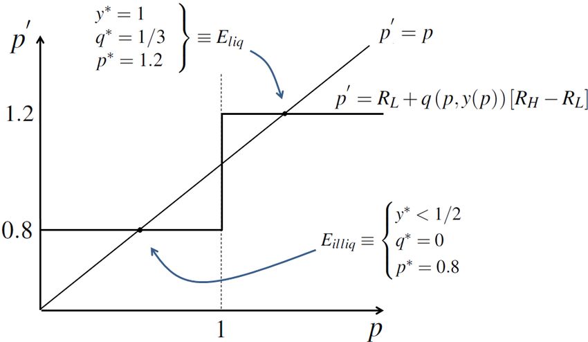
H. Example of a Self-fulfilling Liquidity Dry-up
Figure 1 illustrates that, in this economy, the same fundamentals (π, RH , RL ) might lead to multiple
equilibria that differ by their level of market liquidity.
[Figure 1 here]
7 Which is true in the interesting cases, that is, when p 6= 1.
0
8 Defined over [RL , RH ], the correspondence p (p) is nonempty-valued, convex-valued, and has a closed graph. The existence of
a fixed point is thus guaranteed by Kakutani’s theorem.
9In a first equilibrium (Eliq ), agents expect the market to be liquid (p > 1). Accordingly, they invest only
in the long-term asset. Given that they have no cash, agents H need to participate in the market to provide
for current consumption. This sustains a relatively high average quality (q∗ = 1/3) and ensures market
liquidity (p∗ = 1.2). However, if agents anticipate an illiquid market (p < 1), they initially choose to hoard.
Accordingly, agents H do not need to sell their assets, and the market breaks down: only lemons are for sale
(q∗ = 0). The market is thus illiquid (p∗ = RL ), which justifies the initial hoarding decision. Equilibrium
Eilliq is thus a self-fulfilling liquidity dry-up.
Both equilibria are locally stable in the sense that best responses to any small perturbation to the equi-
librium price would bring the price back to equilibrium. There are also equilibria corresponding to p = 1,
but they are unstable.9
I have assumed that agents L sell all their lemons when p = RL . Without this assumption, the quantity
they sell in the low-liquidity equilibrium is indeterminate (it is given by xL ∈ [0, y]), but the equilibrium
allocation of resources in unchanged. This allocation is unique given the initial investment decision and,
since there are no gains from trade, it is equivalent to a market freeze (which, strictly speaking, corresponds
to xL = 0). Given initial investment decisions, the high-liquidity equilibrium is also unique. It is a pooling
equilibrium (in prices, not in quantities) in the sense that agents L pretend they are of the H type and get the
same price, even though they sell larger quantities.10
The example depicted in Figure 1 is not an exception. In fact, a low-liquidity equilibrium always exists,
and if the long-term asset is sufficiently productive, a high-liquidity equilibrium exists too. Formally, for
each couple (π, RL ), there is a threshold for RH from which there are multiple equilibria.11
(2−π)
PROPOSITION 3 (Self-fulfilling liquidity dry-ups): If RH ≥ π − 2 (1−π)
π RL , both a low-liquidity equilib-
rium (i.e., with p∗ < 1) and a high-liquidity equilibrium (i.e., with p∗ > 1) exist. The low-liquidity equilib-
rium can thus be interpreted as a self-fulfilling liquidity dry-up.
Proof : straightforward.
III. Discussion
In this section, I first discuss the externality, whose identification is the main contribution of the paper.
Second, I provide a concrete application: namely, that imposing liquidity requirements on financial institu-
tions (a policy response to the recent financial crisis) may have unintended consequences. Third, I explain
how public liquidity insurance can prevent agents from coordinating on the Pareto-dominated equilibrium
of the model. Then, I highlight the relevant contexts to which the results apply, and I discuss the novel
9 There is a single symmetric equilibrium with p = 1, but since y(p) is not a singleton in that case, there is also an infinity of
asymmetric equilibria.
10 If quantity sold would be observable, a high-liquidity pooling equilibrium (in price and quantity) would exist under similar
conditions. The analysis could be done on the basis of this equilibrium. However, a separating equilibrium in which different types
trade different (and strictly positive) quantities at different prices might also exist.
11 Note that equilibrium multiplicity does not depend on the choice of the distribution of project quality, on the return to storage,
or on the specific form of the utility function. See the working paper version of the model for a proof of equilibrium multiplicity
under more general assumptions (Malherbe (2010)).
10empirical predictions. Finally, I highlight the key ingredients required to obtain the externality and relate
them to the main assumptions of the model.
A. The Externality
At date 1, the “true” value of an asset is Ri ∈ {RL , RH } per unit. Hence, a trade at a unit price of p 6= Ri
implies a transfer of value from the seller to the buyer (the transfer is negative if p > Ri ). At equilibrium, the
price adjusts so that the buyers break even on expectation. Therefore, an increase in the sale of good assets
increases the market price, which is beneficial to other sellers. This is the standard pecuniary externality
linked to adverse selection.
Whether an agent with a good asset chooses to trade, and therefore provides a positive externality, hinges
on his private valuation of this asset being lower than the market price. The key point in the model is that
his private valuation depends on his date-0 investment decision. The larger his position in the long-term
asset, the less cash he has at hand, and the more he needs to sell assets to cover current needs. Formally,
from Lemma 1, we have that xH (p, y), the quantity of asset sold when being of type H, is increasing in y.
Consequently, changes in y affect the expected quality of future sales.
The expected quality of an asset (the probability that it is a good one) sold by an agent who faces a price
p and has invested y is given by:
πxH (p, y)
qe (p, y) ≡ .
(1 − π)xL (p, y) + πxH (p, y)
The numerator is his expected sales of good assets, and the denominator is his expected total sales.12 A
∂ qe (p,y) 1
simple derivation establishes that ∂y ≥ 0, with strict inequality when y ≥ 1+p . An increase in y thus
improves the expected quality of future sales, which provides a nice intuition of how the externality works.
However, an increase in y also increases the quantity of lemons to be sold. To establish the externality, one
must look at the expected net effect.
Let me restrict the analysis to prices that are between the two equilibrium prices (including them), and
let me define t(p, y) as the expected transfer implied by future sales of an agent that invests y in the long-term
asset and faces a price p. That is:
t(p, y) ≡ πxH (p, y)(RH − p) + (1 − π)xL (p, y)(RL − p) .
An increase in t(p, y) increases the market price, which implies a positive externality. Similarly, a
decrease in t(p, y) implies a negative externality.
PROPOSITION 4 (Externality): Provided that y is not already too low, an increase in cash holding
h by an
i
∂t(p,y) 1
agent (i.e., a decrease in y) imposes a negative externality on other agents. That is, ∂y > 0, ∀y ∈ 1+p , 1 .
Proof : See Appendix
h A. i
1
Note that when y ∈ 1+p , 1 , xH (p, y) is strictly increasing in y (Lemma 1). The result is then obvious
12 In a symmetric equilibrium, qe (p, y) is equal to q(p, y(p)), the proportion of good assets in the market.
11when p = RL , and it can be easily generalized to the high-liquidity equilibrium price and to any price in
between.
Given the externality, it is not surprising that the high-liquidity equilibrium Pareto dominates the low-
liquidity one. Concretely, this is because: i) no resource is wasted in the storage technology; ii) Agents H
enjoy better consumption smoothing (these are the direct gains from trade); and iii) there is a cross-subsidy
from agents H to agents L, which is desirable from an ex-ante insurance perspective.
Note finally that the feedback effect that leads to equilibrium multiplicity comes from strategic comple-
mentarities13 in initial investment decisions. To see how they work and how they are linked to the externality,
consider the range of actions analyzed in Proposition 4. These actions decrease the market price. But a lower
market price makes the long-term asset less attractive (because a lower price decreases the option value to
sell at the interim date, without changing the cost of the investment) and thus makes increased cash hold-
ing more attractive. These actions therefore present strategic complementarities.14 This is another important
difference with the cash-in-the-market pricing literature, where cash holding decisions are typically strategic
substitutes.
B. Liquidity Requirement
In reaction to the recent crisis, regulators seem determined to require that financial institutions hold
more liquidity (the Basel Committee on Banking Supervision has recommended the imposition of a liquidity
coverage ratio (BCBS, 2011), and the Dodd-Frank Act stipulates that liquidity requirements should be taken
into account for setting prudential standards for systemically important financial institutions). While this
is a sensible thing to do to mitigate fire sale externalities, my results suggest that this may have adverse
unintended consequences when trades may reflect private information.
I present here a very simple exercise that illustrates this. Concretely, I consider a liquidity requirement
imposed by a regulator on date-0 investment decisions:
1 − y ≥ ρ, (9)
which simply means that a fraction ρ of the initial endowment should be kept in cash (i.e. should be stored).
The first implication is that it puts an upper bound on agents’ maturity mismatch, which can only reduce
their future needs to raise cash. Hence, it deters market participation for this motive and makes adverse
selection more severe.
PROPOSITION 5 (Unintended consequences): A liquidity requirement strictly reduces welfare at the high-
liquidity equilibrium and may even cause a liquidity dry-up.
Proof : see Appendix A.
First, observe that in a high-liquidity equilibrium, the liquidity buffer requirement (condition (9)) is
binding: when the market is liquid, storage is dominated and is kept at a minimum (y = 1 − ρ). By Lemma
13 In game theory, an action presents strategic complementarities if the incentive for an agent to take this action increases when
others take it.
14 Note that strategic complementarities are, however, not global: at a high initial level of cash holding, a further increase no
longer decreases the price and can even increase it. See Appendix B for further discussion.
121 (market participation), setting an upper bound to y can only deter agents H market participation: at a given
p, xH increases with y; it thus decreases with ρ. Average quality at the high-liquidity equilibrium (assuming
it still exists) is thus lower, and so is the price. Both types of agents are ex-post worse off because they are
forced to invest in a dominated technology, and this has no beneficial effect since the interim market price
is actually depressed. Second, because a higher ρ deters agents H market participation and depresses the
price, there is, for a given parameter set (RH ,RL, π), a ρ from which a market price superior or equal to 1
is not sustainable and market liquidity must dry up. In other words, an increase in ρ shrinks the parameter
region compatible with a high-liquidity equilibrium.
C. Coordination Failure and Public Liquidity Insurance
In this model, a self-fulfilling liquidity dry-up is a coordination failure: if agents expect others to hoard,
their best response is to hoard too, even though they know that a high-liquidity equilibrium is possible.
In this simple set-up, the coordination failure can, however, be easily prevented with public intervention.
For instance, the government can guarantee at date 0 a date-1 floor price of 1. In that case, cash becomes
a dominated asset, no-one hoards, and the only possible outcome is the Pareto-preferred equilibrium. This
intervention can be interpreted as a public liquidity insurance and is very similar in spirit to the demand
deposit insurance in Diamond and Dybvig (1983).
In more elaborate set-ups, however, the design of public intervention that aims at overcoming adverse
selection in financial markets is a complex issue. A first reason is that agents’ participation constraints
depend on expected public intervention (Tirole (2011b); Philippon and Skreta (2012)). But my results
suggest an additional layer of complexity: market participation also depends on cash holding positions,
which themselves depend on expected public intervention. One example is that the public liquidity insurance
mentioned above would only be effective if credibly announced ex ante. Once agents have decided to hoard,
guaranteeing a floor price is still feasible ex post, but it would no longer be a Pareto improvement. Hoarding
behavior may thus seriously impact the efficiency of public interventions such as those considered by Tirole
(2011b) and Philippon and Skreta (2012), and it would therefore be interesting to study this question in a
dynamic set-up that allows for ex-ante hoarding decisions.
D. Relevant Context and Empirical Predictions
The model applies to markets that may be subject to adverse selection on the sellers’ side. This can, for
example, be the case of markets for financial securities, such as common stocks or asset-backed securities,
or for corporate assets.15
The model first delivers empirical predictions related to the severity of adverse selection in contexts
where sellers’ “liquidity positions” are hard to assess by outsiders. Thus, these predictions are more likely to
apply when sellers are large and complex companies with opaque balance sheets rather than small companies
operating a single line of business (see Tirole (2011a), on the difficulty of assessing liquidity positions). A
15 See, for instance, Downing, Jaffee, and Wallace (2009) for evidence of adverse selection in the market for mortgage-backed
securities, and Rhodes-Kropf, Robinson, and Viswanathan (2005) for evidence of adverse selection in equity issuance linked to
corporate acquisition.
13worsening of adverse selection in a given market is characterized by lower prices, lower volumes, and lower
average quality of the assets that are traded (compared to those that are not) and by higher incentives to
invest in costly information acquisition about these assets.
PREDICTION 1: Adverse selection intensifies in periods of high cash holding.
The unusual and widespread hoarding behavior that has been observed in the aftermath of the recent
financial crisis makes it an interesting context for testing this prediction.16 A case in point could be asset-
backed securities. Indeed, while their design is supposed to alleviate adverse selection (DeMarzo and Duffie
(1999); DeMarzo (2005)), these securities had largely become “toxic” in the fall of 2008, a phenomenon
widely associated with adverse selection (Morris and Shin (2012); Tirole (2011b)). However, the econ-
omy had also entered a recession that was likely to be severe. Bad news about fundamentals increases the
information sensitivity of debt-like assets and makes them more prone to adverse selection (Gorton and
Pennacchi (1995); Dang, Gorton, and Holmström (2009)). But this second channel is not incompatible with
the cash-holding one. In fact, the two effects are likely to reinforce each other and would probably be hard
to disentangle during this period. Still, issuance in securitization markets has, by and large, not recovered
(Gorton and Metrick, 2011), while macroeconomic fundamentals have arguably improved (at least in the
US). This provides support for the economic significance of the cash-holding channel.
PREDICTION 2: When sellers’ cash needs decrease (increase), or when other sources of cash become more
easily (less easily) available to them, adverse selection intensifies (abates).
This prediction relates directly to my discussion above on liquidity requirements. It applies, for instance,
to markets where financial institutions are natural sellers/issuers. An example of changing refinancing con-
ditions could be an increase in the range of collateral eligible for borrowing at the central bank or a change
in the class of institutions that can access central bank lending. Such changes have been made during the re-
cent crisis to ease the short-term funding of financial institutions. The model suggests that they may actually
have worsened adverse selection in other markets (such as those for asset-backed securities, for example).
The same must be said of the ECB’s recent launch of long term refinancing operations (LTRO), since it
implies a protracted period of easy refinancing for financial institutions in the euro area.
PREDICTION 3: Sellers of assets that are prone to adverse selection are relatively more likely to release
information on cash needs and to report reasons for selling that are allegedly unrelated to the quality of the
assets they sell.
Divesting firms often publicly announce that the assets they sell are “non-core” (or “non-strategic”)
and/or that the divestiture is driven by cash needs. Informing investors about corporate strategy could be
the purpose of such announcements, but it may also be an attempt to alleviate suspicions of an opportunistic
sale.17 There is a large body of literature studying the impact of divestiture on firm performance. Some
16 From August 2007, UK banks have increased their liquidity buffers by 30% (Acharya and Merrouche (2012)); from September
2008, there has been a dramatic increase in the excess reserves of European banks (Heider, Hoerova, and Holthausen, 2010; Pisani-
Ferry and Wolff (2012)), and of US major deposit institutions. Keister and McAndrews (2009), however, point out that a substantial
part of the increase could be due to factors other than hoarding.
17 After all, as pointed by Tirole (2011a), this is not so different from having ads for used cars or houses mentioning exogenous
14papers have studied the motives for selling (Lang, Poulsen, and Stulz (1995), Hite, Owers, and Rogers
(1987), and John and Ofek (1995), for example) but, to the best of my knowledge, the interaction between
alleged selling motives and adverse selection has been rather overlooked. If such communication arises
more often when the assets for sale are prone to adverse selection, and/or is associated with smaller lemons
discounts, this would provide support for the model.
The model also delivers predictions related to contexts where the seller’s cash position is easier to assess
by outsiders. The first is the counterpart of Prediction 3.
PREDICTION 4: Cash-rich firms are relatively more likely to invest in costly disclosure of information on
the quality of the assets they sell (pay certification fees, for instance) and to report reasons for selling that
are allegedly unrelated to their quality.
When selling assets equally prone to adverse selection, firms with more cash at hand are indeed more
likely to try to alleviate suspicions that sales are driven by private information.
Proposition 4 implies that the average quality of sold assets is decreasing with initial cash holdings. The
model therefore predicts that when buyers observe large cash holdings by a seller, they should assign high
probability to the sale being driven by private information, and they should offer a low price. Accordingly:
PREDICTION 5: Cash-rich firms are likely to face relatively larger lemons discounts.
Empirical studies on the relationship between cash positions and lemons discounts are scarce. However,
Gao (2011) finds empirical evidence for an adverse selection effect of corporate cash reserve in the context
of acquisitions that are financed by stocks. In particular, he finds that announcement returns are lower for
bidders with higher excess cash reserves, which is consistent with my prediction.
If they face larger lemons discounts, cash-rich firms should be more reluctant to sell information-
sensitive assets. Hence:
PREDICTION 6: Cash-rich firms are relatively less likely to sell assets that are prone to adverse selection.
This prediction has to be contrasted with the prediction of Myers and Majluf (1984) that a larger financial
slack makes a firm more likely to issue equity. The difference comes mostly from their assumption of a fixed-
size investment opportunity. In their paper, more financial slack means that less capital needs to be raised
to seize the opportunity. Since the net present value of the project is constant, the marginal return to raising
capital is increasing in financial slack. In my model, in contrast, the marginal utility of cash obtained from
the sale decreases with the cash that was already available.
E. Key Features of the Model
This paper makes the point that cash holding can impose a negative externality as it worsens adverse
selection in markets for long-term assets. While the point is made in the context of a simple and very stylized
model, it applies quite generally to contexts where cash positions are not easily observable. In these cases,
one should expect it to be relevant in most situations where both private information and a need to raise cash
are potential motives for selling assets.
reasons for selling (move abroad, family extension, etc.).
15If cash positions were observable in the model, an increase in cash holdings by an agent would still
decrease the average quality of his future sale but would not impose an externality on others because the
market perception of their trading motive could be directly based on their own cash position. The combi-
nation of the two motives for selling is the other key feature of the model. Individually, these motives are
of course quite common. To illustrate that they do not hinge on very specific assumptions, I identify where
they come from in the model and I provide examples of alternate relevant situations.
First, to have private information as a potential selling motive, I simply assume that agents privately
observe their project quality at the beginning of date 1, and I rule out contracts that would make private
information irrelevant at that date. The underlying specific restrictions are not important. What really
matters is that sellers have relevant private information when the market opens. Holmström and Tirole
(2011) confirm this in a version of the model where agents can trade at date 0 but are then already privately
informed.
Second, the potential need to raise cash comes, in the model, from agents deriving utility from date-1
consumption. Any other reasons why cash would be valuable at date 1 (an investment opportunity or a
refinancing need, for instance) would also yield such a selling motive.
Finally, note that it is essential that cash holding attenuates the need for cash. It may seem trivial, but
cash needs should be endogenous. But this is, for instance, usually not the case in models that, in the
tradition of Diamond and Dybvig (1983), assume that a fraction of agents are hit by a shock that gives
them an absolute preference for cash.18 By contrast, in my model, the decreasing marginal utility of date-1
consumption ensures that the need to raise cash decreases with cash holding. This would also be the case
if the need for cash would come from a (possibly random) investment opportunity with a concave return
function (with some strict concavity), but not in the case of an investment opportunity with linear return and
infinite possible scale (as is sometimes implicitly assumed in the security design literature).19
IV. Conclusion
I have presented a model in which cash holding imposes a negative externality. This model sheds light
on a new channel by which hoarding behavior may impair the efficient allocation of resources.
By and large, the results contrast with those of the cash-in-the-market/fire-sale literature, in which liq-
uidity holding imposes a positive externality. Whether private agents tend to hold too much or too little
liquidity thus depend on the nature of the underlying friction, that is, whether there is an adverse selection or
a moral hazard problem. The respective policy implications are opposite. In particular, my model suggests
that imposing liquidity requirements on financial institutions, a policy that mitigates fire-sale externalities,
is likely to have adverse unintended consequences in markets prone to adverse selection.
As a matter of fact, the regulatory response to the recent crisis suggests that fire sales are seen as most
relevant. However, given the current amount of excess reserves of financial institutions in Europe and in
18 This special case usually yields corner solutions for sale decisions, in which case the severity of adverse selection is likely to
be uniquely determined by the fraction of agents hit by the shock. See Parlour and Plantin (2008) for an example.
19 See DeMarzo and Duffie (1999), for instance.
16the US, it is difficult to argue that private agents always tend to hold too little liquidity and that hoarding
behavior is only a remote theoretical possibility. Regulators should therefore not overlook the mechanism
highlighted in this paper.
17Appendix A. Proofs
Proof of Proposition 1:
i) The case where p > 1 is trivial as cash holding is a dominated means to transfer resource to date 1 and
date 2. Thus y(p) | p>1 = 1.
ii) When p = 1, to hold cash is equivalent to invest and then sell, and it is straightforward to show that
RH
the optimal contingent consumption plan corresponds to c2H = 2 , and c1H = c1L = c2L = 21 . This plan is
feasible if and only if y ∈ 21 , 1 .
1+y(p−1)
iii) Consider now p < 1. From equation (4), I have: UL (p < 1, y) = 2 ln 2 and, from equation
(5),
1+y(RH −1) 1
2 ln 2 ; y ≤ 1+R H
UH (p < 1, y) = ln(1 − y) + ln(yRH ) 1 1 (10)
; 1+RH ≤ y ≤ 1+p
ln 1+y(p−1) + ln 1+y(p−1) RH
1
; 1+p ≤y
2 2 p
0
h i 0
Letting Ui ≡ ∂U∂y
0
|i be the marginal utility of y conditionally on being in the state i, I have: UL < 0, ∀y,
0 0 0
and: UH T 0 if y S 21 . Therefore (1 − π)UL + πUL is always strictly negative for all y ≥ 21 . Hence, it can
only be null for a y ∈ 0, 21 , and it must be the case that y(p) | p 0, ∀y ∈ 1+p , 1 and p ∈ RL , pliq , where
π
pliq ≡ RL + 2−π (RH − RL ) is the price at the high-liquidity equilibrium.
1
When y ≥ 1+p , from equation (5), I have:
∂t(p, y) p+1
= π(RH − p) + (1 − π)(RL − p)
∂y 2p
∂t(p,y)
First, note that ∂y is decreasing in p. Thus, I can focus on p = pliq since it is the most unfavorable
1
case. Since buyers break even on expectation at equilibrium, I have: t(pliq , 1) = 0. But, when y = 1+pliq , I
1 1 (1−π)(RL −pliq ) 1
have xH (pliq , 1+p liq
) = 0. This implies that t(pliq , 1+p liq
)= 1+pliq < 0. Since 1+p liq
< 1, and ∂t(p,y)
∂y
h i
∂t(p,y) 1
does not depend on y, it must thus be the case that ∂ y > 0, ∀y ∈ 1+pliq , 1 , which establishes the result.
0
Proof of Proposition 5: First, define p (p, ρ) ≡ RL + q (p, y(p, ρ)) [RH − RL ], the implied price corre-
00 0
spondence for a given ρ; let p (ρ) denote the largest fixed point that solves p (p, ρ) = p; and show that, if
00
it exists p (ρ) is strictly decreasing in ρ, for p > 1.
A direct adaptation of Proposition 1 (optimal investment) gives thatnconstraint (9)ois binding when p > 1.
Hence, at the optimal investment level, xH (p, y) = xH (p, 1 − ρ) = max 0; 1−ρ ρ
2 − 2p . Since it is decreasing
in ρ, the resulting average quality q(p, 1−ρ) is decreasing in ρ too, and it is easy to check that it is increasing
in p. Therefore, considering two different requirements ρlow < ρhigh , the price corresponding to the largest
00
fixed point under ρlow (it is denoted p (ρlow )) is larger than the price it would imply under ρhigh , that is:
0 00 00 00
p (p (ρlow ), ρhigh ) < p (ρlow ). Hence, p (ρlow ) cannot be a fixed point under ρhigh . Since q(p, 1 − ρ) is
1800
decreasing in ρ for any p, and, by definition, p (ρlow ) is the largest fixed point under ρlow , there cannot exist
00 00 00
a fixed point p (ρhigh ) such that p (ρhigh ) ≥ p (ρlow ).
00 00
Then, note that there is a ρ < 1, such that xH (p (0), 1 − ρ) = 0. Since p (ρ) is strictly decreasing for
00
p > 1 and xH (p, y) decreases with p, there is a ρ < 1 from which xH (p, 1 − ρ) = 0, for any p ≤ p (0), which
00
is inconsistent with the existence of a high liquidity equilibrium. Then, since p (ρ) is strictly decreasing for
00
p > 1, there exist a ρ̂ such that p (ρ) = RL , ∀ρ > ρ̂.
Finally, if the high-liquidity equilibrium still exists under the liquidity requirement, that both types of
agents are strictly worse off with a liquidity requirement is a direct consequence of the externality. Since p
is lower with the requirement, agents L, who sell everything, are strictly worse off. Agents H are strictly
worse off too because mandatory cash holding wastes resources, which strictly shrinks their budget set, and
because the price of date-1 consumption becomes higher (since p is lower).
Appendix B. Lack of Global Strategic Complementarities
In this appendix, I show that increasing cash holdings when they are already high presents strategic
substitutabilities, and I argue that it precludes the use of standard equilibrium selection techniques.
B1. Strategic Substitutabilities
p
I show that when 1 − y ≥ 1+p , increasing cash holdings further increases the expected transfer and,
hence, the market price. Since an increase in price decreases incentives to increase cash holdings, this
establishes the strategic substitutabilities.
p 1
Since 1 − y ≥ 1+p corresponds to y < 1+p , it implies that xH (p, y) = 0. In that case,
∂t(p, y)
= (1 − π)(RL − p) ≤ 0 .
∂y
There are two relevant cases to consider: either p = RL (which is the case at the low-liquidity equilib-
rium) or p > RL (which is the case at the high-liquidity equilibrium but can also happen out of equilibrium).
∂t(p,y)
The interesting case is the latter, because ∂y < 0 implies that an increase in cash holdings (a decrease
in y) imposes a positive pecuniary externality. An agent who increases cash holdings decreases the quantity
1
of long-term assets he invests in. If these turn out to be good, he does not sell them (because y < 1+p );
if they turn out to be lemons, he sells them. But the quantity of lemons he sells has decreased. Thus the
expected transfer increases (it is negative but decreases in absolute value). This establishes the strategic
substitutabilities. When p = RL , there are only lemons in the market, and an increase in cash holdings does
not affect the price.
B2. Implications for Equilibrium Selection
In games of strategic complementarities, while multiple equilibria are typical, they are generally not
robust to a slight departure from the assumption that agents share a common knowledge of the economic
environment. For instance, under global strategic complementarities one can generally use equilibrium se-
lection techniques based on the iterative deletion of dominated strategies, such as global games (Carlsson
19and van Damme (1993); Morris and Shin (2004); Frankel, Morris, and Pauzner (2003); Vives (2005)). When
they concern actions that are outside the relevant range of possible actions, the presence of strategic substi-
tutabilities does not preclude equilibrium uniqueness under incomplete information (Goldstein and Pauzner
(2005); Mason and Valentinyi (2010); Bueno de Mesquita (2011)). However, the strategic substitutabilities
present in my model concern the relevant range of action. Technically, it can be shown that they imply
that best responses to monotonic strategies are not always monotonic, which rules out the single-crossing
conditions for uniqueness exploited in Goldstein and Pauzner (2005), Mason and Valentinyi (2010), and
Bueno de Mesquita (2011).
20You can also read