Sentience and the Origins of Consciousness: From Cartesian Duality to Markovian Monism - University College London
←
→
Page content transcription
If your browser does not render page correctly, please read the page content below
entropy
Article
Sentience and the Origins of Consciousness:
From Cartesian Duality to Markovian Monism
Karl J. Friston 1, *, Wanja Wiese 2, *         and J. Allan Hobson 3, *
 1    The Wellcome Centre for Human Neuroimaging, Institute of Neurology, Queen Square,
      London WC1N 3AR, UK
 2    Department of Philosophy, Johannes Gutenberg University Mainz, Jakob-Welder-Weg 18,
      55128 Mainz, Germany
 3    Division of Sleep Medicine, Harvard Medical School, 74 Fenwood Road, Boston, MA 02115, USA
 *    Correspondence: k.friston@ucl.ac.uk (K.J.F.); wawiese@uni-mainz.de (W.W.);
      allan_hobson@hms.harvard.edu (J.A.H.)

 Received: 4 February 2020; Accepted: 16 April 2020; Published: 30 April 2020

 Abstract: This essay addresses Cartesian duality and how its implicit dialectic might be repaired
 using physics and information theory. Our agenda is to describe a key distinction in the physical
 sciences that may provide a foundation for the distinction between mind and matter, and between
 sentient and intentional systems. From this perspective, it becomes tenable to talk about the physics of
 sentience and ‘forces’ that underwrite our beliefs (in the sense of probability distributions represented
 by our internal states), which may ground our mental states and consciousness. We will refer to
 this view as Markovian monism, which entails two claims: (1) fundamentally, there is only one type
 of thing and only one type of irreducible property (hence monism). (2) All systems possessing a
 Markov blanket have properties that are relevant for understanding the mind and consciousness:
 if such systems have mental properties, then they have them partly by virtue of possessing a Markov
 blanket (hence Markovian). Markovian monism rests upon the information geometry of random
 dynamic systems. In brief, the information geometry induced in any system—whose internal states
 can be distinguished from external states—must acquire a dual aspect. This dual aspect concerns
 the (intrinsic) information geometry of the probabilistic evolution of internal states and a separate
 (extrinsic) information geometry of probabilistic beliefs about external states that are parameterised by
 internal states. We call these intrinsic (i.e., mechanical, or state-based) and extrinsic (i.e., Markovian,
 or belief-based) information geometries, respectively. Although these mathematical notions may
 sound complicated, they are fairly straightforward to handle, and may offer a means through which
 to frame the origins of consciousness.

 Keywords: consciousness; information geometry; Markovian monism

1. Introduction
     The aim of this essay is to emphasise a couple of key technical distinctions that seem especially
prescient for an understanding of the beliefs and intentions that underpin pre-theoretical notions of
consciousness. What follows is an attempt to describe constructs from information theory and physics
that place certain constraints on the dynamics of self-organising creatures, such as ourselves. These
constraints lend themselves to an easy interpretation in terms of beliefs and intentions; provided
one defines their meaning carefully in relation to the mathematical objects at hand. The benefit of
articulating a calculus of beliefs (and intentions) from first principles has yet to be demonstrated;
however, just having a calculus of this sort may provide useful perspectives on current philosophical
debates. Furthermore, trying to articulate pre-theoretical notions in terms of maths should, in principle,

Entropy 2020, 22, 516; doi:10.3390/e22050516                                    www.mdpi.com/journal/entropy
Entropy 2020, 22, 516                                                                                                    2 of 31

expand the scope of dialogue in this area. To illustrate this, we will try to license talk about physical
forces causing beliefs in a non-mysterious way—a way that clearly identifies systems or artefacts that
are and are not equipped with processes that can ground mental capacities and consciousness.
      To make a coherent argument along these lines, it will be necessary to introduce a few technical
concepts. The formal basis of the arguments in this—more philosophical—treatment of sentience and
physics can be found in [1]. The current paper starts were Friston (ibid.) stops; namely, to examine
the philosophical implications of Markov blankets and the ensuing Bayesian mechanics. For readers
who are more technically minded, the derivations and explanations of the equations in this paper
can be found in [1] (using the same notation). We have attempted to unpack the derivations for
non-mathematical readers but will retain key technical terms, so that the lineage of what follows can
be read clearly. To avoid cluttering the narrative with definitions, a glossary of terms and expressions
is provided at the end of the paper. In brief, we first establish the basic setup used to describe
physical systems that evince the phenomenology necessary to accommodate pre-theoretical notions of
consciousness. This will involve the introduction of Markov blankets and the distinction between the
internal and external states of a system or creature.
      Having established the distinction between external and internal states, we introduce the notion of
information length and information geometry. This is the first key move in the theoretical analysis on
offer. Crucially, information geometry allows us to establish a calculus of beliefs in terms of probability
distributions. This calculus enables a distinction to be made between the probability distribution about
things and the probability distribution of things. This distinction is then treated as one way of describing
an account that (literally) maps belief states onto physical states; here, beliefs about external states that
are parameterised, represented, encoded or coherent with internal states. We shall call the ensuing
view Markovian monism because it is predicated on the existence of a Markov blanket.
      This brings us to a modest representationalism1 , which allows one to talk about flows, energy
gradients and forces that shape the dynamics of internal states and, necessarily, the beliefs they
parameterise. The next section considers the nature of these beliefs and, in particular, beliefs about
how internal states couple to external states; namely, beliefs about action upon the world ‘out there’.
To do this formally, we have to look at two distinct ways of describing the dynamics and introduce
the notion of trajectories via the path integral formulation. Having done this, we can then associate
intentions with beliefs about action—that, in turn, depend upon beliefs about the consequences of
action. At this point, we can make a distinction between systems that have a rudimentary information
geometry of a reflexive, instantaneous sort—and systems that hold beliefs about the future. It is this
quantitative distinction that may provide a spectrum of intentional or agential systems, ranging from
protozoa to people. We conclude with a brief discussion of related formulations—and how the central
role of sentience, observation, measurement, or inference opens the door for further developments
of a sentient physics. In particular, we will discuss how Markovian monism can be interpreted in
terms of existing theories regarding the relationship between mind and matter, such as neutral monism
and panprotopsychism.

1   The important point is that such systems can be described ‘as if’ they represent probability distributions. More substantial
    representationalist accounts can be built on this foundation, see Section 13.
Entropy 2020, 22, 516                                                                                  3 of 31

      The primary target of this paper is sentience. Our use of the word “sentience” here is in the
sense of “responsive to sensory impressions”. It is not used in the philosophy of mind sense; namely,
the capacity to perceive or experience subjectively, i.e., phenomenal consciousness, or having ‘qualia’.
Sentience here, simply implies the existence of a non-empty subset of systemic states; namely, sensory
states. In virtue of the conditional dependencies that define this subset (i.e., the Markov blanket
partition), the internal states are necessarily ‘responsive to’ sensory states and thus the dictionary
definition is fulfilled. The deeper philosophical issue of sentience speaks to the hard problem of tying
down quantitative experience or subjective experience within the information geometry afforded by
the Markov blanket construction. We will return to this below.
      While most of this paper deals with sentience in the sense just specified, it may shed light on
the origins of consciousness. First, applying the concept of subjective, phenomenal consciousness to
a system trivially presupposes that this system can be described from two perspectives (i.e., from a
third- and from a first-person perspective). Second, the minimal form of goal-directedness and ‘as
if’ intentionality—that one can ascribe to sentient systems—provide conceptual building blocks that
ground more high-level concepts, such as physical computation, intentionality, and representation,
which may be useful to understand the evolutionary transition from non-conscious to conscious
organisms, and thereby illuminate the origins of consciousness.

2. Markov Blankets and Self-Organisation
       Before we can talk about anything, we have to consider what distinguishes a ‘thing’ from
everything else. Mathematically, this requires the existence of a particular partition of all states a system
could be in into external, (Markov) blanket and internal states. A Markov blanket comprises a set of
states that renders states internal to the blanket conditionally independent of external states. The term
was originally coined by Pearl in the context of Bayesian networks [2]. For a Bayesian network (i.e.,
a directed acyclic graphical model) the Markov blanket comprises the parents, children, and parents
of the children of a state or node. For a Markov random field (i.e., an undirected graphical model),
the Markov blanket comprises the parents and children, i.e., its neighbours. For a dependency network
(i.e., a directed cyclic graphical model) the Markov blanket comprises just the parents. For treatments of
Markov blankets in the life sciences, please see [3–8]. The three-way partition induced by the Markov
blanket enables one to distinguish internal and external states via their conditional independence,
given blanket states. The blanket states themselves can be further partitioned into sensory and active
states, where sensory states are not influenced by internal states and active states are not influenced by
external states [9]. Note that all we have done here is to stipulatively define a ‘thing’ in terms of its
internal states (and Markov blanket) in terms of what does not influence what. The requisite absence of
specific influences are precisely those described above; namely, internal states and external states only
influence each other via the Markov blanket, while sensory states are not influenced by internal states,
a similar relationship is true for active and external states. A key insight here is that structure emerges
from influences that are not there, much like a sculpture emerges from the material removed. There are
lots of interesting implications of defining things in terms of Markov blankets (please see Figure 1 for a
couple of intuitive examples); however, we will place the notion of a Markov blanket to one side for
the moment and consider how systemic states behave in general. After this, we will then consider the
implications of this generic behaviour, when there is a Markov blanket play.
Entropy 2020, 22, 516 4 of 31
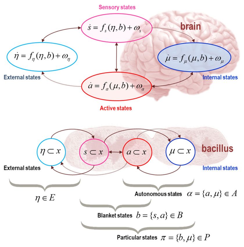
Figure 1. (Markov blankets): This schematic illustrates the partition of systemic states into internal
states (blue) and hidden or external states (cyan) that are separated by a Markov blanket—comprising
sensory (magenta) and active states (red). The upper panel shows this partition as it would be applied
to action and perception in the brain. The ensuing self-organisation of internal states then corresponds
to perception, while action couples brain states back to external states. The lower panel shows the same
dependencies but rearranged so that the internal states are associated with the intracellular states of a
Bacillus, while the sensory states become the surface states or cell membrane overlying active states
(e.g., the actin filaments of the cytoskeleton).
3. The Langevin Formalism and Density Dynamics
Starting from first principles, if we assume that a system exists, in the sense that it has measurable
characteristics over some nontrivial period of time,2 then we can express its evolution in terms of a
random dynamical system. This just means that the system can be described in terms of changes in
states over time that are subject to some random fluctuations:
x(τ) = f (x, τ) + ω. (1)
This is a completely general specification of (Langevin) dynamics that underwrites nearly
all of physics [10–12]. In brief, the dynamics in (1) can be described in terms of two equivalent
formulations—the dynamics of the accompanying probability density over the states and the path
integral formulation.3
2 In the sense that anything just is a Markov blanket, the relevant timescale is the duration over which the thing exists.
Generally, smaller things last for short periods of time and bigger things last longer. This is a necessary consequence of
composing Markov blankets of Markov blankets (i.e., things of things). In terms of sentient systems, the relevant time scale
is the time over which a sentient system persists (e.g., the duration of being a sentient person).
3 In turn, this leads to quantum, statistical and classical mechanics, which can be regarded as special cases of density
dynamics under certain assumptions. For example, when the system attains nonequilibrium steady-state, the solution to
the density dynamics (i.e., Fokker Planck equation) becomes the solution to the Schrödinger equation that underwrites
quantum electrodynamics. When random fluctuations become negligible (in large systems), we move from the dissipative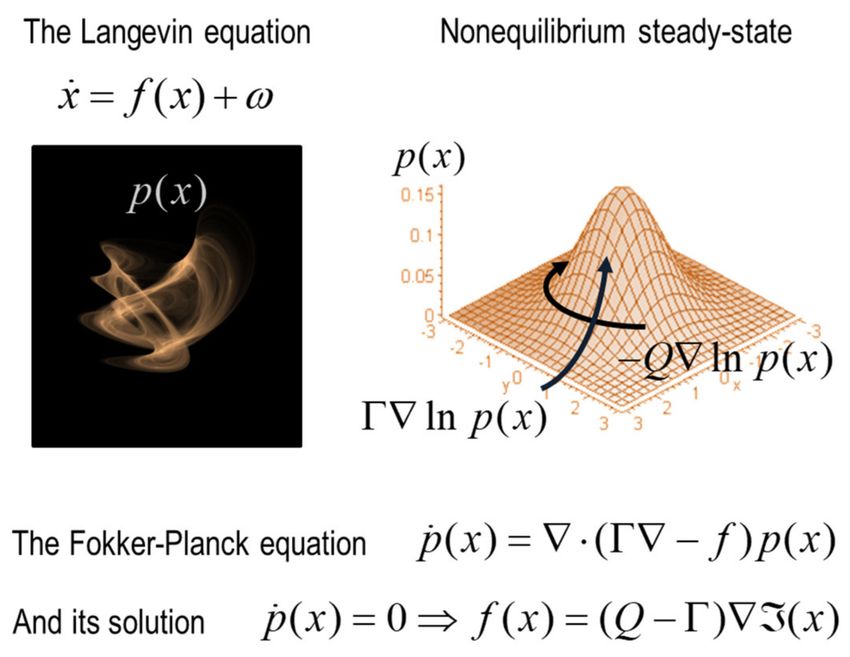
Entropy 2020, 22, 516                                                                                                       5 of 31

      We will be interested in systems that have measurable characteristics, which means that they must
converge to some attracting set or manifold, known as a random or pullback attractor [13].4 After a
sufficient period of time, as the system evolves, it will trace out a trajectory—in state space—that
circulates, usually in a highly itinerant fashion, on the attracting manifold. This means that if we
observe the system at random, there is a certain probability of finding it in a particular state. This is
known as the nonequilibrium steady-state density [12].
      It is natural to ask whether a single attracting manifold is an appropriate construct to describe a
system or creature over its lifetime; especially when certain ‘life-cycles’ have distinct developmental
stages or indeed feature metamorphosis. From the perspective of the current argument, it helps to
appreciate that the attracting manifold is itself a random set.5 In other words, a particle or person is
never ‘off’ their manifold—they just occupy states that are more or less likely, given the kind of thing
they are (i.e., something’s characteristic states are an attracting set of states that it is likely to occupy).
Technically, this peripatetic itinerancy corresponds to stochastic chaos, where excursions from the
attracting set—driven by random fluctuations—are an integral aspect of the dynamics. These excursions
are repaired through the flow that counters the effects of random fluctuations and underwrites the
information geometry of self-organisation. This formulation can, in principle, accommodate slow
changes to the attracting set—and implicit Markov blanket—that may require the notion of wandering
sets [14].
      The reason that this is interesting is that one can use standard descriptions of density dynamics to
express the flow of states as a gradient flow on something called self-information or surprisal [15–18].
Without going into details, this is the steady-state solution to the Fokker Planck equation [19–23].
This equation says that, on average, the states of any system with an attracting set must conform to a
gradient flow on surprisal; namely, the negative logarithm of the probability density at nonequilibrium
steady state [24,25].
                                            f (x) = (Q − Γ) · ∇I(x)
                                                                                                            (2)
                                            I(x) = − ln p(x)
     This is the solution to the Fokker-Planck equation when the system has attained nonequilibrium
steady-state. It says that the average flow of systemic states has two parts. The first (gradient)
component involves surprisal gradients, while the second circulates on iso-probability contours.
The gradient flow effectively counters the dispersion due to random fluctuations, such that the
probability density does not change over time. See Figure 2 for an intuitive illustration of this solution.
     The key move now is to put the Markov blanket back in play. The above equation holds
(nontrivially) for the internal, blanket, and external states, where we can drop the appropriate states
from the gradient flows, according to the specification of the Markov blanket in Figure 1. In particular,
if we just focus on internal and active states—which we will refer to as autonomous states—we have the
following flows6 (see p. 17 and pp. 20,21 in [1]).

                                               fα (π) = (Qαα − Γαα )∇α I(π)
                                                         α = a, µ

                                                                                                                               (3)
                                                         π = {s, α}

    thermodynamics to conservative classical mechanics. A technical treatment along these lines can be found in [1] with
    worked (numerical) examples.
4   Technically, Equation (1) only holds on the attracting set. However, this does not mean the dynamics collapse to a single
    point. The attracting manifold would usually support stochastic chaos and dynamical itinerancy—that may look like a
    succession of transients.
5   Note that the attracting set is in play throughout the ‘lifetime’ of any ‘thing’ because, by definition, a ‘thing’ has to be at
    nonequilibrium steady-state. This follows because the Markov blanket is a partition of states at nonequilibrium steady-state.
6   Note that as in (2) Qαα and Γαα denote antisymmetric and leading diagonal matrices, respectively.
Entropy 2020, 22, 516 6 of 31
Figure 2. (density dynamics and pullback attractors): This figure illustrates the fundaments of density or
ensemble dynamics in random dynamical systems—of the sort described by the Langevin equation.
The left panel pictures some arbitrary random attractor (a.k.a., a pullback attractor) that can be thought
of in two ways: first, it can be considered as the trajectory of (two) systemic states as they evolve
over time. For example, these two states could be the depolarisation and current of a nerve cell,
over several minutes. At a larger timescale, this trajectory could reflect your daily routine, getting
up in the morning, having a cup of coffee, going to work and so on. It could also represent the slow
fluctuations in two meteorological states over the period of a year. The key aspect of this trajectory is
that it will—after itinerant wandering and a sufficient period of time—revisit particular regimes of
state space. These states constitute the attracting set or pullback attractor. The second interpretation
is of a probability density over the states that the system will be found in, when sampled at random.
The evolution of the probability density is described by the Fokker-Planck equation. Crucially, when any
system has attained nonequilibrium steady state, we know that this density does not change with
time. This affords the solution to the Fokker-Planck equation—a solution that means that there is a
lawful relationship between the flow of states at any point in state space and the probability density.
This solution expresses the flow in terms of gradients of log density or surprisal and the amplitude of
random fluctuations. In turn, the nonequilibrium steady-state solution can always be expressed, via the
Helmholtz decomposition, in terms of two orthogonal components. One component is a gradient flow
that rebuilds probability gradients in a way that is exactly countered by the dispersion of states due
to random fluctuations. The other component is a solenoidal or divergence-free flow that circulates
on isoprobability contours. These two components are shown in the schematic on the right, in terms
of a curl-free gradient flow—that depends only on the amplitude of random fluctuations Γ– and a
divergence-free solenoidal flow—that depends upon an antisymmetric matrix Q. This example shows
the flow around the peak of a probability density, with a Gaussian form. Please see [1,25] for details.
This means anything that can be measured (i.e., a system with a Markov blanket and attracting
set) must possess the above gradient flows. In turn, this means that internal and active states will
look as if they are trying to minimise exactly the same quantity; namely, the surprisal of states that
constitute the thing, particle, or creature. These are the internal states and their Markov blanket; i.e.,
particular states.7 This means that anything that exists must, in some sense, be self-evidencing [37].
7 In itself, this is remarkable, in the sense that it captures the essence of many descriptions of adaptive behaviour, ranging from
expected utility theory in economics [26–28] through to synergetics and self-organisation [21,29]. See Figure 3. To see how
these descriptions follow from the gradient flows in (3), we only have to note that the mechanics of internal and active states
can be regarded as perception and action, where both are in the service of minimising a particular surprisal. This surprisal
can be regarded as a cost function from the point of view of engineering and behavioural psychology [30–32]. From the
perspective of information theory, surprisal corresponds to self-information, leading to notions such as the principle of
minimum redundancy or maximum efficiency [33]. The average value of surprisal is entropy [17]. This means that anything
that exists will—appear to—minimise the entropy of its particular states over time [29,34]. In other words, it will appear toEntropy 2020, 22, 516 7 of 31
Figure 3. (Markov blankets and other formulations): This schematic illustrates the various interpretations
of a gradient flow on surprisal. Recall that the existence of a Markov blanket implies a certain lack
of influences among internal, blanket, and external states. At nonequilibrium steady-state, these
independencies have an important consequence; internal and active states are the only states that
are not influenced by external states, which means their dynamics (i.e., perception and action) are a
function of, and only of, particular states; i.e., a particular surprisal.8 This surprisal has a number of
interesting interpretations. Given it is the negative log probability of finding a particle or creature in a
particular state, minimising particular surprisal corresponds to maximising the value of a particle’s
state. This interpretation is licensed by the fact that the states with a high probability are, by definition,
attracting states. On this view, one can then spin-off an interpretation in terms of reinforcement
learning [30], optimal control theory [31] and, in economics, expected utility theory [39]. Indeed,
any scheme predicated on the optimisation of some objective function can now be cast in terms of
minimising a particular surprisal—in terms of perception and action (i.e., the flow of internal and
active states). The minimisation of particular surprisal leads to a series of influential accounts of
neuronal dynamics; including the principle of maximum mutual information [40,41], the principles
of minimum redundancy and maximum efficiency [33] and—as we will see later—the free energy
principle [42]. Crucially, the average or expected surprisal (over time or particular states of being)
corresponds to entropy. This means that action and perception look as if they are minimising a
particular entropy. The implicit resistance to the second law of thermodynamics leads us to theories of
self-organisation, such as synergetics in physics [29,43,44] or homoeostasis in physiology [35,45,46].
Finally, the probability of any particular states given a Markov blanket (m) is, on a statistical view,
model evidence [18,47]. This means that all the above formulations are internally consistent with
things like the Bayesian brain hypothesis, evidence accumulation and predictive coding; most of which
inherit from Helmholtz’s motion of unconscious inference [48], later unpacked in terms of perception
as hypothesis testing in 20th century psychology [49] and machine learning [50]. In short, the very
existence of something leads in the natural way to a whole series of optimisation frameworks in the
physical and life sciences that lends each a construct validity in relation to the others.
resist the second law of thermodynamics (which is again remarkable, because we are dealing with open systems that are far
from equilibrium). From the point of view of a physiologist, this is nothing more than a generalised homoeostasis [35].
Finally, from the point of view of a statistician, the negative surprisal would look exactly the same as Bayesian model
evidence [36].Entropy 2020, 22, 516 8 of 31
4. Bayesian Mechanics
Thus, if we can describe anything as self-evidencing—in the sense of possessing a dynamics
that tries to minimise a particular surprisal—or maximise a particular model evidence, what is the
model? It is at this point we get into the realm of inference and Bayesian mechanics, which follows
naturally from the density dynamics of the preceding section. The key move here rests upon another
fundamental but simple consequence of possessing a Markov blanket.
Technically, the stipulative existence of a Markov blanket means that internal and external states
are conditionally independent of each other, when conditioned on blanket states. This has an important
consequence. In brief, for every given blanket state there must exist a density over internal states and
a density over external states. The former must possess an expectation (i.e., average) or mode (i.e.,
maximum). This means for every conditional expectation of internal states there must be a conditional
density over external states. In short, the mapping between the expected (i.e., average) internal state
(for any given blanket state) and a conditional density over external states (i.e., a Bayesian belief about
external states) inherits from the conditional independencies that define a Markov blanket. In turn,
anything that exists is defined by its Markov blanket. A more formal treatment of this can be found on
p. 84 of [1]. See also [3,38] for further discussion.
Therefore, if internal and external states are conditionally independent, then for every given
blanket state there is an expected internal state and a conditional probability density over external states.
In other words, there must be a one-to-one relationship between the average internal state of a particle
(or creature) and a probability density over external states, for every given blanket state.9 This means
that we can express the posterior or conditional density over external states as a probabilistic belief
that is parameterized by internal states:
qµ (η) = p(η|b) = p(η|π)
(4)
µ(b) , argmaxµ p(µ|b)
On the assumption that the number or dimensionality of internal states is greater than the number
of blanket states, the dimensionality of the internal (statistical) manifold—defined by the second
equality in (4)—corresponds to the dimensionality of blanket states (which ensures an injective and
surjective mapping). This is important because it means there is a subspace (i.e., statistical manifold)
of internal states whose dimensionality corresponds to dimensionality of the blanket state (e.g.,
cardinality of sensory receptors). Heuristically, this means that many external states of affairs can only
be represented probabilistically; in a way that depends upon the number of blanket states. Furthermore,
the states parameterising this conditional density are conditional expectations; namely, the average
internal state, for each blanket state—please see Figure 18 in [1] for a worked (numerical) example.
This is important from a number of perspectives. First, it allows us to interpret the flow of
(expected) autonomous states (i.e., action and perception) as a gradient flow on something called
variational free energy.10
8 Note that in going from Equation (3) to the equations in Figure 3, we have assumed that the solenoidal coupling (Q) has
a block diagonal form. In other words, we are ignoring the solenoidal coupling between internal and active states [9].
The interesting relationship between conditional independence and solenoidal coupling is pursued in a forthcoming
submission to Entropy [38].
9 µ(b) could also be defined as the expected value of p(µ|b) which will we approximated by ensemble averages of internal states.
10 This functional can be expressed in several forms; namely, an expected energy minus the entropy of the variational density,
which is equivalent to the self-information associated with particular states (i.e., surprisal) plus the KL divergence between
the variational and posterior density (i.e., bound). In turn, this can be decomposed into the negative log likelihood of
particular states (i.e., accuracy) and the KL divergence between posterior and prior densities (i.e., complexity). In short,
variational free energy constitutes a Lyapunov function for the expected flow of autonomous states.Variational free energy,
like particular surprisal, depends on, and only on, particular states. Without going into technical details, it is sufficient to
note that working with the variational free energy resolves many analytic and computational problems of working with
surprisal per se; especially, if we want to interpret perception in terms of approximate Bayesian inference. It is perhaps
sufficient to note that this variational free energy underlies nearly every statistical procedure in the physical and dataEntropy 2020, 22, 516 9 of 31
fα (π) ≈ (Qαα − Γαα )∇α F(π)
F(π) ≥ I(π)
F(π) , Eq [I(η, π)] − H [qµ (η)]
| {z } | {z }
energy entropy (5)
= I(π) + D[qµ (η)||p(η|π)]
|{z} | {z }
surprisal bound
= Eq [I(π|η)] + D[qµ (η)||p(η)]
| {z } | {z }
inaccuracy complexity
The second thing that (4) brings to the table is an information geometry and attending calculus of
beliefs. From now on, we will associate beliefs with the probability density above that is parameterised
by (expected) internal states. Note that these beliefs are non-propositional, where ‘belief’ is used
in the sense of ‘belief propagation’ and ‘Bayesian belief updating’ that can always be formulated as
minimising variational free energy [51,52,58]. To license a description of this conditional density in
terms of beliefs, we can now appeal to information geometry [23,59–61].
5. Information Geometry and Beliefs
Information geometry is a formalism that considers the metric or geometrical properties of
statistical manifolds. Generally speaking, a collection of points in some arbitrary state space does
not, in and of itself, have any geometry or associated notion of distance, e.g., one cannot say whether
one point is near another. To equip a space with a geometry, one has to supply something called a
metric tensor–such that small displacements in state space can be associated with a metric of distance.
For familiar Euclidean spaces, this metric tensor is the identity matrix. In other words, moving one
centimetre in this direction means that I have moved a distance of 1 cm. However, generally speaking,
metric spaces do not have such a simple tensor form11 . Provided the metric tensor is symmetrical
and positive (for all dimensions of the states in question), the geometry is said to be Riemannian. So,
what is special about the Riemannian geometry of statistical manifolds?
A statistical manifold is a special state space, in which the states represent the parameters of a
probability distribution. For example, a two-dimensional manifold, whose coordinates are mean and
precision, would constitute a statistical manifold for Gaussian distributions. In other words, for every
point on the statistical manifold there would be a corresponding Gaussian (bell shaped) probability
density. The important thing here is that any statistical manifold is necessarily equipped with a unique
metric tensor, known as the Fisher information metric [23,59,62].12
d`2 = gij dµi dµ j
(6)
g(µ) = ∇µ0 µ0 D[qµ0 (η)||qµ (η)]|µ0 =µ = Eq [∇µ ln qµ (η) × ∇µ ln qµ (η)]
sciences [51–56]. For example, it is the (negative) evidence lower bound used in state of the art (variational autoencoder)
deep learning [53,55]. In summary, the variational free energy is always implicitly or explicitly under the hood of any
inference process, ranging from simple analyses of variance through to the Bayesian brain [57].
11 For example, if I set off in a straight line and travelled 40,075 km, I will have moved exactly no distance, because I would
have circumnavigated the globe.
12 The notion of a metric is very general; in the sense that any metric space is defined by the way that it is measured. In the
special case of a statistical manifold, the metric is supplied by the way in which probability densities change as we move
over the manifold. In this instance, the metric is the Fisher information. Technically, the Fisher information metric can
be thought of as an infinitesimal form of the relative entropy (i.e., the Kullback-Leibler divergence between the densities
encoded by two infinitesimally close points on the manifold). Specifically, it is the Hessian of the divergence. Heuristically,
this means the Fisher information metric scores the number of distinguishable probability densities encountered when
moving from one point on the manifold to another.Entropy 2020, 22, 516 10 of 31
Here, d` is the information length associated with small displacements on the statistical manifold
dµ = µ0 − µ induced by a probability density qµ (η). It is not important to understand the details
of this metric; other than to note that it must exist. In brief, the distance between two points
on the statistical manifold obtains by accumulating the Kullback-Leibler divergence between the
probability distributions encoded as we move along a path from one point to another. In other words,
the information length scores the number of different probabilistic or belief states encountered in
moving from one part of a statistical manifold to another. The path with the smallest length is known
as a geodesic. So why is this interesting?
If we return to the independencies induced by the Markov blanket, Equation (4) tells us something
fundamental. The (expected) internal states have acquired an information geometry, because they
parameterise probabilistic beliefs about external states. This geometry is uniquely supplied by the
Fisher information metric specified by the associated beliefs. In short, we now know that there is a
unique geometry in some belief space that can be associated with the internal (physical) state of any
particle or creature. Furthermore, we also know that the gradient flows describing the dynamics of
internal states can be expressed as a gradient flow on a variational free energy functional (i.e., function
of the function) of beliefs: see (5). All this follows from first principles and yet we have something quite
remarkable in hand: if anything exists, its autonomous states will (appear to) be driven by gradient
forces established by an information geometry or, more simply, probabilistic beliefs.13 From (5):
fα (π) ≈ (Qαα − Γαα )∇α F
(7)
F(π) ≡ F[s, qµ (η)]
We will call the information geometry that follows from this an extrinsic information geometry
because it rests upon probabilistic (Bayesian) beliefs about external states. Bayesian beliefs are just
conditional probability distributions that are manifest in the sense of being encoded by the (internal)
states of a physical system. This means it would be perfectly sensible to say that a bacterium has certain
Bayesian beliefs about the extracellular milieu—that are encoded by intracellular states. Similarly,
in a brain, neuronal activity in the visual cortex parameterizes a Bayesian belief about some visible
attribute of the sensorium. Clearly, these kinds of beliefs are not propositional in nature.
Things get even more interesting when we step back and think about the density dynamics of the
internal states. Recall from above, that an information geometry is a necessary property of any statistical
manifold constituted by parametric states. So, are there any parameters of the probability density over
the internal states themselves? The answer here is yes. In fact, these parameters are thermodynamic
variables (e.g., pressure) that underwrite thermodynamics or statistical mechanics [62,64]. An important
parameter of this kind is time itself. This follows because if we start the internal states from any initial
probability density, it will evolve over time to its non-equilibrium steady-state solution. Crucially,
this means that we can parameterise the density over internal states with time—and time becomes
our statistical manifold. This leads to the challenging intuition, that distance travelled in time can
change as we move into the future. In virtue of the existence of the attracting set, the increase in
this information length will eventually slow down and stop (as the probability density in the distant
future approaches its nonequilibrium steady state)14 . In turn, the information length furnishes a
useful measure of distance from any initial conditions to nonequilibrium steady-state–that has been
13 In turn, this flow will, in a well-defined metric sense, cause movement in a belief space. This is just a statement of the way
things must be—if things exist. Having said this, one is perfectly entitled to describe this sort of sentient dynamics (i.e.,
the Bayesian mechanics) as being caused by the same forces or gradients that constitute the (Fisher information) metric in
(6). This is nothing more than a formal restatement of Johann Friedrich Herbart’s “mechanics of the mind”; according to
which conscious representations behave like counteracting forces [63].
14 An intuition here, can be built by considering what you will be doing in a few minutes, as opposed to next year. The difference
between the probability over different ‘states of being’ between the present and in 2 min time is much greater than the
corresponding differences between this time next year and this time next year, plus two min.Entropy 2020, 22, 516 11 of 31
exploited in characterising self-organisation in random, chaotic dynamical systems [23,62]. We will
refer to the accompanying information geometry as an intrinsic geometry, because it is intrinsic to the
density dynamics of the states per se.15 From our point of view, this means there are two information
geometries in play with the following metrics:
g(τ) = ∇τ0 τ0 D[pτ0 (µ)||pτ (µ)]|τ0 =τ intrinsic
(8)
g(µ) = ∇µ0 µ0 D[qµ0 (η)||qµ (η)]|µ0 =µ extrinsic
First, there is an intrinsic information geometry inherent in the information length based upon
time-dependent probability densities over internal states. This information length characterises the
system or creature in terms of itinerant, self-organising density dynamics that forms the basis of
statistical mechanics in physics, i.e., a physical, material, or mechanical information geometry that is
intrinsic to the system. At the same time, there is an information geometry in the space of internal
states that refers to belief distributions over external states. This is the extrinsic information geometry
that inherits from the Markovian conditions that define, stipulatively, autonomous states (via their
Markov blanket). The extrinsic geometry is conjugate to the intrinsic geometry but measures distances
between beliefs. Both are measurable, and both supervene on the same Langevin dynamics.
Again, this is not mysterious it is just a mathematical statement of the way things are. What is
interesting here is that internal states have a dual aspect information geometry that seems to be
related to the dual aspect monism—usually advanced to counter Cartesian (matter and mind) duality.
On a simple interpretation, one might associate the information length of internal states with the
material behaviour of particles or creatures, while the mindful aspects are naturally associated with
the probabilistic beliefs that underwrite the extrinsic information geometry of internal states. However,
the existence of a dual aspect information geometry does not, in and of itself, give a system mental states
and consciousness, but only computational properties (including probabilistic beliefs). Furthermore,
the extrinsic information geometry is ultimately reducible to the intrinsic information geometry (and
the other way around), in the sense that there is a necessary link between them cf. [65], pp. 11–13. Still,
physical, and computational properties are not identical.16
An interesting special case arises if we assume that the conditional beliefs are Gaussian in
form (denoted by N in equation (9) below). In this instance, the Fisher information metric becomes
the curvature or ‘deepness’ of free energy minima, which is the same as the precision (i.e., inverse
covariance) of the beliefs per se.
q(µ) = (µ)−1 = ∇µµ F = −∇µµ ln q(η)
P
(9)
q(η) = N (σ(µ), (µ))
P
In other words, distances in belief space depend upon conditional precision or the confidence
ascribed to beliefs about external states of affairs ‘out there’. We will return to this interesting case
in the conclusion. At the moment, notice that we have a formal way of talking about the ‘force of
evidence’ in moving beliefs and how the degree of movement depends upon conditional precision,
confidence, or certainty [67–69].
15 Another way of thinking about the distinction between the intrinsic and extrinsic information geometries is that the implicit
probability distributions are over internal and external states, respectively. This means the intrinsic geometry describes the
probabilistic behaviour of internal states, while the extrinsic geometry describes the Bayesian beliefs encoded by internal
states about external states.
16 This is also how the following statement could be interpreted: “We are dualists only in asserting that, while the brain is
material, the mind is immaterial” [66]. Technically, the link between the intrinsic and extrinsic information geometries
follows because any change in internal states implies a conjugate movement on both statistical manifolds. However, these
manifolds are formally different: one is a manifold containing parameters of beliefs about external states, while the other
is a manifold containing parameters of the probability density over (future) internal states; namely, time (or appropriate
statistical parameter apt for describing thermodynamics).Entropy 2020, 22, 516 12 of 31
6. A Force to Be Reckoned with
To make all this concrete, it is perfectly permissible to express the gradient flows in terms of forces
supplied by the extrinsic, belief-based information geometry. This just requires a specification of the
units of the random fluctuations in terms of Boltzmann’s constant. This means that we can rewrite (7)
in terms of a thermodynamic potential U (π) and associated forces fm (π), where, at nonequilibrium
steady-state (see pp. 65–67 in [1]):
fα ( π ) = (µm − Qm ) fm (π)
= (Qm − µm )∇U (π)
≈ (Qαα − Γαα )∇α F(π)
fm (π) , −∇U (π) (10)
Qαα , kB T · Qm
Γαα , kB T · µm
U (π) , kB T · I(π)
≈ kB T · F(π)
The last equality is known as the Einstein–Smoluchowski relation, where µm is a mobility
coefficient. This means, we have factorised the amplitude of random fluctuations Γαα = µm kB T into
mobility and temperature [12]. Nothing has changed here. All we have done is assign units of
measurement to the amplitude of random fluctuations, so that we can interpret the ensuing flow as
responding to a force, which can be interpreted as a gradient established by a thermodynamic potential.
This thermodynamic potential is just (scaled) surprisal or our free energy functional of beliefs.
These equalities cast the appearance of Cartesian duality in pleasingly transparent terms.
The forces that engender our physical dynamics can either be expressed as thermodynamic forces or as
self-evidencing; in virtue of the extrinsic information geometry supplied by variational free energy.
Mathematically, this duality arises from the fact that the surprisal and variational free energy are
conjugate: one rests upon the probability of particular states, while the other is a functional of blanket
states and beliefs that are parameterised by internal states. They are conjugate in that they refer to
probability densities over conditionally independent (i.e., orthogonal) states; namely, internal and
external states.
The point here is that there is no difficulty in moving between descriptions afforded by statistical
thermodynamics and self-evidencing (i.e., minimising variational free energy). On this reading,
variational free energy is a feature of an extrinsic information geometry induced by beliefs encoded by
internal states that have an intrinsic information geometry. This free energy has gradients that exert
forces on internal states so that they come to parameterise new beliefs. These new beliefs depend upon
blanket (e.g., sensory) states; thereby furnishing a mathematical image of perception. Furthermore,
the same Bayesian mechanics applies to active states that change external states—and thereby mediate
action upon the world. So, is there anything more to the story?
7. Active Inference and the Future
Active inference will become a key aspect of the arguments below, when thinking about different
kinds of generative models; specifically, generative models of the consequences of action. On the above
arguments, anything (that exists in virtue of possessing a Markov blanket) can be cast as performing
some elemental form of inference—and possessing an implicit generative model. However, not all
generative models are equal; in the sense that no two things are the same. Later, we will look at special
kinds of generative models that underwrite active inference.
Above, we introduced variational free energy as an expression of particular surprisal.
This variational form is a functional of sensory states and a conditional density or belief distribution
encoded by internal states. However, the variational free energy also depends upon the surprisal of jointEntropy 2020, 22, 516 13 of 31
particular and external states, I(η, π) ≡ − ln p(η, π), see (5). On a statistical view, the corresponding
nonequilibrium steady-state density p(η, π) is known as a generative model. In other words, it constitutes
a probabilistic specification of how external and particular states manifest. It is this generative
model that licenses an interpretation of particular surprisal in terms of Bayesian mechanics and
self-evidencing [37]. So, what does this mean for our formulation of beliefs and intention?
Note that we can always describe the dynamics of internal states in terms of a gradient flow on
variational free energy. This means that the dynamical architecture of any particle or creature can also
be expressed as a functional of some generative model that, in some sense, must be isomorphic with
the nonequilibrium steady-state density. This has some interesting implications: from the point of
view of self-organisation, it tells us immediately that if we interpret the action of a particle or creature
in terms of self-evidencing, it says that the implicit generative model—which supplies the forces that
change internal and active (i.e., autonomous) states—must be a sufficiently good model of systemic
states. This is exactly the good regulator theory that emerged in the formulations of self-organisation
at the inception of cybernetics [45,70].17
8. Active Inference and the Path Integral Formulation
We will first preview, heuristically, the final argument in this essay. Because active states depend
upon internal states (and the beliefs that they parameterise)—but active states do not depend upon
external states—it will look as if particles or creatures are acting on the basis of their beliefs about
external states. Furthermore, if a particle or creature acts in a dextrous, precise and adaptive way
to fluctuations in its blanket states, it will look as if it is acting to minimise its particular surprisal
(or variational free energy). In other words, it will look as if it is trying to minimise the surprisal,
expected following an action. This means, it would look as if it is behaving to minimise expected
surprisal or self-information, which is uncertainty or its particular entropy.
Anthropomorphically, a creature will therefore (appear to) have beliefs about the consequences of
its action, which means it must have beliefs about the future. So how far into the future? One can
formalise a response to this question by turning to the path integral formulation of random dynamical
systems [12,13,77,78]. In this formulation, we are not concerned with the probability density over states
but rather over trajectories or sequences of states. Specifically, we are interested in the probability of
trajectories of autonomous states, often referred to as ‘policies’ in the optimal control literature [32]. So,
what can one say about the probability of different courses of action in the future?
We can now turn to the information length associated with the evolution of systemic states
to answer this question (for a more detailed treatment, see pp. 86–88 in [1]). Recall from above,
that the information length reflects the accumulated changes in probability densities as time progresses.
If a system attains nonequilibrium steady state after a period of time, then the information length
asymptotes to the distance between the initial (particular) state and the final (steady) state. This means
that we can characterise a certain kind of particle (or creature) that returns to steady state in terms of
the (critical) time τ it takes for the information length to stop increasing:
d`(τ) ≈ 0 ⇔ D[qτ (ητ , πτ )||p(ητ , πτ )] ≈ 0 (11)
17 There are many interesting issues here. For example, it means that the intrinsic anatomy and dynamics (i.e., physiology) of
internal states must, in some way, recapitulate the dynamical or causal structure of the outside world [71–73]. There are
many examples of this. One celebrated example is the segregation of the brain into ventral (‘what’) and dorsal (‘where’)
streams [74] that may reflect the statistical independence between ‘what’ and ‘where’. For example, knowing what something
is does not, on average, tell me where it is. Another interesting example is that it should be possible to discern the physical
structure of systemic states by looking at the brain of any creature. For example, if I looked at my brain, I would immediately
guess that my embodied world had a bilateral symmetry, while if I looked at the brain of an octopus, I might guess that it’s
embodied world had a rotational symmetry [75]. These examples emphasise the ‘body as world’ in a non-radical enactive or
embodied sense [76]. This begs the question of how the generative model—said to be entailed by internal states—shapes
perception and, crucially, action.Entropy 2020, 22, 516 14 of 31
The probability density qτ (ητ , πτ ) is the predictive density over hidden and sensory states,
conditioned upon the initial state of the particle and subsequent trajectory of autonomous states.
In brief, particles with a short critical time18 will, effectively, converge to nonequilibrium steady-state
quickly and show a simple self-organisation (e.g., the Aplysia gill and siphon withdrawal reflex)
mathematically, these sorts of particles quickly ‘forget’ their initial conditions. Conversely, particles
with a long critical time will exhibit itinerant density dynamics (e.g., you and me). Particles like you
and me ‘remember’ our initial conditions and look as if we are pursuing long-term plans.
Convergence to nonequilibrium steady state in the future allows us to relate the surprisal of
a trajectory of autonomous states (i.e., a policy) to the variational free energy expected under the
predictive density above:
G(α[τ]) ≈ A(α[τ]|π0 )
G(α[τ]) , Eqτ [I(ητ , πτ )] − H [qτ (ητ |πτ )]
| {z } | {z }
energy entropy (12)
= Eqτ [I(πτ |ητ )] + D[qτ (ητ |πτ )||p(ητ )]
| {z } | {z }
ambiguity risk
The expected free energy in (12) has been formulated to emphasise the formal correspondence
with variational free energy in (5): where the complexity and accuracy terms become risk (i.e., expected
complexity) and ambiguity (i.e., expected inaccuracy). This path integral formulation says that if the
probability density over systemic states has converged to nonequilibrium steady state after some
critical time, then there can be no further increase in information length. At this point, the probability of
an autonomous path into the future becomes the variational free energy the agent expects to encounter.
The equality in (11) is a little abstract but has some clear homologues in stochastic thermodynamics
(in the form of integral fluctuation theorems) [12,79]. Here, it tells us something rather interesting.
It means that creatures that have an adaptive response to changes in their external milieu will look as if
they are selecting their long-term actions on the basis of an expected free energy. Crucially, this free
energy is based upon a generative model that must extend at least to a (critical) time in the future when
nonequilibrium steady state is restored. Conversely, if certain kinds of creatures select their actions on
the basis of minimising expected free energy, they will respond adaptively to changes in external states.
This formulation offers a description of different kinds of particles or creatures quantified by
their critical time or temporal depth in (11). For example, if a certain kind of particle (e.g., a trial or
protozoan) has a short temporal horizon or information length, it will respond quickly and reflexively
to any perturbations—for as long as it exists. Conversely, creatures like us (e.g., politicians and pontiffs)
may be characterised by deep generative models that see far into the future; enabling a move from
homoeostasis to allostasis and, effectively, the capacity to select courses of action that consider long
term consequences [80–82]. Given that the imperative for this action selection is to minimise expected
free energy (i.e., expected surprisal or uncertainty), we now have a plausible description of intentional
behaviour that will, to all intents and purposes, look like uncertainty resolving, information seeking,
epistemic foraging [26,81,83–90]. Alternatively, on a more (millennial) Gibsonian view, action selection
responds to long-term epistemic affordances [91–93].
This temporal depth may distinguish between different kinds of sentient particles. Again, all of
this follows in a relatively straightforward way from information theory and statistical physics.
Furthermore, the equations above can be used to simulate perception and intentional behaviour.
To illustrate the difference between short term (shallow) inference based upon Equation (5) and
18 Note that time here does not refer to clock or universal time, it is the time since an initial (i.e., known) state at any point in a
systems history. This enables the itinerancy of nonequilibrium steady-state dynamics to be associated with the number of
probabilistic configurations a system will pass through, over time, when prepared in some initial state.You can also read