Short-Term Forecasting of Daily Confirmed COVID-19 Cases in Malaysia Using RF-SSA Model - Frontiers
←
→
Page content transcription
If your browser does not render page correctly, please read the page content below
ORIGINAL RESEARCH
                                                                                                                                                  published: 14 June 2021
                                                                                                                                         doi: 10.3389/fpubh.2021.604093

                                              Short-Term Forecasting of Daily
                                              Confirmed COVID-19 Cases in
                                              Malaysia Using RF-SSA Model
                                              Shazlyn Milleana Shaharudin 1*, Shuhaida Ismail 2 , Noor Artika Hassan 3 , Mou Leong Tan 4
                                              and Nurul Ainina Filza Sulaiman 1
                                              1
                                               Department of Mathematics, Faculty of Science and Mathematics, Universiti Pendidikan Sultan Idris, Tanjung Malim,
                                              Malaysia, 2 Data Analytics, Sciences & Modelling (DASM), Department of Mathematics & Statistics, Faculty of Applied
                                              Sciences and Technology, Universiti Tun Hussein Onn Malaysia, Parit Raja, Malaysia, 3 Department of Community Medicine,
                                              Kulliyyah of Medicine, International Islamic University Malaysia, Kuantan, Malaysia, 4 Geoinformatic Unit, Geography Section,
                                              School of Humanities, Universiti Sains Malaysia, Gelugor, Malaysia

                                              Novel coronavirus (COVID-19) was discovered in Wuhan, China in December 2019, and
                                              has affected millions of lives worldwide. On 29th April 2020, Malaysia reported more
                                              than 5,000 COVID-19 cases; the second highest in the Southeast Asian region after
                            Edited by:
                                              Singapore. Recently, a forecasting model was developed to measure and predict COVID-
                     Catherine Ropert,        19 cases in Malaysia on daily basis for the next 10 days using previously-confirmed
            Federal University of Minas
                                              cases. A Recurrent Forecasting-Singular Spectrum Analysis (RF-SSA) is proposed
                         Gerais, Brazil
                                              by establishing L and ET parameters via several tests. The advantage of using this
                         Reviewed by:
                        Viviana Mariani,      forecasting model is it would discriminate noise in a time series trend and produce
        Pontifical Catholic University of     significant forecasting results. The RF-SSA model assessment was based on the official
                          Parana, Brazil
                              Ma Khan,
                                              COVID-19 data released by the World Health Organization (WHO) to predict daily
            HITEC University, Pakistan        confirmed cases between 30th April and 31st May, 2020. These results revealed that
          Mohammed A. a Al-qaness,
                                              parameter L = 5 (T/20) for the RF-SSA model was indeed suitable for short-time series
               Wuhan University, China
                                              outbreak data, while the appropriate number of eigentriples was integral as it influenced
                  *Correspondence:
          Shazlyn Milleana Shaharudin         the forecasting results. Evidently, the RF-SSA had over-forecasted the cases by 0.36%.
           shazlyn@fsmt.upsi.edu.my           This signifies the competence of RF-SSA in predicting the impending number of COVID-
                                              19 cases. Nonetheless, an enhanced RF-SSA algorithm should be developed for higher
                    Specialty section:
          This article was submitted to       effectivity of capturing any extreme data changes.
    Infectious Diseases - Surveillance,
                                              Keywords: COVID-19, eigentriples, forecasting, recurrent forecasting, singular spectrum analysis, trend, window
            Prevention and Treatment,
                                              length
                a section of the journal
              Frontiers in Public Health

       Received: 08 September 2020
                                              INTRODUCTION
            Accepted: 28 April 2021
           Published: 14 June 2021
                                              In 2020, Malaysia has witnessed the outbreak of a virus called Severe Acute Respiratory Syndrome
                            Citation:         Coronavirus 2 (SARS-CoV-2) or COVID-19 that is highly infectious to human’s respiratory system,
Shaharudin SM, Ismail S, Hassan NA,
                                              hepatic system, gastrointestinal system, and neurological disorders. This virus can spread between
   Tan ML and Sulaiman NAF (2021)
     Short-Term Forecasting of Daily
                                              humans, livestock, and wild animals, such as birds, bats, and mice (1, 2). Belonging to the
      Confirmed COVID-19 Cases in             coronavirus family, this novel virus type is accountable as a cause for mild to moderate colds.
     Malaysia Using RF-SSA Model.             The SARS-CoV-2 may cause severe acute respiratory illnesses that result in fatality for various
      Front. Public Health 9:604093.          cases. The symptoms of COVID-19 are cough, fever, nose congestion, shortness of breath, and
   doi: 10.3389/fpubh.2021.604093             occasionally, diarrhea (3). In Malaysia, the virus started to spread swiftly by the end of January

Frontiers in Public Health | www.frontiersin.org                                     1                                               June 2021 | Volume 9 | Article 604093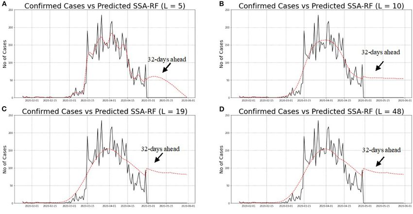
Shaharudin et al.                                                                                        Short-Term Forecasting of COVID-19 Cases

2020. Since then, the Crisis Preparedness Response Centre                  be considered on several factors such as intertwined human,
(CPRC) of Malaysia’s Ministry of Health (MOH) has begun                    social, and political factors. Due to that, predictive monitoring
recording and reporting the cases. The COVID-19 statistics is              paradigm was proposed, which synthesized the prediction and
updated based on the total active cases, recoveries, and casualties        monitoring of the daily COVID-19 cases in the study area.
attained daily from the MOH website.                                       Another forecasting method to predict COVID-19 cases is based
    The worst scenario of SARS-CoV-2 infection to individuals              on machine learning approaches (14–17). Jianxi (13) stated
is fatality. Nevertheless, information on the mechanism of the             that the hybridization model of machine learning approaches
spread of the virus or how it affects a patient seems to be in             produces better performances in predicting cumulative COVID-
scarcity. The Centres for Disease Control and Prevention (CDC)             19 cases with high daily incidence. In addition, the climatic
has verified the COVID-19 human-to-human transmission on                   variables were employed as inputs for proposed forecasting
30th January 2020. As noted by the CDC, COVID-19 can spread                machine learning models.
via droplet, close contact with infected patients, and contact with            Most of the previous studies focuses on the forecasting of
surfaces or objects that has the particles of the virus. It has been       future cases COVID-19. However, the analysis of this pandemic
stipulated that 2–14 days or longer as the incubation period of            pattern is equally important. The proposed method suggested
COVID-19 with 5 days on average (4).                                       by Yogesh (18) considered the trend of new cases of COVID-
    As the impact of this virus is severe, therefore it is important       19 in developing forecasting model. Nevertheless, this model
to be able to detect the pattern and forecast the spread of                didn’t ensure that the trend and noise components in the
confirmed cases is very crucial. For an instance, Zhao et al.              data were clearly separated before the forecasting values were
(5) had proposed a mathematical model to approximate the                   generated. The suitable analytical tools to assess the global
actual COVID-19 cases, including those unreported, for the first           change pattern with uncertainty metrics seem to be rather limited
half of January 2020. It was deduced that the unreported cases             and seldom applied systematically, as it is often presented as
count was 469 between 1st and 15th January 2020. Next, the                 an operational pattern worldwide. Systematically tracking and
estimation of cases from 17th January 2020 onwards revealed that           observing the infectious disease in a specific population and
the case numbers astonishingly encountered a 21-fold upsurge.              presented chronologically at high temporal resolution can lead
This epidemic was predicted to reach its peak in late February             to a modern and sophisticated methodology to perform in-depth
and subside by late April based on the SEIR model combined                 data analysis. Hence, suitable analytical methods for time series
with a machine-learning artificial intelligence (AI) method (6).           data may be used if cases of health outcomes are assembled and
Subsequently, Tang et al. (7) prescribed a mathematical model              aggregated with time units (e.g., weekly or daily basis).
that could estimate the risk of COVID-19 transmission. Based on                Singular Spectrum Analysis (SSA) is a superb and effective
this, the potential number of the basic reproduction was 6.47. It          alternative to address trend components, substantially minimize
also forecasted the total of 7 day confirmed cases with 23rd−29th          noise, and unravel the temporal structure of data minus
January 2020 time interval. Consequently, the estimated peak was           preliminary manipulation (19). Generally, SSA represents
after 2 weeks from the initial date of 23rd January 2020.                  univariate time series transformed into eigenvectors and
    In order to estimate the prolonged COVID-19 human-                     eigenvalues of any trajectory matrix. The SSA refers to a
to-human transmission, data obtained from 47 patients were                 multidimensional analog of principal component analysis
analyzed and resulted in a transmission rate of 0.4 (8). If                (PCA), which is transformed into time series. One function
the duration between the symptom detection and the patient                 of the SSA is to separate the time series data into noise,
hospitalization was halved from the tested study data, the                 trend, and seasonal categories by decomposing the time
transmission rate could reduce to 0.012. In another study,                 series eigen, and later, reconstructing them into group
an estimation of SIR model was exhibited for the COVID-19                  selection (20).
outbreak in Malaysia to predict the short-term daily COVID-                    The SSA, essentially, transforms a single dimension time
19 cases (9). The study reported a transmission rate of 0.22               series into trajectories with multiple dimensions via PCA
by considering that an infected individual can spread the virus            [Singular Value Decomposition (SVD)], as well as reconstruction
to another individual within 4 days. This human-to-human                   (approximation) of chosen Principal Components. However, the
transmission rate of 4 days should be highly considered, or even           separation of the components in this approach depends on
viewed as conservative.                                                    the parameters, which is the selection of window length, L, to
    Furthermore, various researchers have employed Box-Jenkins             form trajectory matrix and identifying the number of leading
time series analysis model in predicting future cases of COVID-            eigentriples (ET), based on eigenvector plot (21). This separation
19 (10–12). For an instance, Rauf and Hannah (12) found out                is crucial in this model to ensure that the trend, seasonal, and
ARIMA (2, 2, 2) model produced the most accurate results                   noise components are easily separated.
compare to others for cases in India. Meanwhile, Jibrin et al.                 Although SSA lacks parametric description and highly relies
(11) recommended that the Autoregressive Fractional Integral               on the length of time series, these flexible SSA models can
Moving Average (ARFIMA) model should be used for further                   recreate the asymmetric shapes of a trend, hence allowing better
analysis of daily COVID-19 new cases. Rauf and Hannah (12)                 prediction of seasonal peaks than can harmonic models. This
found an upward trend of the spread of COVID-19 in Nigeria                 model, when compared to others, is easy to use, dismisses
based on ARIMA (1,1,0) model and more. According to Jianxi                 specification of models of time series and trend, enables
(13), the developed predictive model of COVID-19 cases must                extraction of trend in the presence of noise and oscillations,

Frontiers in Public Health | www.frontiersin.org                       2                                      June 2021 | Volume 9 | Article 604093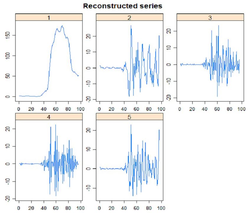
Shaharudin et al.                                                                                                 Short-Term Forecasting of COVID-19 Cases

and involves only two parameters to determine the accuracy and                     cases that resulted in the 2nd wave of COVID-19 pandemic
flexibility in predicting outcomes (22).                                           in Malaysia. With this substantial number, the Malaysian
    As the SSA models are seldom used to assess epidemiological                    Government had announced a Movement Control Order (MCO)
data, this study is set to introduce the SSA model based on                        that took place from 18th to 31st March 2020. The MCO was later
combining forecasting elements of time series analysis known as                    extended to the 4th phase.
Recurrent Forecasting-Singular Spectrum Analysis (RF-SSA). To                         Figure 2 portrays the observed number of cases for COVID-
ensure that this developed model produces significant forecasting                  19 for the last 96 days in Malaysia. The MOH had categorized
results, the selection of the parameter for this model, which are                  four zones of COVID-19 areas in Malaysia based on the areal
the window length, L and the amount of leading eigentriples used,                  cases number. According to the National Security Council
ET, was identified using several tests. The SSA was used in this                   (MKN), the four zones are: (i) green zone for areas with no
study as a base approach to build the forecasting model. The next                  positive case, (ii) yellow zone for areas with one to 20 positive
sections describe the data in detail, followed by several sections                 cases, (iii) orange zone for areas with 21 to 40 positive cases, and
that present the methodology, the results and discussion, and                      (iv) red zone for areas with more than 40 positive cases (23).
finally, the conclusion.                                                              The projection and estimate daily cases of COVID-19
                                                                                   obtained were impacted by the definition of the case reported
                                                                                   to CPRC daily, whereby a large number of pending result test
DATA                                                                               daily was definitely influential to a non-consistent increase in
                                                                                   the number of confirmed cases. The increased prediction cases
Daily COVID-19 prevalence data from 25th January to
                                                                                   are supported by several of the biggest clusters identified by the
29th April 2020 were gathered from MOH records. As this
                                                                                   MOH, such as Seri Petaling Tabligh Cluster, Wedding Kenduri
COVID-19 is a newly-founded virus; no COVID-19 data
                                                                                   in Bandar Baru Bangi, Seri Petaling Sub-Cluster in Rembau, Italy
was available from the previous year. The suspected COVID-
                                                                                   Cluster in Kuching, and Church Fellowship Cluster in Sarawak.
19 cases were diagnosed by using the Reverse Transcription
                                                                                   The new confirmed cases were extremely spiking as the target
Polymerase Chain Reaction (RT-PCR) technique and were
                                                                                   of biology samples were taken directly from highly susceptible
confirmed as COVID-19 case-counts. All fully anonymized,
                                                                                   infected population.
laboratory-confirmed cases were abstracted on COVID-19, in
which 5,945 cases represented COVID-19 infections in all
13 states and 3 federal territories in Malaysia, as recorded                       MATERIALS AND METHODS
by MOH.
   Figure 1 illustrates the total positive cases for COVID-19.                     This section elaborates on the specifics of SSA model and
The figure displays a significant spike in the number of positive                  its components.

 FIGURE 1 | COVID-19 daily confirmed cases in Malaysia from 25th January to 29th April 2020.

Frontiers in Public Health | www.frontiersin.org                               3                                       June 2021 | Volume 9 | Article 604093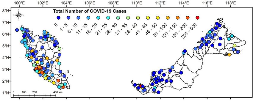
Shaharudin et al. Short-Term Forecasting of COVID-19 Cases
FIGURE 2 | State classification based on number of COVID-19 cases in Malaysia from 25th January to 29th April 2020.
Singular Spectrum Analysis (SSA) Model the eigen time series based on their singular values using
The SSA is a model-free approach that can be applied to all types SVD. The following represents the SVD of the trajectory
of data, regardless of Gaussian or non-Gaussian, linear or non- matrix, Xi where λ1 , . . . , λL are denoted as the eigenvalues
linear, and stationary or non-stationary (24). The daily COVID- of XX T where singular values are arranged in a descending
19 data can be decomposed into several additive components order such that ( σ 1 ≥ σ2 ≥ · · · ≥ σL ) and by
via SSA, which could be defined in the forms of trend, seasonal, U1 , . . . , UL the corresponding eigenvectors. The SVD of X
and noise components (25). The possible application areas can be represented as X = X1 + · · · + XL , where Xi =
√ T
of SSA are diverse (26–28). The SSA is composed of two λi Ui ViT and Vi = X√λUi if (λi = 0 we set Xi = 0).
complementary stages, known as the stages of decomposition and √ i
The set of is called the i − th eigentriple (ET)
λi , Ui , Vi √
reconstruction (29).
of the matrix Xi , and λi are the singular values of the
Stage 1: Decomposition matrix Xi .
The two steps in the decomposition stage are embedding and
SVD. This stage decomposes the series to obtain eigen time
series data. Stage 2: Reconstruction
Step I: Embedding. The first step in basic SSA algorithm is Grouping and diagonal averaging are the two steps in the
embedding, which refers to constructing the original time reconstruction phase. Here, the original series are reconstructed
series into a sequence of lagged vector of size window length, for further analysis, including forecasting.
L by forming lagged vectors, K = T − L + 1 of size L. Step 1: Grouping. Here, the trajectory matrix is divided
Xi = (xi , . . . , xi+L−1 )T (1 ≤ i ≤ K ). into dual groups—trend, seasonal and noise components.
The trajectory matrix of the series X is
Upon setting I = i1 , . . . , ip be a group indices, i1 , . . . , ip
where p < L . Then the matrix XI corresponding to the
x1 x2 x3 · · · xK
group I is defined XI = Xi1 + . . . + Xip . The indices
x2 x3 x4 · · · xK+1
set {1, . . . , L} is divided into m disjoint subsets; I1 , . . . , Im ,
L,K 3
x x 4 x 5 . . . xK+2
X= (X1 ,. . .,XK ) = xij i,j=1 = . .. .. ..
based on the division of elementary matrices into groups of
.. ..
. . . .
m. The retrieved matrices are calculated for I = I1 , . . . , Im
xL xL+1 xL+2 · · · xT which called is eigentriple grouping corresponding to the
representation of X = XI1 + . . . + XIm .
(1) Step 2: Diagonal averaging. The last step in SSA refers to the
transformation of each matrix in the grouped decomposition
The rows and columns of X are subseries of the original one- into new series of length, T.
dimensional time series data and lagged vectors Xi are the • Let Z be L × K matrix with zij , 1 ≤ i ≤ Lelements, 1 ≤ j ≤ K.
columns of the trajectory matrix X. Set L∗ = min (L, K) , K ∗ = max (L, K) , and N = L + K − 1.
Step II: Singular Value Decomposition (SVD). In the second Let zij ∗ = zij if L < K and zij ∗ = zji otherwise. With diagonal
step, the trajectory matrix in Step I is decomposed to obtain averaging, matrix Z is transferred into z1 , . . . , zT based on the
Frontiers in Public Health | www.frontiersin.org 4 June 2021 | Volume 9 | Article 604093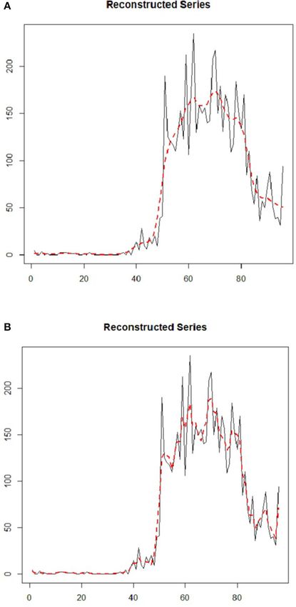
Shaharudin et al. Short-Term Forecasting of COVID-19 Cases
following formula: the signal component in SSA. Therefore, in this study, several
L namely T2 , T5 , 10
T T
, 20 , were investigated on COVID-19 data
1 Pk
∗ 1 ≤ k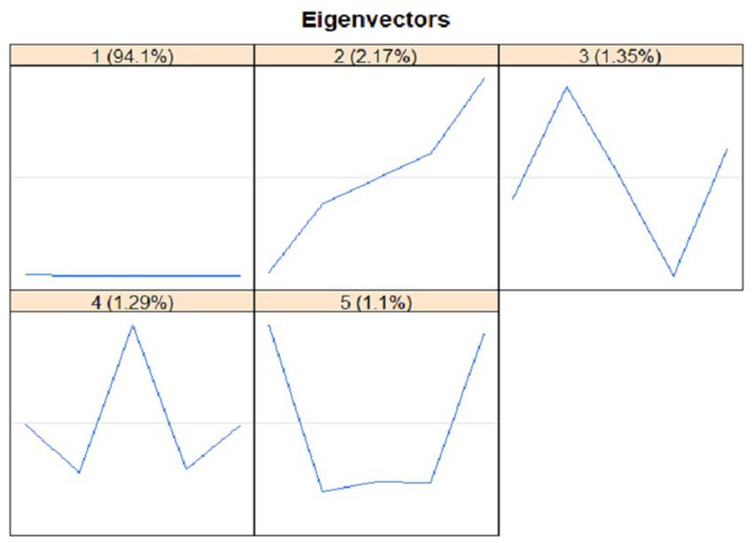
Shaharudin et al.                                                                                    Short-Term Forecasting of COVID-19 Cases

forecasting models. The measurements used in this study are             based on a range from +1 to −1. A value of r that close
Mean Absolute Error (MAE), Mean Forecast Error (MFE), and               to +1 or −1 indicated that the two observed variables are
Root Mean Square Error (RMSE), whereby, the best model is               related to each other. Concurrently, a value of 0 indicates that
selected based on the smallest values for that measurements.            there is no association between two observed variables. The
Meanwhile, the Pearson Correlation Coefficient (r) value is             equations for each of the evaluation performances are shown

 FIGURE 3 | Flow chart of developed forecasting, model of RF-SSA.

Frontiers in Public Health | www.frontiersin.org                    6                                     June 2021 | Volume 9 | Article 604093

Shaharudin et al.                                                                                                      Short-Term Forecasting of COVID-19 Cases

as follows:
                                            n
                                        "                   #
                                            X
                                   −1
                     MAE = n                      yt − ŷ                 (8)
                                         i=1
                                        " n                  #
                                         X
                                   −1

                     MFE = n                      yt − ŷ                 (9)
                                            i=1
                                        "   n
                                                                 #−0.5
                                   −2
                                            X               2
                    RMSE = n                      yt − ŷ                (10)
                                            i=1

                 n( ni=1 xt yt ) −
                   P                Pn          Pn
                                        i=1 xt       i=1 yt
   r = rh
            Pn         Pn         2 i h Pn                 Pn      2 i
                   2                                   2                             FIGURE 4 | Effect of w-correlation based on SSA using COVID-19 data at
          n  i=1 xt −       i=1 xt       n      i=1 yt −       i=1 yt
                                                                                     varied window lengths.
                                                                         (11)

                                                                                    TABLE 1 | Comparison of Singular Spectrum Analysis Prediction Performance for
where yt is the actual values at time t; yt is the predicted values at              Several Window Length (L).
time t; n is the number of observations. Flow chart of developed
forecasting model based on SSA as shown in Figure 3.                                Window Length, L                                                       RMSE

                                                                                    T/2 = 48                                                               29.51
RESULTS AND DISCUSSION                                                              T/5 = 19                                                               29.67

Decomposition and Reconstruction                                                    T/10 = 10                                                              23.97
                                                                                    T/20 = 5                                                               19.12
In the initial stage of this study, COVID-19 data were
decomposed into components by using the SSA model, which
required identification of (L, ET) parameter pair. Here, L denotes
the compromise between statistical confidence and information.
The suitable L value should resolve the varied oscillations                         each square represents the w-correlation strength between two
embedded in the original signal.                                                    components. Meanwhile, Figures 5A–C portrays the tendency
    The performance of the SSA results was determined by                            of the components to form correlation with other components
assessing the w-correlation at distinct window length, L. The w-                    despite signifying weak correlation. Subsequently, this denotes
correlation calculated the separability among noise, trend, and                     that the components of trends are still, to some extent, mixed
seasonal (components of reconstructed time series). Here, L =                       with the noise and seasonal components in SSA and it was
                          T
T/2, T/5, T/10, and 20      , which represent L = 48, 19, 10, and                   rectified by the small window length, L = 5, which is evidently
5, respectively, for T based on 96 daily cases on COVID-19 data                     demonstrated in Figure 5D for better separability.
had been selected. The scales were selected to fit the data of the                      Table 1 presents the reconstructed time series components
time series, apart from striking a balance to achieve a proper lag                  varied window length. The lowest RMSE was observed from
                                                                                          T
vector sequence.                                                                    L = 20  , which had the smallest value amongst other L, indicating
    In Figure 4, the w-correlation is presented based on SSA using                  its suitability based on short-time series of the outbreak data.
daily cases of COVID-19 data at varying window lengths. The                         Meanwhile, the high RMSE values were reported in this study due
w-correlation displayed a declining trend when the total window                     to the high model variance for small sample set.
length declined for SSA approach. The correlations among trend                          The plot of five main eigenvectors is displayed in Figure 6.
and other components should be close to zero for extraction of                      Such plot is beneficial to choose an appropriate group for
trend. This means; the distinct window lengths have an impact on                    the components of time series data, especially to separate
the component’s separability. Besides, the SSA was directed to the                  the components of noise, trend, and seasonal. The retrieved
lowest w-correlation at L = T/20; signifying the best separability                  information may be further analyzed in the step of grouping in
among the reconstructed components as it was the closest to zero.                   RF-SSA. The component of trend was identified from eigenvector
    The graphs in Figures 5A–D illustrate the heat-plot of                          plot, in which seasonal and trend components have sine waves
different window lengths, L, based on w-correlations using                          indicated by the slow cycles found in the graph (high frequency).
the SSA approach. The heat-plot of w-correlation for the                            Meanwhile, the component of noise was represented by the
reconstructed components based on white-black scale ranges                          saw-tooth found in the graph (low frequency). The leading
between 0 and 1 (37). Huge correlation values among the                             eigenvector has nearly continual coordinates, thus corresponding
reconstructed components exhibited the possibility of the                           to a pure smoothing by Bartlett filter (38, 39). The reconstruction
components to form a group while corresponding to the                               result by each of the five ET is presented in Figure 7. The two
same component. As illustrated in Figure 5, the shade of                            figures verified the compatibility of the first and second ET with

Frontiers in Public Health | www.frontiersin.org                                7                                            June 2021 | Volume 9 | Article 604093
Shaharudin et al. Short-Term Forecasting of COVID-19 Cases FIGURE 5 | (A–D) w-correlation plot using SSA with varied windows length (A) L = 48 (B) L = 19 (C) L = 10 (D) L = 5. the trend, whereas the remaining ET had the noise component, of the cases trend and pattern, as it was randomly-tabulated thus irrelevant to trend. as per daily cases (see Figure 8). In Figures 8A, 7, the trend Figure 8 demonstrates the components of the reconstructed was precisely generated by a leading ET, which coincided with time series plot from the trend extracted via RF-SSA for daily the initial reconstructed component exhibited in Figure 8. The COVID-19 cases in Malaysia. The reconstructed series is the trend in Figure 8B was precisely generated by both leading new dataset derived from the original data, which is clear from ET, which coincided with the first and second reconstructed noise. It is a crucial aspect in SSA to ensure that the forecasting components shown in Figure 8. The dashed and straight lines on results are precise and accurate (40). The component of trend the plot denote the reconstructed series based on the extracted in the time series data was used to observe the occurrence trend component from SSA and the COVID-19 original time Frontiers in Public Health | www.frontiersin.org 8 June 2021 | Volume 9 | Article 604093
Shaharudin et al.                                                                                   Short-Term Forecasting of COVID-19 Cases

 FIGURE 6 | Eigenvectors Plot using Singular Spectrum Analysis.

series data, respectively. The plot of reconstructed time series       model are known as SSA-RF. Table 2 presents the summary
components, produced by both leading ET, abides by the original        statistics from the experiment analysis of SSA-RF at several
COVID-19 data although noise component was omitted for L =             windows length.
5 for daily COVID-19 cases in Malaysia.                                   Looking at Table 2, it is apparent that the best performances
   For proper identification of seasonal series components,            can be obtained from L = 5 that has the lowest MAE
the graph of eigenvalues and scatterplots of eigenvectors              of 11.2549 with the highest r of 0.9619, indicating superb
were applied. In order to determine the seasonal series                correlation between confirmed and predicted cases. Moreover,
components using eigenvalues plot, several steps were                  the MFE shows that the SSA-RF algorithm with L = 5,
produced by approximately equal eigenvalues. Figure 9                  tends to under-forecast daily COVID-19 cases by 0.1920%.
portrays the plot of the logarithms of the five singular values        Meanwhile, the second-best model is observed from SSA-
for the COVID-19 cases in Malaysia. It clearly showed                  RF with L = 10 where RMSE is 23.9652, MAE of 14.8890,
that no step produced by approximately equal eigenvalues               r of 0.9402 with MFE of 0.0067%. Meanwhile, L = 19
that corresponded to a sine wave. The scatterplot of                   and L = 48 has the worst performances among all
eigenvectors displays the regular polygons yielded by a pair           models whereby MAE and r for both models are 19.3706
of eigenvectors to demonstrate that the series components              and 0.9086, respectively. Furthermore, MFE statistical results
have produced seasonality components. Based on Figure 10,              showed that both models are over-forecast by 2.82%. Visual
no pair of eigenvectors produced regular polygons. This                inspection on these models performances are presented in
confirmed that the COVID-19 data in Malaysia were not                  Figures 11A–D.
influenced by the seasonality since both figures did not have             Based on Figures 11A–D, it is a clear indication that SSA-RF
sine wave.                                                             models able to capture general pattern of non-linear increasing
                                                                       trend of daily confirmed cases of COVID-19 in Malaysia.
Forecasting Daily COVID-19 Cases Using                                 Detailed analysis from Figure 11A found out that model with
SSA-RF                                                                 L = 5 performed better that other models whereby the model
As mentioned in the previous section, the daily COVID-19               able to follow the actual pattern of daily confirmed cases of
cases in Malaysia were first decomposed and reconstructed              COVID-19. Meanwhile, as can be seen from Figures 11B–D,
using SSA model. The next step in this study is to                     other models which are L = 10, L = 19, and L = 48 unable
predict the future cases of COVID-19 in Malaysia. In this              to follow the actual pattern of the observed data. This is a
stage, an SSA forecasting algorithm known as Recurrent                 clear indication that the models performed poorly as compared
Forecasting were used accordingly. From hereafter, the                 to L = 5 model.

Frontiers in Public Health | www.frontiersin.org                   9                                     June 2021 | Volume 9 | Article 604093
Shaharudin et al. Short-Term Forecasting of COVID-19 Cases FIGURE 7 | First stage: Elementary Reconstructed Series (L = 5). Next, the SSA-RF models were used to predict future cases During the MCO, Malaysians were advised to stay at home starting from 30th April to 31st May 2020. At the time of this as much as possible to minimize the spread of further COVID-19 study, the historical cases from 25th January to 29th April 2020 infections. All schools and most workplaces were closed, and they were used and the future 32 days ahead of COVID-19 cases were directed to work from home except for essential services. had been predicted accordingly. Figures 11A–D illustrates the Traveling ban, restriction movement order including interstate confirmed cases from 25th January to 29th April 2020 and the movement, restriction on gatherings, and public transport forecasted daily cases until 31st May 2020. It is worth noting closure were imposed strictly by the government. Active case that the figures display a noticeable but faint decreasing pattern detection was continued, followed by isolation of the cases, and from 5th April 2020 onwards. One of the contributing factors the close contacts were tested and quarantined to further curb for the decreasing trend was due to the MCO announced by the spread of COVID-19. All these actions successfully plateaued the Malaysian Government which took place on 18th March and reduced the number of COVID-19 cases (Figures 11A–D). 2020. The above figures also illustrate the predicted values of In addition, the cases were reduced due to the incubation period 32 day ahead using SSA-RF algorithm against confirmed cases of the virus between 2 to 14 days, and the recent findings from of COVID-19 in Malaysia. Despite the encouraging statistical WHO has stated that after 5–10 days of the infection, the infected finding based from the historical data and lower under-forecast individual starts to gradually produce neutralizing antibodies value; the SSA-RF models failed to capture the sudden drop which will decrease the risk of transmission to others (41, 42). in the COVID-19 cases, which is considered to have never WHO has also reported three research that found the inability happened before. This sudden drop was highly likely due to of SARS-CoV-2 virus to be cultured after 7–9 days of onset the MCO that was extended to phase-4, which ended on 12th of symptoms (43, 44). From all the latest findings, WHO has May 2020. concluded that after 14 days, the patients are not likely to be Frontiers in Public Health | www.frontiersin.org 10 June 2021 | Volume 9 | Article 604093
Shaharudin et al.                                                                                                  Short-Term Forecasting of COVID-19 Cases

                                                                                FIGURE 9 | Logarithms of five eigenvalues.

 FIGURE 8 | (A,B) Daily COVID-19 cases of reconstructed components from
 extracted trends using SSA at (A) L = 5, ET 1 (B) L = 5, ET 2.

infectious (45). The government’s decision to extend the MCO
up to 12th May had successfully plateaued and reduced the curve                 FIGURE 10 | Plots of eigenvectors (EV) pairs: 1-EV and 2-EV, 2-EV and 3-EV,
as it provides sufficient time to break the virus transmission.                 3-EV and 4-EV, as well as 4-EV and 5-EV for COVID-19 cases.
    Furthermore, the figures showed that different window length
suggested a different forecasted value of future cases. For an
instance, SSA-RF with L = 48. Nineteen and 10 predicted that
there will be insignificant changes in the number of future cases,             June 2020. However, the model unable to predict the date for
while SSA-RF with L = 5 showed there will be a significant drop                total eradication of COVID-19 cases. This is consistent with
in the future cases. Other than that, the model also suggested                 WHO which indicated that this virus will not be eradicated even
that Malaysia will reach single digit in COVID-19 cases by early               after the vaccine is found. It might persist to be endemic in

Frontiers in Public Health | www.frontiersin.org                          11                                            June 2021 | Volume 9 | Article 604093
Shaharudin et al. Short-Term Forecasting of COVID-19 Cases
certain countries and will need cooperation on a global scale and • Recurrent forecasting approach is a better contender than
leveraging tools such as contact tracing and disease surveillance vector approach for forecasting both short and medium
to defeat COVID-19. time series data of SSA. However, under such scenarios,
it is advisable that users also evaluate the performance
of forecasting SSA approach on their data to arrive at a
Limitation of SSA-RF Model complete picture.
Some limitations of this study, which should be emphasized • Although SSA able to capture the pattern of the Coronavirus
when using the SSA-RF model in assessing the pandemic data in COVID-19 cases, however, its ability in predicting the cases
Malaysia, are as follows: accurately is still need to be investigated further.
• The SSA-RF model works best when the data exhibit a stable • Different observed behavior of a dataset might influence the
or consistent pattern over time with a minimum amount of selection of window length.
outlier. This can help to obtain accurate and precise results for • This model did not take into account the effect of incubation
future predictive cases. period in transmission of the virus, the effect of the
• The sudden spike in data leads to low performance of government measures to curb the spread of COVID-19.
forecasting results using this predictive SSA-RF model.
• The SSA-RF model is mainly used to project future values
CONCLUSION
using historical time series data for short-term forecast.
This study assessed the applicability of SSA-RF model in
predicting the COVID-19 cases in Malaysia. The application of
this model is specifically advantageous for the health authorities
TABLE 2 | SSA-RF Prediction Performance Several Window Length (L). in terms of flattening the curve by devising prompt and
effective strategies. This model allows the health authorities to
L MAE r MSE
comprehend the outbreak pattern better. The pattern retrieved
T/2 = 48 19.3706 0.9086 −2.8249 Over-
from the SSA-RF model can be applied to forecast the outbreak
forecast cases growth pattern in Malaysia. The parameters used in this
T/5 = 19 19.3706 0.9086 −2.8249 Over- model were window length, L, and the total of ET employed
forecast for reconstruction, r. The results revealed that parameter L = 5
T/10 = 10 14.8890 0.9402 0.0067 Under- (T/20 ) was suitable for short time series outbreak data and
forecast the appropriate number of leading ET s to obtain was crucial
T/20 = 5 11.2549 0.9619 0.1920 Under- as it affected the forecasting outcomes. Overall, the results
forecast showed that the SSA-RF model could forecast this pandemic
FIGURE 11 | (A–D) Predicted SSA-RF and confirmed cases of COVID-19 in Malaysia for Various Windows Length (L).
Frontiers in Public Health | www.frontiersin.org 12 June 2021 | Volume 9 | Article 604093Shaharudin et al. Short-Term Forecasting of COVID-19 Cases
with reasonable accuracy as the model had under-forecasted by AUTHOR CONTRIBUTIONS
0.1920% with high correlation values between confirmed and
predicted cases. Nevertheless, the SSA-RF model failed to capture SS and SI conceived the presented idea, developed
the sudden drop in COVID-19 cases, likely due to the MCO that the theory, and performed the computations. NH,
was extended to 12th May 2020. In order to improve the accuracy MT, and NS verified the analytical methods and
of the model, more information is required to better predict supervised the findings of this work. All authors
the COVID-19 cases for a long period. In the meantime, case discussed the results and contributed to the
definition and data collection must be maintained in real-time final manuscript.
to enhance the RF-SSA for further evaluation. It is suggested that
the SSA-RF model is enhanced to enable the model to capture FUNDING
sudden and rapid changes in the dataset.
The authors would like to thank the Ministry of Higher
DATA AVAILABILITY STATEMENT Education Malaysia (MOHE) for supporting this research under
Fundamental Research Grant Scheme Vot No. 2019-0132-103-
The raw data supporting the conclusions of this article will be 02 (FRGS/1/2019/STG06/UPSI/02/4) and partially sponsored by
made available by the authors, without undue reservation. Vot No. FRGS/1/2018/STG06/UTHM/03/3.
REFERENCES 15. Rauf HT, Lali MIU, Khan MA, Kadry S, Alolaiyan H, Razaq A, et al.
Time series forecasting of COVID-19 transmission in Asia Pacific countries
1. Chen Y, Liu Q, Guo D. Emerging coronaviruses: genome using deep neural networks. Pers Ubiquitous Comput. (2021) 10:1–
structure, replication, and pathogenesis. J Med Virol. (2020) 18. doi: 10.1007/s00779-020-01494-0
92:2249. doi: 10.1002/jmv.26234 16. Muhammad Attique K, Seifedine K, Yu-Dong Z, Tallha A, Muhammad S,
2. Ge XY, Li JL, Yang XL, Chmura AA, Zhu G, Epstein JH, et al. Isolation and Amjad R, et al. Prediction of COVID-19- pneumonia based on selected deep
characterization of a bat SARS-like coronavirus that uses the ACE2 receptor. features and one class kernel extreme learning machine. Comp Electr Eng.
Nature. (2013) 503:535–8. doi: 10.1038/nature12711 (2021) 90:1–18. doi: 10.1016/j.compeleceng.2020.106960
3. Coronavirus Website - Ministry of Health (2020). Available online at: http:// 17. Matheus Henrique Dal Molin R, Roman Gomes da S, Viviana Cocco
www.moh.gov.my/index.php (accessed April 3, 2020). M, Leandro dos Santos C. Short-term forecasting COVID-19 cumulative
4. Lauer SA, Grantz KH, Bi Q, Jones FK, Zheng Q, Meredith HR, et al. The confirmed cases: perspectives for Brazil. Chaos Solitons Fractals. (2020) 135:1–
incubation period of coronavirus disease 2019 (COVID-19) from publicly 10. doi: 10.1016/j.chaos.2020.109853
reported confirmed cases: estimation and application. Ann Intern Med. (2020) 18. Yogesh G. Transfer learning for COVID-19 cases and deaths using LSTM
172:577–82. doi: 10.7326/M20-0504 network. ISA Transac. (2020). doi: 10.1016/j.isatra.2020.12.057
5. Zhao S, Musa SS, Lin Q, Ran J, Yang G, Wang W, et al. Estimating the 19. Golyandina N Zhigljavsky A. Basic SSA. In: Singular Spectrum Analysis for
Unreported Number of Novel Coronavirus (2019-nCoV) Cases in China in Time Series. Berlin; Heidelberg: Springer (2013). pp. 11–70.
the First Half of January 2020: a data-driven modelling analysis of the early 20. Shaharudin SM, Ahmad N, Zainuddin NH. Modified singular spectrum
outbreak. J Clin Med. (2020) 9:388. doi: 10.3390/jcm9020388 analysis in identifying rainfall trend over Peninsular Malaysia. Indonesian J
6. Yang Z, Zeng Z, Wang K, Wong SS, Liang W, Zanin M, et al. Modified SEIR Electr Eng Comp Sci. (2019) 15:283. doi: 10.11591/ijeecs.v15.i1.pp283-293
and AI prediction of the epidemics trend of COVID-19 in China under public 21. Shaharudin SM, Ahmad N, Yusof F. Effect of window length with singular
health interventions. J Thorac Dis. (2020) 12:165. doi: 10.21037/jtd.2020.02.64 spectrum analysis in extracting the trend signal of rainfall data. Aip Proc.
7. Tang B, Wang X, Li Q, Bragazzi NL, Tang S, Xiao Y, et al. estimation of (2015) 1643:321. doi: 10.1063/1.4907462
the transmission risk of the 2019-nCoV and its implication for public health 22. Fuad MFM, Shaharudin SM, Ismail S, Samsudin NAM, Zulfikri MF.
interventions. J Clin Med. (2020) 9:462. doi: 10.3390/jcm9020462 Comparison of singular spectrum analysis forecasting algorithms for student’s
8. Thompson RN. Novel coronavirus outbreak in Wuhan, China, 2020: intense academic performance during COVID-19 outbreak. IJATEE. (2021) 8:178–89.
surveillance is vital for preventing sustained transmission in new locations. J doi: 10.19101/IJATEE.2020.S1762138
Clin Med. (2020) 9:498. doi: 10.3390/jcm9020498 23. Coronavirus Website - Ministry of Health (2020). Available online at: https://
9. Ariffin MRK, et al. Malaysian COVID-19 Outbreak Data Analysis and kpkesihatan.com/ (accessed April 3, 2020).
Prediction. Institute for Mathematical Research (2020). Available online 24. Deng C. Time Series Decomposition using Singular Spectrum Analysis. Master,
at: http://einspem.upm.edu.my/covid19maths/file/Report_001%20v13.pdf East Tennessee State University (2014).
10. Yemane AG, Daniel A. Trend analysis and forecasting the spread of COVID- 25. Biabanaki M, Eslamian SS, Koupai JA, Canon J, Boni G, Gheysari M.
19 pandemic in ethiopia using box-jenkins modeling procedure. Int J Gen A principal components/singular spectrum analysis approach to enso and
Med. (2021) 2021:1485–98. doi: 10.2147/IJGM.S306250 pdo influences on rainfall in West of Iran. Hydrol Res. (2014) 45:250–
11. Da HL, Youn SK, Young YK, Kwang YS, In HC. Forecasting COVID-19 62. doi: 10.2166/nh.2013.166
confirmed cases usng empirical data analysis in korea. Healthcare (Basel). 26. Rodriguez-Aragon LJ Zhiglkavsky A. Singular spectrum analysis for image
(2021) 9:254. doi: 10.3390/healthcare9030254 processiong. Stat Interface. (2010) 3:419–26. doi: 10.4310/SII.2010.v3.n3.a14
12. Das RC. Forecasting incidences of COVID-19 using Box-Jenkins method for 27. Chau KW, Wu CL. A hybrid model coupled with singular spectrum
the period July 12-Septembert 11, 2020: A study on highly affected countries. analysis for daily rainfall prediction. J Hydroinformat. (2010) 12:458–
Chaos Solitons Fractals. (2020) 140:1–14. doi: 10.1016/j.chaos.2020.110248 73. doi: 10.2166/hydro.2010.032
13. Jianxi L. Forecasting COVID-19 pandemic: unknown unknowns 28. Alexandrov T, Golyandina N, Spirov A. Singular spectrum analysis of
and predictive monitoring. Technol Forecast Soc Change. (2021) gene expression profiles of early drosophila embryo: exponential-in-distance
166:1–4. doi: 10.1016/j.techfore.2021.120602 patterns. Res Lett Signal Proc. (2008) 2008:825758. doi: 10.1155/2008/
14. Ramon Gomes da S, Matheus Henrique Dal Molin R, Viviana Cocco M, 825758
Leandro dos Santos C. Forecasting Brazillian and American COVID-19 cases 29. Carvalho MD Rua A. Real-Time Nowcasting the US Output GAP: Singular
based on artificial intelligence coupled with climatic exogenous variables. Spectrum Analysis at Work. Lisboa: Banco De Portugal (2014) ISBN 978-989-
Chaos Solitons Fractals. (2020) 139:1–13. doi: 10.1016/j.chaos.2020.110027 678-304-4.
Frontiers in Public Health | www.frontiersin.org 13 June 2021 | Volume 9 | Article 604093Shaharudin et al. Short-Term Forecasting of COVID-19 Cases
30. Danilov D. Principal components in time series forecast. J Comput Graph Stat. 40. Hassani H, Zhigljavsky A. Singular spectrum analysis: methodology
(1997) 6:112–21. doi: 10.1080/10618600.1997.10474730 and application to economics data. J Syst Sci Complex. (2009)
31. Danilov D. The Caterpillar method for time series forecasting. In: Danilov 22:372. doi: 10.1007/s11424-009-9171-9
D, Zhigljavsky A, editors. Principal Components of Time Series: The 41. Wolfel R, Corman VM, Guggemos W, Seilmaier M, Zange S, Müller MA,
Caterpillar Method. St. Petersburg: University of St. Petersburg (1997). et al. Virological assessment of hospitalized patients with COVID-19. Nature.
p. 73–104. (2020) 581:465–9. doi: 10.1038/s41586-020-2196-x
32. Golyandina N, Nekrutkin V, Zhigljavsky A. Analysis of Time Series Structure: 42. Atkinson B, Petersen E. SARS-CoV-2 shedding and infectivity. Lancet. (2020)
SSA and Related Techniques. New York, NY: Chapman & Hall/CRC (2001). 395:1339–40. doi: 10.1016/S0140-6736(20)30868-0
33. Shaharudin SM, Ismail S, Samsudin MS, Azid A, Tan ML, Basri MAA. 43. Bullard J, Dusk K, Funk D, Strong JE, Alexander D, Garnett L, et al. Predicting
Prediction of epidemic trends in COVID-19 with mann-kendall and recurrent infectious SARS-CoV-2 from diagnostic samples. Clin Infect Dis. (2020)
forecasting-singular spectrum analysis. Sains Malays. (2021) 50:1131–42. 71:2663–6. doi: 10.1093/cid/ciaa638
doi: 10.17576/jsm-2021-5004-23 44. Peng Z, Xing-Lou Y, Xian-Guang W, Ben H, Lei Z, Wei Z, et al. A pneumonia
34. Alonso FJ, Salgado DR, Cuadrado J, Pintado P. Automatic smoothing of outbreak associated with a new coronavirus of probable bat origin. Nature.
raw kinematics signals using SSA andcluster analysis. In: Euromech Solid (2020) 579:270–3. doi: 10.1038/s41586-020-2012-7
Mechanics Conference. Lisbon (2009). p. 1–9. 45. Centers for Disease Control and Prevention, Coronavirus Disease 2019
35. Golyandina N, Shlemov A. Variations of singular spectrum analysis (COVID-19). Symptom-Based Strategy to Discontinue Isolation for Persons
for separability improvement: non-orthogonal decompositions of With COVID-19. (2020). Available online at: https://www.who.int/news-
time series. Stat Interface. (2014) 8:277–94. doi: 10.4310/SII.2015. room/commentaries/detail/criteria-for-releasing-COVID-19-patients-
v8.n3.a3 from-isolation (accessed June 12, 2020).
36. Golyandina NE, Korobeynikov A. Basic singular spectrum
analysis forecasting with R. Comput Stat Data Anal. (2014) Conflict of Interest: The authors declare that the research was conducted in the
71:934–54. doi: 10.1016/j.csda.2013.04.009 absence of any commercial or financial relationships that could be construed as a
37. Hassani H. Singular spectrum analysis: methodology and comparison. J Data potential conflict of interest.
Sci. (2007) 5:239–57. Available online at: https://mpra.ub.uni-muenchen.de/
4991/ Copyright © 2021 Shaharudin, Ismail, Hassan, Tan and Sulaiman. This is an open-
38. Golyandina N, Nekrutkin V, Zhigljavsky A. Analysis of Time Series access article distributed under the terms of the Creative Commons Attribution
Structure: SSA and Related Techniques. New York, NY; London: Chapman License (CC BY). The use, distribution or reproduction in other forums is permitted,
Hall/CRC (2001). provided the original author(s) and the copyright owner(s) are credited and that the
39. Mahmoudvand R, Konstantinides D, Rodrigues PC. Forecasting Mortality original publication in this journal is cited, in accordance with accepted academic
Rate by Multivariate Singular Spectrum Analysis. John Wiley & Sons, Ltd. practice. No use, distribution or reproduction is permitted which does not comply
(2017) 33:717–32. doi: 10.1002/asmb.2274 with these terms.
Frontiers in Public Health | www.frontiersin.org 14 June 2021 | Volume 9 | Article 604093You can also read