Shyft v4.8: a framework for uncertainty assessment and distributed hydrologic modeling for operational hydrology - GMD
←
→
Page content transcription
If your browser does not render page correctly, please read the page content below
Geosci. Model Dev., 14, 821–842, 2021
https://doi.org/10.5194/gmd-14-821-2021
© Author(s) 2021. This work is distributed under
the Creative Commons Attribution 4.0 License.

Shyft v4.8: a framework for uncertainty assessment and distributed
hydrologic modeling for operational hydrology
John F. Burkhart1 , Felix N. Matt1,2 , Sigbjørn Helset2 , Yisak Sultan Abdella2 , Ola Skavhaug3 , and Olga Silantyeva1
1 Department of Geosciences, University of Oslo, Oslo, Norway
2 Statkraft
          AS, Lysaker, Norway
3 Expert Analytics AS, Oslo, Norway

Correspondence: John F. Burkhart (john.burkhart@geo.uio.no)

Received: 12 February 2020 – Discussion started: 4 May 2020
Revised: 14 October 2020 – Accepted: 16 October 2020 – Published: 5 February 2021

Abstract. This paper presents Shyft, a novel hydrologic           1   Introduction
modeling software for streamflow forecasting targeted for
use in hydropower production environments and research.
The software enables rapid development and implementa-            Operational hydrologic modeling is fundamental to several
tion in operational settings and the capability to perform dis-   critical domains within our society. For the purposes of flood
tributed hydrologic modeling with multiple model and forc-        prediction and water resource planning, the societal benefits
ing configurations. Multiple models may be built up through       are clear. Many nations have hydrological services that pro-
the creation of hydrologic algorithms from a library of well-     vide water-related data and information in a routine manner.
known routines or through the creation of new routines, each      The World Meteorological Organization gives an overview
defined for processes such as evapotranspiration, snow accu-      of the responsibilities of these services and the products they
mulation and melt, and soil water response. Key to the de-        provide to society, including monitoring of hydrologic pro-
sign of Shyft is an application programming interface (API)       cesses, provision of data, water-related information includ-
that provides access to all components of the framework           ing seasonal trends and forecasts, and, importantly, decision
(including the individual hydrologic routines) via Python,        support services (World Meteorological Organization, 2006).
while maintaining high computational performance as the              Despite the abundantly clear importance of such opera-
algorithms are implemented in modern C++. The API al-             tional systems, implementation of robust systems that are
lows for rapid exploration of different model configurations      able to fully incorporate recent advances in remote sensing,
and selection of an optimal forecast model. Several differ-       distributed data acquisition technologies, high-resolution
ent methods may be aggregated and composed, allowing di-          weather model inputs, and ensembles of forecasts remains
rect intercomparison of models and algorithms. In order to        a challenge. Pagano et al. (2014) provide an extensive review
provide enterprise-level software, strong focus is given to       of these challenges, as well as the potential benefits afforded
computational efficiency, code quality, documentation, and        by overcoming some relatively simple barriers. The Hydro-
test coverage. Shyft is released open-source under the GNU        logic Ensemble Prediction EXperiment (https://hepex.irstea.
Lesser General Public License v3.0 and available at https:        fr/, last access: 22 November 2020) is an activity that has
//gitlab.com/shyft-os (last access: 22 November 2020), facil-     been ongoing since 2004, and there is extensive research on
itating effective cooperation between core developers, indus-     the importance of the role of ensemble forecasting to reduce
try, and research institutions.                                   uncertainty in operational environments (e.g., Pappenberger
                                                                  et al., 2016; Wu et al., 2020).
                                                                     As most operational hydrological services are within the
                                                                  public service, government policies and guidelines influence
                                                                  the area of focus. Recent trends show efforts towards increas-
                                                                  ing commitment to sustainable water resource management,

Published by Copernicus Publications on behalf of the European Geosciences Union.
822                                                                                            J. F. Burkhart et al.: Shyft v4.8

disaster avoidance and mitigation, and the need for integrated     ple of the scale of the challenge is well-defined in Zappa
water resource management as climatic and societal changes         et al. (2008) in which the authors’ contributions to the re-
are stressing resources.                                           sults of the Demonstration of Probabilistic Hydrological and
    For hydropower production planning, operational hydro-         Atmospheric Simulation of flood Events in the Alpine re-
logic modeling provides the foundation for energy market           gion (D-PHASE) project under the Mesoscale Alpine Pro-
forecasting and reservoir management, addressing the inter-        gramme (MAP) of the WMO World Weather Research Pro-
ests of both power plant operators and governmental reg-           gram (WWRP) are highlighted. In particular, they had the
ulations. Hydropower production accounts for 16 % of the           goal to operationally implement and demonstrate a new gen-
world’s electricity generation and is the leading renewable        eration of flood warning systems in which each catchment
source for electricity (non-hydro-renewable and waste sum          had one or more hydrological models implemented. How-
up to about 7 %). Between 2007 and 2015, the global hy-            ever, following the “demonstration” period, “no MAP D-
dropower capacity increased by more than 30 % (World En-           PHASE contributor was obviously able to implement its hy-
ergy Council, 2016). In many regions around the globe, hy-         drological model in all basins and couple it with all avail-
dropower is therefore playing a dominant role in the regional      able deterministic and ensemble numerical weather predic-
energy supply. In addition, as energy production from renew-       tion (NWP) models”. This presumably resulted from the
able sources with limited managing possibilities (e.g., from       complexity of the configurations required to run multiple
wind and solar) grows rapidly, hydropower production sites         models with differing domain configurations, input file for-
equipped with pump storage systems provide the possibility         mats, operating system requirements, and so forth.
to store energy efficiently at times when total energy produc-        There is an awareness in the hydrologic community re-
tion surpasses demands. Increasingly critical to the growth        garding the nearly profligate abundance of hydrologic mod-
of energy demand is the proper accounting of water use and         els. Recent efforts have proposed the development of a
information to enable water resource planning (Grubert and         community-based hydrologic model (Weiler and Beven,
Sanders, 2018).                                                    2015). The WRF-Hydro platform (Gochis et al., 2018) is a
    Great advances in hydrologic modeling are being made           first possible step in that direction, along with the Structure
in several facets: new observations are becoming available         for Unifying Multiple Modelling Alternatives (SUMMA)
through novel sensors (McCabe et al., 2017), numerical             (Clark et al., 2015a), a highly configurable and flexible plat-
weather prediction (NWP) and reanalysis data are increas-          form for the exploration of structural model uncertainty.
ingly reliable (Berg et al., 2018), detailed estimates of quan-    However, the WRF-Hydro platform is computationally ex-
titative precipitation estimates (QPEs) are available as model     cessive for many operational requirements, and SUMMA
inputs (Moreno et al., 2012, 2014; Vivoni et al., 2007; Ger-       was designed with different objectives in mind than what
mann et al., 2009; Liechti et al., 2013), there are improved al-   has been developed within Shyft. For various reasons (see
gorithms and parameterizations of physical processes (Kirch-       Sect. 1.2) the development of Shyft was initiated to fill a gap
ner, 2006), and, perhaps most significantly, we have greatly       in operational hydrologic modeling.
advanced in our understanding of uncertainty and the quan-            Shyft is a modern cross-platform open-source toolbox that
tification of uncertainty within hydrologic models (West-          provides a computation framework for spatially distributed
erberg and McMillan, 2015; Teweldebrhan et al., 2018b).            hydrologic models suitable for inflow forecasting for hy-
Anghileri et al. (2016) evaluated the forecast value of long-      dropower production. The software is developed by Statkraft
term inflow forecasts for reservoir operations using ensemble      AS, Norway’s largest hydropower company and Europe’s
streamflow prediction (ESP) (Day, 1985). Their results show        largest generator of renewable energy, in cooperation with
that the value of a forecast using ESP varies significantly as a   the research community. The overall goal for the toolbox
function of the seasonality, hydrologic conditions, and reser-     is to provide Python-enabled high-performance components
voir operation protocols. Regardless, having a robust ESP          with industrial quality and use in operational environments.
system in place allows operational decisions that will create      Purpose-built for production planning in a hydropower envi-
value. In a follow-on study, Anghileri et al. (2019) showed        ronment, Shyft provides tools and libraries that also aim for
that preprocessing of meteorological input variables can also      domains other than hydrologic modeling, including model-
significantly benefit the forecast process.                        ing energy markets and high-performance time series calcu-
    A significant challenge remains, however, in environments      lations, which will not be discussed herein.
that have operational requirements. In such an environment,           In order to target hydrologic modeling, the software allows
24/7 up-time operations, security issues, and requirements         the creation of model stacks from a library of well-known hy-
from information technology departments often challenge            drologic routines. Each of the individual routines are devel-
introducing new or “innovative” approaches to modeling.            oped within Shyft as a module and are defined for processes
Furthermore, there is generally a requirement to maintain          such as evapotranspiration, snow accumulation and melt, and
an existing model configuration while exploring new possi-         soil water response. Shyft is highly extensible, allowing oth-
bilities. Often, the implementation of two parallel systems        ers to contribute or develop their own routines. Other mod-
is daunting and presents a technical roadblock. An exam-           ules can be included in the model stack for improved han-

Geosci. Model Dev., 14, 821–842, 2021                                                https://doi.org/10.5194/gmd-14-821-2021
J. F. Burkhart et al.: Shyft v4.8                                                                                             823

dling of snowmelt or to preprocess and interpolate point in-       of uncertainty, evaluated satellite data forcing, and explored
put time series of temperature and precipitation (for example)     data assimilation routines for snow.
to the geographic region. Several different methods may be
easily aggregated and composed, allowing direct intercom-          1.1   Other frameworks
parison of algorithms. The method stacks operate on a one-
dimensional geo-located “cell”, or a collection of cells may       To date, a large number of hydrological models exist, each
be constructed to create catchments and regions within a do-       differing in the input data requirements, level of details in
main of interest. Calibration of the methods can be conducted      process representation, flexibility in the computational sub-
at the cell, catchment, or region level.                           unit structure, and availability of code and licensing. In the
   The objectives of Shyft are to (i) provide a flexible hy-       following we provide a brief summary of several models that
drologic forecasting toolbox built for operational environ-        have garnered attention and a user community but were ul-
ments, (ii) enable computationally efficient calculations of       timately found not optimal for the purposes of operational
hydrologic response at the regional scale, (iii) allow for using   hydrologic forecasting at Statkraft.
the multiple working hypothesis to quantify forecast uncer-           Originally aiming for incorporation in general circula-
tainties, (iv) provide the ability to conduct hydrologic sim-      tion models, the Variable Infiltration Capacity (VIC) model
ulations with multiple forcing configurations, and (v) fos-        (Liang et al., 1994; Hamman et al., 2018) has been used
ter rapid implementation into operational modeling improve-        to address topics ranging from water resources management
ments identified through research activities.                      to land–atmosphere interactions and climate change. In the
   To address the first and second objectives, computa-            course of its development history of over 20 years, VIC has
tional efficiency and well-test-covered software have been         served as both a hydrologic model and land surface scheme.
paramount. Shyft is inspired by research software developed        The VIC model is characterized by a grid-based representa-
for testing the multiple working hypothesis (Clark et al.,         tion of the model domain, statistical representation of sub-
2011). However, the developers felt that more modern cod-          grid vegetation heterogeneity, and multiple soil layers with
ing standards and paradigms could provide significant im-          variable infiltration and nonlinear base flow. Inclusion of to-
provements in computational efficiency and flexibility. Using      pography allows for orographic precipitation and tempera-
the latest C++ standards, a templated code concept was cho-        ture lapse rates. Adaptations of VIC allow the representation
sen in order to provide flexible software for use in business-     of water management effects and reservoir operation (Hadde-
critical applications. As Shyft is based on advanced tem-          land et al., 2006a, b, 2007). Routing effects are typically ac-
plated C++ concepts, the code is highly efficient and able to      counted for within a separate model during post-processing.
take advantage of modern-day compiler functionality, min-             Directed towards use in cold and seasonally snow-covered
imizing risk of faulty code and memory leaks. To address           small- to medium-sized basins, the Cold Regions Hydro-
the latter two objectives, the templated language functional-      logical Model (CRHM) is a flexible object-oriented soft-
ity allows for the development of different algorithms that are    ware system. CRHM provides a framework that allows the
then easily implemented into the framework. An application         integration of physically based parameterizations of hydro-
programming interface (API) is provided for accessing and          logical processes. Current implementations consider cold-
assembling different components of the framework, includ-          region-specific processes such as blowing snow, snow in-
ing the individual hydrologic routines. The API is exposed         terception in forest canopies, sublimation, snowmelt, infil-
to both the C++ and Python languages, allowing for rapid           tration into frozen soils, and hillslope water movement over
exploration of different model configurations and selection        permafrost (Pomeroy et al., 2007). CRHM supports both spa-
of an optimal forecast model. Multiple use cases are enabled       tially distributed and aggregated model approaches. Due to
through the API. For instance, one may choose to explore the       the object-oriented structure, CRHM is used as both a re-
parameter sensitivity of an individual routine directly, or one    search and predictive tool that allows rapid incorporation of
may be interested purely in optimized hydrologic prediction,       new process algorithms. New and already existing imple-
in which case one of the predefined and optimized model            mentations can be linked together to form a complete hy-
stacks, a sequence of routines forming a hydrologic model,         drological model. Model results can either be exported to a
would be of interest.                                              text file, ESRI ArcGIS, or a Microsoft Excel spreadsheet.
   The goal of this paper is two-fold: to introduce Shyft and         The Structure for Unifying Multiple Modelling Alterna-
to demonstrate some recent applications that have used het-        tives (SUMMA) (Clark et al., 2015a, b) is a hydrologic
erogeneous data to configure and evaluate the fidelity of sim-     modeling approach that is characterized by a common set
ulation. First, we present the core philosophical design deci-     of conservation equations and a common numerical solver.
sions in Sect. 2 and provide and overview of the architecture      SUMMA constitutes a framework that allows users to test,
in Sect. 3. The model formulation and hydrologic routines          apply, and compare a wide range of algorithmic alternatives
are discussed in Sects. 4 and 5. Secondly, we provide a re-        for certain aspects of the hydrological cycle. Models can
view of several recent applications that have addressed issues     be applied to a range of spatial configurations (e.g., nested
                                                                   multi-scale grids and hydrologic response units). By enabling

https://doi.org/10.5194/gmd-14-821-2021                                                Geosci. Model Dev., 14, 821–842, 2021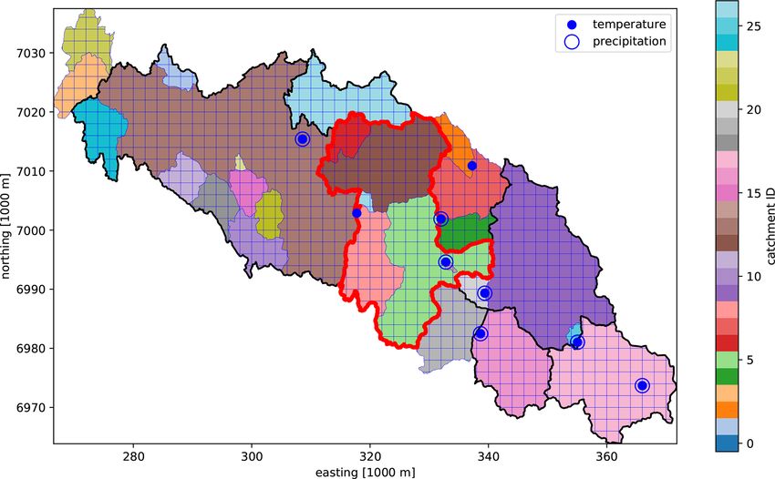
824                                                                                           J. F. Burkhart et al.: Shyft v4.8

model intercomparison in a controlled setting, SUMMA is             Notable complications arise in continuously operating en-
designed to explore the strengths and weaknesses of certain      vironments. Current IT practices in the industry impose se-
model approaches and provides a basis for future model de-       vere constraints upon any changes in the production systems
velopment.                                                       in order to ensure required availability and integrity. This
   While all these models provide functionality similar to       challenges the introduction of new modeling approaches, as
(and beyond) Shyft’s model structure, such as flexibility in     service level and security are forcedly prioritized above in-
the computational subunit structure, allowing for using the      novation. To keep the pace of research, the operational re-
multiple working hypothesis, and statistical representation      quirements are embedded into automated testing of Shyft.
of sub-grid land type representation, the philosophy behind      Comprehensive unit test coverage provides proof for all lev-
Shyft is fundamentally different from the existing model         els of the implementation, whilst system and integration tests
frameworks. These differences form the basis of the decision     give objective means to validate the expected service behav-
to develop a new framework, as outlined in the following sec-    ior as a whole, including validation of known security con-
tion.                                                            siderations. Continuous integration aligned with agile (iter-
                                                                 ative) development cycle minimize human effort for the ap-
1.2   Why build a new hydrologic framework?                      propriate quality level. Thus, adoption of the modern prac-
                                                                 tices balances tough IT demands with motivation for rapid
Given the abundance of hydrologic models and modeling            progress. Furthermore, C++ was chosen as a programming
systems, the question must be asked as to why there is a         language for the core functionality. In spite of a steeper learn-
need to develop a new framework. Shyft is a distributed mod-     ing curve, templated code provides long-term advantages for
eling environment intended to provide operational forecasts      reflecting the target architecture in a sustainable way, and the
for hydropower production. We include the capability of the      detailed documentation gives a comprehensive explanation
exploration of multiple hydrologic model configurations, but     of the possible entry points for the new routines.
the framework is somewhat more restricted and limited from          One of the key objectives was to create a well-defined API,
other tools addressing the multiple model working hypoth-        allowing for an interactive configuration and development
esis. As discussed in Sect. 1.1, several such software solu-     from the command line. In order to provide the flexibility
tions exist; however, for different reasons these were found     needed to address the variety of problems met in operational
not suitable for deployment. The key criteria we sought when     hydrologic forecasting, flexible design of workflows is criti-
evaluating other software included the following:                cal. By providing a Python/C++ API, we provide access to
  – open-source license and clear license description;           Shyft functionality via the interpreted high-level program-
                                                                 ming language Python. This concept allows a Shyft user to
  – readily accessible software (e.g., not trial- or
                                                                 design workflows by writing Python scripts rather than re-
    registration-based);
                                                                 quiring user input via a graphical user interface (GUI). The
  – high-quality code that is                                    latter is standard in many software products targeted toward
                                                                 hydropower forecasting but was not desired. Shyft develop-
       – well-commented,
                                                                 ment is conducted by writing code in either Python or C++
       – has modern standards,                                   and is readily scripted and configurable for conducting sim-
       – is API-based and not a graphical user interface         ulations programmatically.
         (GUI), and
       – is highly configurable using object-oriented stan-
                                                                 2   Design principles
         dards;
  – well-documented software.                                    Shyft is a toolbox that has been purpose-developed for op-
                                                                 erational, regional-scale hydropower inflow forecasting. It
   As we started the development of Shyft, we were unable
                                                                 was inspired from previous implementations of the multi-
to find a suitable alternative based on the existing packages
                                                                 ple working hypothesis approach to provide the opportunity
at the time. In some cases the software is simply not read-
                                                                 to explore multiple model realizations and gain insight into
ily available or suitably licensed. In others, documentation
                                                                 forecast uncertainty (Kolberg and Bruland, 2014; Clark et al.,
and test coverage were not sufficient. Most prior implementa-
                                                                 2015b). However, key design decisions have been taken to-
tions of the multiple working hypothesis have a focus on the
                                                                 ward the requirement to provide a tool suitable for opera-
exploration of model uncertainty or provide more complex-
                                                                 tional environments which vary from what may be priori-
ity than required, therefore adding data requirements. While
                                                                 tized in a pure research environment. In order to obtain the
Shyft provides some mechanisms for such investigation, we
                                                                 level of code quality and efficiency required for use in the hy-
have further extended the paradigm to enable efficient eval-
                                                                 dropower market, we adhered to the following design princi-
uation of multiple forcing datasets in addition to model con-
                                                                 ples.
figurations, as this is found to drive a significant component
of the variability.

Geosci. Model Dev., 14, 821–842, 2021                                              https://doi.org/10.5194/gmd-14-821-2021
J. F. Burkhart et al.: Shyft v4.8 825
2.1 Enterprise-level software 2.5 Hot service
Large organizations often have strict requirements regarding Perhaps the most ambitious principle is to develop a tool that
software security, testing, and code quality. Shyft follows the may be implemented as a hot service. The concept is that
latest code standards and provides well-documented source rather than model results being saved to a database for later
code. It is released as open-source software and maintained at analysis and visualization, a practitioner may request simu-
https://gitlab.com/shyft-os (last access: 22 November 2020). lation results for a certain region at a given time by running
All changes to the source code are tracked, and changes are the model on the fly without writing results to file. Further-
run through a test suite, greatly reducing the risk of errors more, perhaps one would like to explore slight adjustments
in the code. This process is standard operation for software to some model parameters, requiring recomputation, in real
development but remains less common for research software. time. This vision will only be actualized through the devel-
Test coverage is maintained at greater than 90 % of the whole opment of extremely fast and computationally efficient algo-
C++ code base. Python coverage is about 60 % overall, in- rithms.
cluding user interface, which is difficult to test. The hydrol- The adherence to a set of design principles creates
ogy part has Python test coverage of more than 70 % on av- a software framework that is consistently developed and
erage and is constantly validated via research activities. easily integrated into environments requiring tested, well-
commented, well-documented, and secure code.
2.2 Direct connection to data stores
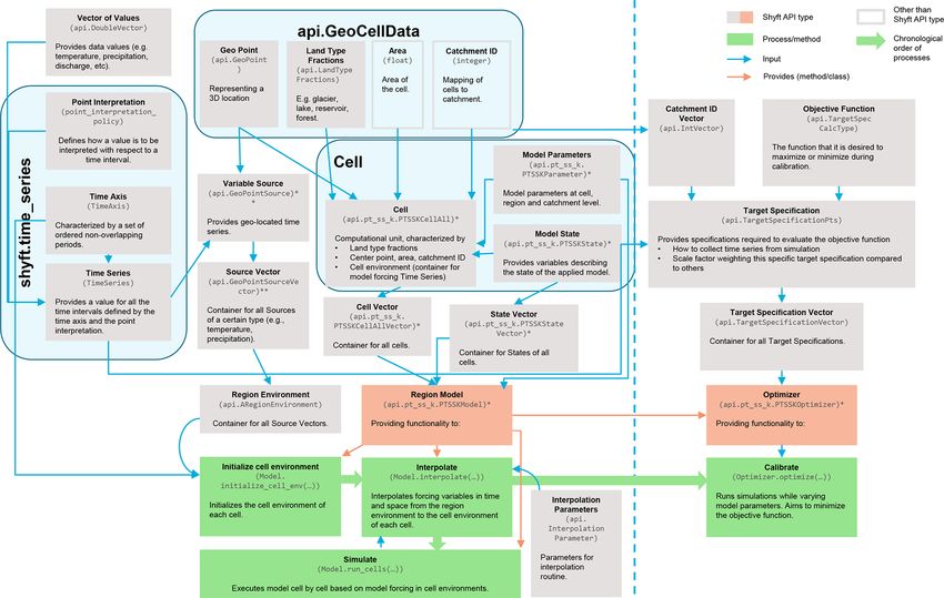
A central philosophy of Shyft is that “data should live at 3 Architecture and structure
the source!”. In operational environments, a natural chal-
lenge exists between providing a forecast as rapidly as pos- Shyft is distributed in three separate code repositories and a
sible and conducting sufficient quality assurance and control “docker” repository as described in Sect. 7.
(QA/QC). As the QA/QC process is often ongoing, there may Shyft utilizes two different code bases (see overview given
be changes to source datasets. For this reason, intermediate in Fig. 1). Basic data structures, hydrologic algorithms, and
data files should be excluded, and Shyft is developed with models are defined in Shyft’s core, which is written in C++
this concept in mind. Users are encouraged to create their in order to provide high computational efficiency. In addi-
own “repositories” that connect directly to their source data, tion, an API exposes the data types defined in the core to
regardless of the format (see Sect. 4). Python. Model instantiation and configuration can therefore
be utilized from pure Python code. In addition, Shyft pro-
2.3 Efficient integration of new knowledge vides functionalities that facilitate the configuration and real-
ization of hydrologic forecasts in operational environments.
Research and development (R&D) are critical for organiza-
These functionalities are provided in Shyft’s orchestration
tions to maintain competitive positions. There are two pre-
and are part of the Python code base. As one of Shyft’s de-
vailing pathways for organizations to conduct R&D: through
sign principles is that data should live at the source rather
internal divisions or through external partnerships. The chal-
than Shyft requiring a certain input data format, data repos-
lenge of either of these approaches is that often the results
itories written in Python provide access to data sources. In
from the research – or “project deliveries” – are difficult to
order to provide robust software, automatic unit tests cover
implement efficiently in an existing framework. Shyft pro-
large parts of both code bases. In the following section, de-
vides a robust operational hydrologic modeling environment,
tails to each on the architectural constructs are given.
while providing flexible “entry points” for novel algorithms,
and the ability to test the algorithms in parallel with opera- 3.1 Core
tional runs.
The C++ core contains several separate code folders: core
2.4 Flexible method application
– for handling framework-related functionality, like serial-
Aligning with the principle of enabling rapid implementation ization and multithreading; time series – aimed at operating
of new knowledge, it is critical to develop a framework that with generic time series and hydrology; and all the hydro-
enables flexible, exploratory research. The ability to quantify logic algorithms, including structures and methods to manip-
uncertainty is highly sought. One is able to explore epistemic ulate with spatial information.1 The design and implemen-
uncertainty (Beven, 2006) introduced through the choice of tation of models aim for multicore operations to ensure uti-
hydrologic algorithm. Additionally, mechanisms are in place lization of all computational resources available. At the same
to enable selection of alternative forcing datasets (including 1 The core also contains dtss (time series handling services, en-
point vs. distributed) and to explore variability resulting from ergy_market) algorithms related to energy market modeling and
these data. web_api (web services), which are out of scope of this introductory
paper.
https://doi.org/10.5194/gmd-14-821-2021 Geosci. Model Dev., 14, 821–842, 2021
826                                                                                              J. F. Burkhart et al.: Shyft v4.8

time, design considerations ensure the system may be run on         to NumPy and SciPy documentation.2 Here we will try
multiple nodes. The core algorithms utilize third-party, high-      to give an overview of the types typically used in ad-
performance, multithreaded libraries. These include the stan-       vanced simulations via API (the comprehensive set of exam-
dard C++ (latest version), boost (Demming et al., 2010), ar-        ples is available at https://gitlab.com/shyft-os/shyft-doc/tree/
madillo (Sanderson and Curtin, 2016), and dlib (King, 2009)         master/notebooks/api, last access: 22 November 2020).
libraries, altogether leading to efficient code.                       shyft.time_series provides mathematical and statistical op-
   The Shyft core itself is written using C++ templates from        erations and functionality for time series. A time series can
the abovementioned libraries and also provides templated al-        be an expression or a concrete point time series. All time
gorithms that consume template arguments as input param-            series do have a time axis (TimeAxis – a set of ordered non-
eters. The algorithms also return templates in some cases.          overlapping periods), values (api.DoubleVector), and a point
This allows for high flexibility and simplicity without sacri-      interpretation policy (point_interpretation_policy). The time
ficing performance. In general, templates and static dispatch       series can provide a value for all the intervals, and the point
are used over class hierarchies and inheritance. The goal to-       interpretation policy defines how the values should be inter-
ward faster algorithms is achieved via optimizing the com-          preted: (a) the point instant value is valid at the start of the
position, enabling multithreading, and the ability to scale out     period, linear between points, extends flat from the last point
to multiple nodes.                                                  to +∞, and undefined before the first value; it is typical for
                                                                    state variables, like water level and temperature, measured
                                                                    at 12:00 local time. (b) The point average value represents
3.2   Shyft API
                                                                    an average or constant value over the period; it is typical for
                                                                    model input and results, like precipitation and discharge. The
The Shyft API exposes all relevant Shyft core implemen-             TimeSeries functionality includes the following: resampling
tations that are required to configure and utilize models to        – average, accumulate, time_shift; statistics – min–max, cor-
Python. The API is therefore the central part of the Shyft ar-      relation by Nash–Sutcliffe, Kling–Gupta; filtering – convo-
chitecture that a Shyft user is encouraged to focus on. An          lution, average, derivative; quality and correction – min–max
overview of fundamental Shyft API types and how they can            limits, replace by linear interpolation or replacement time se-
be used to initialize and apply a model is shown in Fig. 2.         ries; partitioning and percentiles.
   A user aiming to simulate hydrological models can do this           api.GeoCellData represents common constant cell proper-
by writing pure Python code without ever being exposed to           ties across several possible models and cell assemblies. The
the C++ code base. Using Python, a user can configure and           idea is that most of our algorithms use one or more of these
run a model and access data at various levels such as model         properties, so we provide a common aspect that keeps this
input variables, model parameters, and model state and out-         together. Currently it keeps the mid-point api.GeoPoint, the
put variables. It is of central importance to mention that as       Area, api.LandTypeFractions (forest, lake, reservoir, glacier,
long as a model instance is initiated, all of these data are kept   and unspecified), Catchment ID, and routing information.
in the random access memory of the computer, which allows              Cell is a container of GeoCellData and TimeSeries of
a user to communicate with a Shyft model and its underlying         model forcings (api.GeoPointSource). The cell is also spe-
data structures using an interactive Python command shell           cific to the Model selected, so api.pt_ss_k.PTSSKCellAll ac-
such as the Interactive Python (IPython; Fig. 3). In this man-      tually represents cells of a Priestley–Taylor–Skaugen–Snow–
ner, a user could, for instance, interactively configure a Shyft    Kirchner (PTSSK) type, related to the stack selected (de-
model, feed forcing data to it, run the model, and extract and      scribed in Sect. 5.2). The structure collects all the necessary
plot result variables. Afterwards, as the model object is still     information, including cell state, cell parameters, and simu-
instantiated in the interactive shell, a user could change the      lation results. Cell Vector (api.pt_ss_k.PTSSKCellAllVector)
model configuration, e.g., by updating certain model param-         is a container for the cells.
eters, rerun the model, and extract the updated model results.         Region Model (api.pt_ss_k.PTSSKModel) contains
Exposing all relevant Shyft core types to an interpreted pro-       all the Cells and also Model Parameters at region and
gramming language provides a considerable level of flexibil-        catchment level (api.pt_ss_k.PTSSKParameter). Ev-
ity at the user level that facilitates the realization of a large   erything is vectorized, so, for example, Model State
number of different operational setups. Furthermore, using          vector in the form of api.pt_ss_k.PTSSKStateVector col-
Python offers a Shyft user access to a programming language         lects together the states of each model cell. The region
with intuitive and easy-to-learn syntax, wide support through       model is a provider of all functionality available: ini-
a large and growing user community, over 300 standard li-           tialization (Model.initialize_cell_env(...)), interpolation
brary modules that contain modules and classes for a wide           (Model.interpolate(...)), simulation (Model.run_cells(...)),
variety of programming tasks, and cross-platform availabil-         and calibration (Optimizer.optimize(...)), wherein the op-
ity.
   All Shyft classes and methods available through the API             2 https://docs.scipy.org/doc/numpy-1.15.0/docs/howto_
follow the documentation standards introduced in the guide          document.html (last access: 22 November 2020)

Geosci. Model Dev., 14, 821–842, 2021                                                 https://doi.org/10.5194/gmd-14-821-2021
J. F. Burkhart et al.: Shyft v4.8 827
Figure 1. Architecture of Shyft.
timizer is api.pt_ss_k.PTSSKOptimizer – also a construct Shyft accesses data required to run simulations through
within the model purposed specifically for the calibration. It repositories (Fowler, 2002). The use of repositories is driven
is in the optimizer, where the Target Specification resides. by the aforementioned design principle to have a “direct con-
To guide the model calibration we have a GoalFunction that nection to the data store”. Each type of repository has a spe-
we try to minimize based on the TargetSpecification. cific responsibility, a well-defined interface, and may have a
The Region Model is separated from Region Environ- multitude of implementations of these interfaces. The data
ment (api.ARegionEnvironment), which is a container for all accessed by repositories usually originate from a relational
Source vectors of certain types, like temperature and precip- database or file formats that are well-known. In practice, data
itation, in the form of api.GeoPointSourceVector. are never accessed in any way other than through these inter-
Details on the main components of Fig. 2 are pro- faces, and the intention is that data are never converted into a
vided in following sections. Via API the user can interact particular format for Shyft. In order to keep code in the Shyft
with the system at any possible step, so the frame- orchestration at a minimum, repositories are obliged to return
work gives flexibility at any stage of simulation, but the Shyft API types. Shyft provides interfaces for the following
implementation resides in the C++ part, keeping the effi- repositories.
ciency at the highest possible levels. The documentation
page at https://gitlab.com/shyft-os/shyft-doc/blob/master/ Region model repository. The responsibility is to pro-
notebooks/shyft-intro-course-master/run_api_model.ipynb vide a configured region model, hiding away any
(last access: 22 November 2020) provides a simple single- implementation-specific details regarding how the
cell example of Shyft simulation via API, which extensively model configuration and data are stored (e.g., in a
explains each step. NetCDF database, a geographical information system).
3.3 Repositories Geo-located time series repository. The responsibility is to
provide all meteorology- and hydrology-relevant types
Data required to conduct simulations are dependent on the of geo-located time series needed to run or calibrate
hydrological model selected. However, at present the avail- the region model (e.g., data from station observations,
able routines require at a minimum temperature and precipi- weather forecasts, climate models).
tation, and most also use wind speed, relative humidity, and
radiation. More details regarding the requirements of these Interpolation parameter repository. The responsibility is to
data are given in Sect. 5. provide parameters for the interpolation method used in
the simulation.
https://doi.org/10.5194/gmd-14-821-2021 Geosci. Model Dev., 14, 821–842, 2021828 J. F. Burkhart et al.: Shyft v4.8
Figure 2. Description of the main Shyft API types and how they are used in order to construct a model. API types used for running
simulations are shown to the left of the dashed line; additional types used for model calibration are to the right of it. ∗ Different API types
exist for different Shyft models dependent on the choice of the model. For this explanatory figure we use a PTSSK stack, which is an
acronym for Priestley–Taylor–Skaugen–Snow–Kirchner. ∗∗ Different API types exist for different types of input variables (e.g., temperature,
precipitation, relative humidity, wind speed, radiation).
State repository. The responsibility is to provide model provides a collection of utilities that allow users to configure,
states for the region model and store model states for run, and post-process simulations. Orchestration provides for
later use. two main objectives.
Shyft provides implementations of the region model repos- The first is to offer an easy entry point for modelers seek-
itory interface and the geo-located time series repository in- ing to use Shyft. By using the orchestration, users require
terface for several datasets available in NetCDF formats. only a minimum of Python scripting experience in order to
These are mostly used for documentation and testing and can configure and run simulations. However, the Shyft orches-
likewise be utilized by a Shyft user. Users aiming for an op- tration gives only limited functionality, and users might find
erational implementation of Shyft are encouraged to write it limiting to their ambitions. For this reason, Shyft users are
their own repositories following the provided interfaces and strongly encouraged to learn how to effectively use Shyft API
examples rather than converting data to the expectations of functionality in order to be able to enjoy the full spectrum of
the provided NetCDF repositories. opportunities that the Shyft framework offers for hydrologic
modeling.
3.4 Orchestration Secondly, and importantly, it is through the orchestration
that full functionality can be utilized in operational environ-
We define “orchestration” as the composition of the simula- ments. However, as different operational environments have
tion configuration. This included defining the model domain, different objectives, it is likely that an operator of an op-
selection of forcing datasets and model algorithms, and pre- erational service wants to extend the current functionalities
sentation of the results. In order to facilitate the realization of the orchestration or design a completely new one from
of simple hydrologic simulation and calibration tasks, Shyft scratch suitable to the needs the operator defines. The orches-
provides an additional layer of Python code. The Shyft or-
chestration layer is built on top of the API functionalities and
Geosci. Model Dev., 14, 821–842, 2021 https://doi.org/10.5194/gmd-14-821-2021J. F. Burkhart et al.: Shyft v4.8 829
Figure 3. Simplified example showing how a Shyft user can configure a Shyft model using the Shyft API (from shyft import api)
and (interactive) Python scripting. In line 2, the model to be used is chosen. In line 3 a model cell suitable to the model is initiated. In line 4 a
cell vector, which acts as a container for all model cells, is initiated and the cell is appended to the vector (line 5). In line 6, a parameter object
is initiated that provides default model parameters for the model domain. Based on the information contained in the cell vector (defining
the model domain), the model parameters, and the model itself, the region model can be initiated (line 7) and, after some intermediate steps
not shown in this example, stepped forward in time (line n). The example is simplified in that it gives a rough overview of how to use
the Shyft API but does not provide a real working example. The functionality shown herein provides a small subset of the functionalities
provided by the Shyft API. For more complete examples we recommend the Shyft documentation (https://shyft.readthedocs.io, last access:
22 November 2020).
tration provided in Shyft then rather serves as an introductory model domain is composed of a user-defined number of cells
example. and catchments and is called a region. A Shyft region thus
specifies the geographical properties required in a hydrologic
simulation.
4 Conceptual model For computations, the cells are vectorized rather than rep-
resented on a grid, as is typical for spatially distributed mod-
The design principles of Shyft led to the development of a els. This aspect of Shyft provides significant flexibility and
framework that attempts to strictly separate the model do- efficiency in computation.
main (region) from the model forcing data (region environ-
ment) and the model algorithms in order to provide a high
degree of flexibility in the choice of each of these three ele- 4.2 Region environment
ments. In this section how a model domain is constructed in
Shyft is described and how it is combined with a set of mete- Model forcing data are organized in a construct called a re-
orological forcing data and a hydrological algorithm in order gion environment. The region environment provides contain-
to generate an object that is central to Shyft, the so-called ers for each variable type required as input to a model. Me-
region model. For corresponding Shyft API types, see Fig. 2. teorological forcing variables currently supported are tem-
perature, precipitation, radiation, relative humidity, and wind
4.1 Region: the model domain speed. Each variable container can be fed a collection of geo-
located time series, referred to as sources, each providing
In Shyft, a model domain is defined by a collection of geo- the time series data for the variables coupled with methods
located subunits called cells. Each cell has certain properties that provide information about the geographical location for
such as land type fractions, area, geographic location, and a which the data are valid. The collections of sources in the
unique identifier specifying to which catchment the cell be- region environment can originate from, e.g., station observa-
longs (the catchment ID). Cells with the same catchment ID tions, gridded observations, gridded numerical weather fore-
are assigned to the same catchment and each catchment is casts, or climate simulations (see Fig. 4). The time series of
defined by a set of catchment IDs (see Fig. 4). The Shyft these sources are usually presented in the original time reso-
https://doi.org/10.5194/gmd-14-821-2021 Geosci. Model Dev., 14, 821–842, 2021830 J. F. Burkhart et al.: Shyft v4.8
Figure 4. A Shyft model domain consisting of a collection of cells. Each cell is mapped to a catchment using a catchment ID. The default cell
shape in this example is square; however, note that at the boundaries cells are not square but instead follow the basin boundary polygon. The
red line indicates a catchment that could be defined by a subset of catchment IDs. The framework would allow for using the full region, but
simulating only within this catchment. The blue circles mark the geographical location of meteorological data sources, which are provided
by the region environment.
lution as available in the database from which they originate. The region model provides the following key functionali-
That is, the region environment typically provides meteoro- ties that allow us to simulate the hydrology of a region.
logical raw data, with no assumption on spatial properties of
the model cells or the model time step used for simulation. – Interpolation of meteorological forcing data from the
source locations to the cells using a user-defined inter-
4.3 Model polation method and interpolation from the source time
resolution to the simulation time resolution. A construct
The model approach used to simulate hydrological processes named cell environment, a property of each cell, acts as
is defined by the user and is independent of the choice of a container for the interpolated time series of forcing
the region and region environment configurations. In Shyft, variables. Available interpolation routines are descried
a model defines a sequence of algorithms, each of which de- in Sect. 5.1.
scribes a method to represent certain processes of the hydro-
logical cycle. Such processes might be evapotranspiration, – Running the model forward in time. Once the interpo-
snow accumulation and melt processes, or soil response. The lation step is performed, the region model is provided
respective algorithms are compiled into model stacks, and with all data required to predict the temporal evolution
different model stacks differ in at least one method. Cur- of hydrologic variables. This step is done through cell-
rently, Shyft provides four different model stacks, described by-cell execution of the model stack. This step is com-
in more detail in Sect. 5.2. putationally highly efficient due to enabled multithread-
ing that allows parallel execution on a multiprocessing
4.4 Region model system by utilizing all central processing units (CPUs)
unless otherwise specified.
Once a user has defined the region representing the model
domain, the region environment providing the meteorolog- – Providing access to all data related to region and model.
ical model forcing, and the model defining the algorithmic All data that are required as input to the model and gen-
representation of hydrologic processes, these three objects erated during a model run are stored in memory and can
can be combined to create a region model, an object that is be accessed through the region model. This applies to
central to Shyft. model forcing data at source and cell level, model pa-
rameters at region and catchment level, static cell data,
Geosci. Model Dev., 14, 821–842, 2021 https://doi.org/10.5194/gmd-14-821-2021J. F. Burkhart et al.: Shyft v4.8 831
and time series of model state result variables. The lat- a model stack cell by cell. This section gives an overview of
ter two are not necessarily stored by default in order to the methods implemented for interpolation and hydrologic
achieve high computational efficiency, but collection of modeling.
those can be enabled prior to a model run.
5.1 Interpolation
A simplified example of how to use the Shyft
API to configure a Shyft region model is shown In order to interpolate model forcing data from the source
in Fig. 3, or one can consult the documentation: locations to the cell locations, Shyft provides two different
https://gitlab.com/shyft-os/shyft-doc/blob/master/ interpolation algorithms: interpolation via inverse distance
notebooks/shyft-intro-course-master/run_api_model.ipynb weighting and Bayesian kriging. However, it is important to
(last access: 22 November 2020). mention that Shyft users are not forced to use the internally
provided interpolation methods. Instead, the provided inter-
4.5 Targets polation step can be skipped and input data can be fed di-
rectly to cells, leaving it up to the Shyft user how to interpo-
Shyft provides functionality to estimate model parameters by late and/or downscale model input data from source locations
providing implementation of several optimization algorithms to the cell domain.
and goal functions. Shyft utilizes optimization algorithms
from dlib (http://www.dlib.net/optimization.html#find_min_ 5.1.1 Inverse distance weighting
bobyqa, last access: 22 November 2020): Bound Optimiza-
tion BY Quadratic Approximation (BOBYQA), which is Inverse distance weighting (IDW) (Shepard, 1968) is the pri-
a derivative-free optimization algorithm and global func- mary method used to distribute model forcing time series to
tion search algorithm explained in Powell (2009) (http:// the cells. The implementation of IDW allows a high degree of
dlib.net/optimization.html#global_function_search, last ac- flexibility in the approach of a choice of models for different
cess: 22 November 2020) that performs global optimization variables.
of a function, subject to bound constraints.
In order to optimize model parameters, model results are 5.1.2 Bayesian temperature kriging
evaluated against one or several target specifications (Gupta
et al., 1998). Most commonly, simulated discharge is evalu- As described in Sect. 5.1.1 we provide functionality to use a
ated with observed discharge; however, Shyft supports fur- height-gradient-based approach to reduce the systematic er-
ther variables such as mean catchment snow water equiv- ror when estimating the local air temperature based on re-
alence (SWE) and snow-covered area (SCA) to estimate gional observations. The gradient value may either be calcu-
model parameters. This enables a refined condition of the lated from the data or set manually by the user.
parameter set for variables for which a more physical model In many cases, this simplistic approach is suitable for the
may be used and high-quality data are available. This ap- purposes of optimizing the calibration. However, if one is
proach is being increasingly employed in snow-dominated interested in greater physical constraints on the simulation,
catchments (e.g., Teweldebrhan et al., 2018a; Riboust et al., we recognize that the gradient is often more complicated and
2019). An arbitrary number of target time series can be eval- varies both seasonally and with local weather. There may be
uated during a calibration run, each representing a different situations in which insufficient observations are available to
part of the region and/or time interval and step. The over- properly calculate the temperature gradient, or potentially the
all evaluation metric is calculated from a weighted average local forcing at the observation stations is actually represen-
of the metric of each target specification. To evaluate perfor- tative of entirely different processes than the one for which
mance users can specify Nash–Sutcliffe (Nash and Sutcliffe, the temperature is being estimated. An alternative approach
1970), Kling–Gupta (Gupta et al., 1998), or absolute differ- has therefore been implemented in Shyft that enables apply-
ence or root mean square error (RMSE) functions. The user ing a method that would buffer the most severe local effects
can specify which model parameters to optimize, giving a in such cases.
search range for each of the parameters. In order to provide The application of Bayes’ theorem is suitable for such
maximum speed, the optimized models are used during cali- weighting of measurement data against prior information.
bration so that the CPU and memory footprints are minimal. Shyft provides a method that estimates a regional height gra-
dient and sea level temperature for the entire region, which
together with elevation data subsequently model a surface
5 Hydrologic modeling temperature.
Modeling the hydrology of a region with Shyft is typi- 5.1.3 Generalization
cally done by first interpolating the model forcing data from
the source locations (e.g., atmospheric model grid points or The IDW in Shyft is generalized and adapted to the practi-
weather stations) to the Shyft cell location and then running calities using available grid forecasts:
https://doi.org/10.5194/gmd-14-821-2021 Geosci. Model Dev., 14, 821–842, 2021832 J. F. Burkhart et al.: Shyft v4.8
1. selecting the neighbors that should participate in the Table 1. Input data requirements per model.
IDW individually for each destination point;
Input variable Unit Model stacks
– The Z scale allows the selection to discriminate
Temperature ◦C all model stacks
neighbors that are of different height (e.g., precipi-
tation, relative humidity, prefer same heights); Precipitation mm h−1 all model stacks
Radiation W m−2 all model stacks
– the number of neighbors that should be chosen for
Wind speed m s−1 PTGSK
any given interpolation point; and Relative humidity % PTGSK
– excluding neighbors with distances larger than a
specified limit.
hydrologic calculations. In these remaining model stacks, the
2. Given the neighbors selected according to (1), a trans-
model stack naming convention provides information about
formation technique or method adapted to the signal
the hydrologic methods used in the respective model.
type is applied to project the signal from its source po-
sition into the destination position. The weight scaling 5.3 PTGSK
factor is 1/pow(distance, distance_scale_factor).
– PT (Priestley–Taylor)
– Temperature has several options available.
Method for evapotranspiration calculations according to
– The temperature lapse rate is computed us- Priestley and Taylor (1972).
ing the nearest neighbors with sufficient and/or
maximized vertical distance. – GS (Gamma-Snow)
– The full 3D temperature flux vector is derived Energy-balance-based snow routine that uses a gamma
from the selected points, and then the vertical function to represent sub-cell snow distribution (Kol-
component is used. berg et al., 2006).
– For precipitation, – K (Kirchner)
(scale_factor)(z distance in meters/100.0) , the scale Hydrologic response routine based on Kirchner (2009).
factor specified in the parameter, and the z distance
as the source–destination distance. In the PTGSK model stack, the model first uses Priestley–
Taylor to calculate the potential evapotranspiration based on
– Radiation: allows for slope and factor adjustment temperature, radiation, and relative humidity data (see Ta-
on the destination cell. ble 1 for an overview of model input data). The calculated
potential evaporation is then used to estimate the actual evap-
5.2 Model stacks
otranspiration using a simple scaling approach. The Gamma-
In Shyft, a hydrologic model is a sequence of hydrologic Snow routine is used to calculate snow accumulation and
methods and a called model stack. Each method of the model melt-adjusted runoff using time series data for precipitation
stack describes a certain hydrologic process, and the model and wind speed in addition to the input data used in the
stack typically provides a complete rainfall–runoff model. Priestley–Taylor method. Glacier melt is accounted for using
In the current state, the model stacks provided in Shyft dif- a simple temperature index approach (Hock, 2003). Based on
fer mostly in the representation of snow accumulation and the snow- and ice-adjusted available liquid water, Kirchner’s
melt processes due to the predominant importance of snow approach is used to calculate the catchment response. The
in the hydropower production environments of Nordic coun- PTGSK model stack is the only model in Shyft which pro-
tries, where the model was operationalized first. These model vides an energy-balance approach to the calculation of snow
stacks provide sufficient performance in the catchments for accumulation and melt processes.
which the model has been evaluated; however, it is expected
5.4 PTSSK
that for some environments with different climatic condi-
tions more advanced hydrologic routines will be required, – SS (Skaugen Snow)
and therefore new model stacks are in active development. Temperature-index-model-based snow routine with a
Furthermore, applying Shyft in renewable energy production focus on snow distribution according to Skaugen and
environments other than hydropower (e.g., wind power) is Randen (2013) and Skaugen and Weltzien (2016).
realizable but will not be discussed herein.
Currently, there are four model stacks available that un- As with the PTGSK model stack, all calculations are iden-
dergo permanent development. With the exception of the tical with the exception that the snow accumulation and melt
HBV (Hydrologiska Byråns Vattenbalansavdeling) (Lind- processes are calculated using the Skaugen Snow routine.
ström et al., 1997) model stack, the distinction for the re- The implementation strictly separates potential melt calcula-
maining three model options is the snow routine used in the tions from snow distribution calculations, making it an easy
Geosci. Model Dev., 14, 821–842, 2021 https://doi.org/10.5194/gmd-14-821-2021You can also read