Simulation of a flash flood event over the Adriatic Sea with a high resolution atmosphere-ocean-wave coupled system - Nature
←
→
Page content transcription
If your browser does not render page correctly, please read the page content below
www.nature.com/scientificreports
OPEN Simulation of a flash‑flood
event over the Adriatic
Sea with a high‑resolution
atmosphere–ocean–wave coupled
system
Antonio Ricchi1,2,3*, Davide Bonaldo3, Guido Cioni6, Sandro Carniel3,5 &
Mario Marcello Miglietta4
On the morning of September 26, 2007, a heavy precipitation event (HPE) affected the Venice lagoon
and the neighbouring coastal zone of the Adriatic Sea, with 6-h accumulated rainfall summing up
to about 360 mm in the area between the Venetian mainland, Padua and Chioggia. The event was
triggered and maintained by the uplift over a convergence line between northeasterly flow from
the Alps and southeasterly winds from the Adriatic Sea. Hindcast modelling experiments, using
standalone atmospheric models, failed to capture the spatial distribution, maximum intensity and
timing of the HPE. Here we analyze the event by means of an atmosphere-wave-ocean coupled
numerical approach. The combined use of convection permitting models with grid spacing of 1 km,
high-resolution sea surface temperature (SST) fields, and the consistent treatment of marine
boundary layer fluxes in all the numerical model components are crucial to provide a realistic
simulation of the event. Inaccurate representations of the SST affect the wind magnitude and,
through this, the intensity, location and time evolution of the convergence zone, thus affecting the
HPE prediction.
Recent studies1,2 have shown that Heavy Precipitation Events (HPEs) in the Mediterranean coastal regions are
in many ways dependent on Sea Surface Temperature (SST). SST magnitude and spatial patterns control the
air-sea energy exchange, thus modifying the environment where precipitating systems develop by modulating
evaporation3, modifying the atmospheric low-level stability4, and also changing the amount of precipitable
water through moistening of the marine boundary layer (MABL). In this way, the air-sea interaction affects the
structure and organization of precipitating systems, their lifecycle, severity, propagation speed and track, thus
impacting the rain intensity1,5,6. Also, they may induce a rapid intensification of deep moist convection, leading
in the Mediterranean to extreme precipitation a mounts7,8, to the transition of baroclinic cyclones into cyclones
with tropical c haracteristics9,10, or to the intensification of mesocyclonic waterspouts which, after moving inland,
may produce devastating c onsequences11.
In search of an accurate representation of HPEs in NWP (Numerical Weather Prediction) models, increas-
ing attention is now being paid to coupled atmosphere–ocean–wave numerical systems, since they treat in a
consistent way the air-sea interface processes relative to heat, mass and momentum exchanges12. However, the
difficulties related to their implementation (need of extensive computational resources) and validation (lack of
data over the sea) still prevent these tools from being routinely employed for operational purposes.
The aim of this study is to explore how the use of a coupled modelling system may influence the simulation of
regional and local scale atmospheric patterns of a HPE over the Mediterranean region and to investigate whether
it may provide more predictive skills than standalone atmospheric models. The event investigated in this study
1
Department of Physical and Chemical Sciences, University of L’Aquila, 67100, Via Vetoio (Coppito 1, Edificio
“Renato Ricamo”), L’Aquila, Italy. 2Center of Excellence in Telesensing of Environment and Model Prediction of
Severe Events (CETEMPS), Via Vetoio (Coppito 1, Edificio “Renato Ricamo”), L’Aquila 67100, Italy. 3CNR-ISP,
Institute of Polar Sciences, via Torino 155, I‑30172, Venezia Mestre, Venice, Italy. 4CNR-ISAC, Padua/Lecce,
Italy. 5STO CMRE, V.le San Bartolomeo 400, I‑19126, La Spezia, Italy. 6Max Planck Institute for Meteorology,
Hamburg, Germany. *email: antonio.ricchi@univaq.it
Scientific Reports | (2021) 11:9388 | https://doi.org/10.1038/s41598-021-88476-1 1
Vol.:(0123456789)
www.nature.com/scientificreports/
took place in the Venice lagoon on September 26, 2007, locally producing more than 360 mm in 12 h13,14. This
event caused severe damages to infrastructures, public services and private property, and was poorly predicted
by both real-time operational models and hindcast simulations. Hereafter, we investigate the relevance of the
effect of small-scale SST features, which are not resolved in the lower boundary conditions generally used to
drive NWP models, for the proper simulation of rainfall amount and localization in this HPE. By doing this, an
outline of the processes controlling these events will emerge, alongside with a discussion on the implications
and requirements in terms of model coupling and parameterization strategies.
“Case study and simulation setup” section describes the case study and the numerical setup of the simula-
tions implemented here. Results are shown in “Results” section, followed by discussion in “Discussion” section.
Conclusions are finally drawn in “Conclusions” section.
Case study and simulation setup
The HPE near Venice of September 26, 2 00715 was generated by a Mesoscale Convective System (MCS). The latter
was triggered and sustained by the convergence between dry and cold air coming from the Alps (barrier wind),
with warmer and humid air from the southern Adriatic (Sirocco wind). These two different air masses met in
proximity of the northeastern Italian coastline, triggering intense convective activity. Deep moist convection
remained active in the same area for about 6 h (from 04 to 10 UTC) and was organized in the V-shape typical
of a back-building convective s ystem16, with an estimated cloud top temperature of about − 55 °C at 12 km
height15. The multicell system remained quasi-stationary, slowly moving towards the s ea14, and caused intense
precipitation in an area of about 10 k m2, with accumulated rainfall of 360 mm in 6 h (Fig. 1) in the small town
of Campagna Lupia, about 180 mm in Mira and 130 mm in Venice. The spatial pattern and the intensity of the
rainfall were retrieved from observational records provided by the Veneto Region Environmental Protection
Agency (ARPAV) rain gauge n etwork15. The three-dimensional features of the system were reconstructed based
on the data from Teolo C-Band radar located in Monte Grande (472 m a.s.l., approximately 40 km south-west
of the event), processed by ARPAV. This event is classified in the category of “Upstream” HPEs15, where low-
level blocking conditions persist, the upstream profile is unstable and the level of free convection is located at
low altitude, thus the uplift over the barrier wind cold layer is strong enough to trigger convection. In order to
simulate the HPE, we employ the COAWST numerical framework (Coupled Ocean Atmosphere Waves Sedi-
ment Transport model17–19), which consists of a coupled system among the atmospheric model WRF20 (Weather
Research and Forecasting system), the oceanic model ROMS21 (Regional Oceanographic Modelling System),
and the wave model S WAN22 (Simulating WAves in Nearshore). WRF is a state-of-the-art numerical weather
prediction system that solves the fully compressible, nonhydrostatic Euler equations. In the present study, the
version ARW-3.8 has been configured in a 3-domain setup with 1:5 nesting ratio, from 25 km down to 1 km grid
spacing (the coarser grid covers the whole central Europe, the inner domain the northern Adriatic Sea). As a first
step, in order to identify the best numerical and physical configuration, several stand-alone sensitivity tests were
carried out. In detail, we have tested the sensitivity to the number of vertical levels (from 45 to 75, in step of 10),
to the soil dataset (USGS and MODIS), and, following the results in1, to different parameterization schemes avail-
able in WRF, relative to microphysics, planetary boundary layer, cumulus convection (in the coarser domains),
and nesting technique (2-way vs 1-way). The most accurate results, in terms of accumulated precipitations and
localization of HPE, were obtained using 55 vertical levels (with the first level at 15 m above the ground), the
MODIS soil dataset (ORNL DAAC. 2018. MODIS and VIIRS Land Products Global Subsetting and Visualization
Tool), initial and boundary conditions provided by the FNL dataset (Final Reanalysis of the Global Forecasting
System), and 2-way nesting technique. The sensitivity to physics showed that better results were obtained using
the Kain-Fritsch cumulus scheme23 only for the two coarser domains, the WSM 5-class microphysics scheme24,
the Mellor-Yamada-Janjic Planetary Boundary Layer scheme25, and RRTMG26 (Rapid Radiative Transfer Model
Radiation Scheme) for longwave and shortwave radiation. ROMS and SWAN use the same 1-km grid covering the
entire Adriatic Sea, with an open boundary at the Otranto Strait. ROMS entails the 3-D hydrostatic formulation of
the Reynolds-averaged Navier–Stokes equations, discretizing the water column into 30 terrain-following vertical
levels, whereas SWAN provides a phase-averaged description of the generation, propagation and dissipation of
the sea state by dividing the spectral domain into 25 logarithmically-spaced frequencies and 36 directions. This
configuration was successfully used in previous works in the Adriatic S ea27,28, to which the reader is referred for
further details. The coupling frequency, which plays a fundamental role in the description of the energy fluxes
at the air-sea interface, was set to 600 s for the reference run, since this value provided better results in terms of
statistical indices compared to a sensitivity test using 3600 s, as shown in Fig. 1.
The COAWST modeling suite has been tested in 2 different groups of configurations (shown in Table 1), all
starting at 00 UTC, September 25 and ending at 00 UTC, September 27. In the first group, COAWST has been
used as a stand-alone atmospheric system (the WRF model). The simulations differ in terms of SST forcing and
are as follows:
1) RTG: initial and boundary conditions are taken from satellite data in the NOAA database (RTG_SST), pro-
vided at 8.3 km resolution every 6 h (Fig. 2a);
2) ROMS: SST fields are extracted from the spin-up simulation2 (a one-way coupled atmosphere–ocean simu-
lation starting at 00 UTC, September 1, with ocean variables initialized by the CMEMS fi elds29) used to
initialize the AOW and AO run. Boundary conditions are provided every 6 h to force WRF as a standalone
model. Thus, compared to the RTG simulation, this run uses a higher-resolution dataset, obtained from a
coupled model simulation; compared to the coupled run, it has the same initial condition but it does not
treat in a consistent way the air-sea fluxes;
Scientific Reports | (2021) 11:9388 | https://doi.org/10.1038/s41598-021-88476-1 2
Vol:.(1234567890)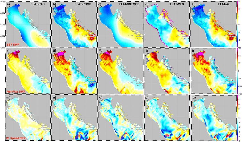
www.nature.com/scientificreports/
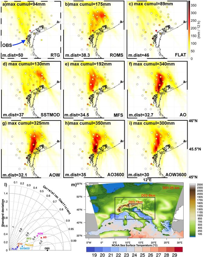
Figure 1. Panels (a–i) 6 h accumulated precipitation observed in each ARPAV station (coloured dots), together
with simulated precipitation (mm) as resulting from the different runs. Plots refer to the period 06–12 UTC,
2007 September, 26: max cumul is the sum of maximum hourly values associated with the storm cell; m.dist is
the average distance (in km) between the storm location and Campagna Lupia (where the most intense rainfall
was observed and highlighted with “OBS” in panel (a); panel l: Taylor diagram of the timeseries of hourly
rainfall maximum associated with the storm cell. Panel m shows the numerical domains, topography and
satellite SST (resolution 8.3 km) at 06 UTC.
Scientific Reports | (2021) 11:9388 | https://doi.org/10.1038/s41598-021-88476-1 3
Vol.:(0123456789)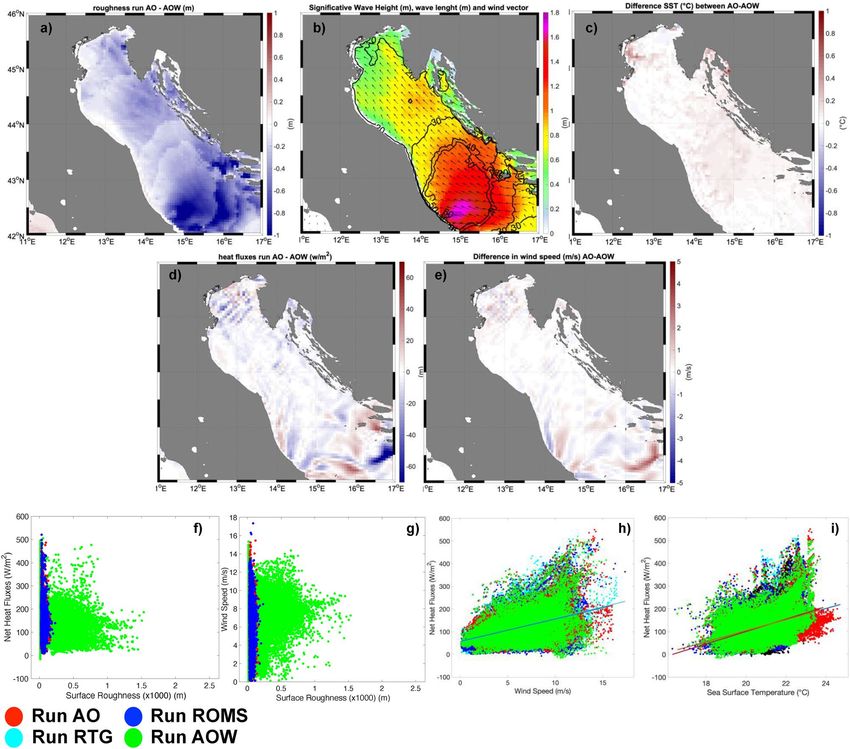
www.nature.com/scientificreports/
RUNS TYPE RTG ROMS SSTMOD FLAT MFS AO AOW AO3600 AOW3600
Homogeneous
Satellite (Mean Basin Operational Coupling Coupling Coupling Coupling
SST type SpinUp ROMS degraded
RTG_SST from ROMS Model WRF + ROMS WRF + ROMS + SWAN WRF + ROMS WRF + ROMS + SWAN
run)
SST source data
8.3 km 1 km 8.3 km / 4.5 km 1 km 1 km 1 km 1 km
resolution
SST upgrade 6h 6h 6h 6h 6h 600 s 600 s 3600 s 3600 s
Coupling No No No No No Yes Yes Yes Yes
Coupling fre-
/ / / / / 600 s 600 s 3600 s 3600 s
quency
Table 1. The table summarizes the types of runs proposed and the approaches followed in terms of type of Sea
Surface Temperature, resolution of the SST data, updating of the SST data and coupling.
Figure 2. Upper row: Sea Surface Temperature (SST) difference between the FLAT run and the other
simulations (in °C) at 06 UTC, September 26. Middle row: Surface Heat Fluxes difference between the FLAT run
and the other simulations (in W m−2). Bottom row: 10 m wind speed difference between the FLAT run and the
other simulations over sea surface. Due to the marked similarity in terms of SST with the AO run, the results for
AOW run are not shown here (see Fig. 3).
3) SSTMOD: SST is the same as that used in run ROMS, but at 8.3 km grid spacing. Thus, this run is intermedi-
ate between runs ROMS and RTG and its purpose is to evaluate the effect of resolution (in comparison with
ROMS) and of the data quality (in comparison with RTG);
4) FLAT: SST is uniform across the basin. The SST average value is calculated starting from run ROMS and
applied to the entire grid. It is designed to evaluate the influence of SST gradients and patterns on atmos-
pheric dynamics;
5) MFS: the SST is obtained from the CMEMS-MFS dataset29 at 4.5 km grid spacing, updated every 6 h. Con-
sequently the run MFS is similar to ROMS, but starts from a different modelling dataset, thus it is used to
estimate the impact of a different modelling dataset in comparison with the run ROMS.
In the second group, COAWST was used as a coupled numerical system. The initial conditions are the
result of the spin-up simulation.
6) AO: WRF and ROMS are 2-way coupled;
7) AOW: this is a fully coupled atmosphere–ocean–wave setup, envisaging the 2-way feedback of both atmos-
phere and ocean models with the wave model (SWAN), as described i n19,28;
Scientific Reports | (2021) 11:9388 | https://doi.org/10.1038/s41598-021-88476-1 4
Vol:.(1234567890)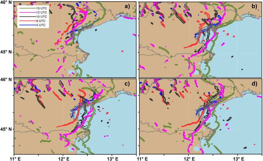
www.nature.com/scientificreports/
Figure 3. (a) Difference in surface roughness, (c) in SST, (d) in surface heat fluxes, (e) in 10 m wind speed
between run AO and run AOW, (b) significant height of the wave (shaded) and the peak length of the wave
fields (contours) in AOW run, (f) correlation between heat fluxes and surface roughness, (g) between heat fluxes
and surface roughness, (h) between heat fluxes and 10 m wind, (i) between heat fluxes and SST.
8) AO3600: this coupled run is identical to run AO, except for the coupling interval being 3600 s instead of
600 s;
9) AOW3600: same as in AOW, but with 3600 s as coupling interval.
Results
In order to compare the results from the different model setups, we first focus on the modelled SST field. The first
row in Fig. 2, which shows the differences in SST between the FLAT run and each model simulation at 06 UTC,
September 26 (shortly before the HPE) highlights significant differences in the northern and central Adriatic Sea.
The SST data obtained from satellite (RTG; Fig. 2a) is about 1.5 °C colder than the 1-km field (ROMS; Fig. 2b)
over the northern Adriatic Sea and along the Italian coast, while it is 1.5–2 °C warmer near the Croatian coast.
In semi-enclosed basins, particularly in rough coastal areas, satellites may be significantly affected by scattering
effects due to land and river plume contamination28, causing SST bias between 1 and 4 °C8,19.
The SST pattern in SSTMOD is similar to that of ROMS, but it misses the small-scale features, as a conse-
quence of the coarser resolution. Although the MFS and the ROMS run are both modelling outputs, significant
differences can be identified. These are not only due to the different resolution (4.5 km vs 1 km), but also to dif-
ferences in model formulation and input (e.g., freshwater sources) description. The differences are remarkable
in the area north-east of Ancona, where the two fields show respectively a cold and a warm plume extending
Scientific Reports | (2021) 11:9388 | https://doi.org/10.1038/s41598-021-88476-1 5
Vol.:(0123456789)www.nature.com/scientificreports/
from the Croatian coast, with differences up to 3 °C. The differences among the coupled runs (Fig. 3c) are more
limited, within a few tenths of 1 °C, mainly concentrated in the North Adriatic.
Comparing ROMS with the coupled approaches (Fig. 2b vs Fig. 2e), we note that the coupling induces a
different representation of the Po river plume, which is advected northward, thus leading to more mixed and
milder waters upstream of the convergence line (pink area in Fig. 2e). These differences can be partly attributed
to the different intervals of data communication (6 h in ROMS, 10 min in AO/AOW). Also, as shown in Fig. 3c,
the coupling with the waves in AOW induces a cooler SST, as a consequence of the stronger mixing28 of the river
water mass compared to AO. The areas with warmer SST induce greater (negative) surface heat fluxes (Fig. 2,
second row). As a consequence, in the northern Adriatic, in the area where the convergence line develops, the
sensible heat fluxes in ROMS and in the coupled runs can be up to 150 W m−2 higher than in the RTG and MFS
simulations, and 100 W m−2 than in the SSTMOD case. The warm temperature in the sub-basin in the ROMS
and AO fields is mainly associated with the Po river plume, which is hardly identified in satellite (RTG) and
low-resolution modelling data (MFS). In the northern Adriatic and in the central part of the basin, not only the
satellite SST (run RTG) is smaller than that in the coupled simulations (Fig. 2a vs Fig. 2e), but it is also associ-
ated with weaker winds (Fig. 2m vs Fig. 2q), up to 2.5 m/s. Such a difference in winds cannot be attributed to
differences in pressure patterns (Fig. SUPPL.2), increasing only after the frontal passage, but it is mainly due to
the different transfer of energy from the sea to the atmosphere, caused by the different SST values and patterns.
This is typical in areas of long fetch, after the wind has crossed hundreds of km in the same d irection30–36, such
as the northern Adriatic in this case study. Therefore, the wind intensity is modulated by the distribution of
the SST field, which influences the extraction of energy from the sea. Comparing the different coupled model
configurations, non-negligible differences are evident. Technically, the difference between the AO and AOW
runs lies in the addition of the wave model: waves transfer energy along the water column, increase the water
mixing37–39 and affect, through the wave roughness, the winds in the lowest meters of the a tmosphere40,41, thus
the drag coefficient and the heat fluxes from the sea surface. In the AO simulation, the WRF model imposes a
roughness calculated with C harnock42 scheme. In the AOW run the roughness is based on O ost43 parameteri-
zation (here preferred to other schemes available in COAWST), where the roughness depends on the wave age
(1996 ASGAMAGE experiment). Figure 3a shows that the AOW run generates greater roughness, in particular
in areas with greater significant height (Fig. 3b), e.g. the central Adriatic where waves are greater than 1.6 m and
the peak lengths about 50 m. In the other areas of the basin, roughness is only slightly greater in AOW runs. Fig-
ure 3c shows that the SST of the AO run is slightly warmer than that of the AOW run, in particular in the central
Adriatic and east of Venice, north of the Po river plume. The latter differences can be considered as a cumulative
effect of the water mixing associated with the waves in the downstream end of the basin in the AOW run, which
cools down the Po river plume as it is advected northward. Furthermore, the AO run produces, especially in the
North Adriatic, slightly higher wind speed U (about 0.1 m/ higher near the convergence line and 0.8 m/s east of
Venice; Fig. 3e and Table 1), due to the smaller roughness over the sea surface. However, despite the water cooling
and the overall lower wind speed (Fig. 3e), the AOW run shows more intense surface heat fluxes (Fig. 3d) in the
North Adriatic, due to the increase of both the roughness and drag coefficient. Figure 3f–i show that, differently
from the other runs, in the AOW run the surface roughness is a limiting factor for high wind intensity and SST,
but not for the heat fluxes. In contrast, the AO run produces higher SST values (Fig. 3i) and, due to the absence
of the wave-induced mixing, heat fluxes are mainly driven by the thermal forcing, while they are mainly guided
by surface roughness in AOW.
As expected, the aforementioned differences in air-sea interactions significantly affect the precipitation dis-
tribution. Figure 1 shows the precipitation amounts resulting from the different model configurations compared
with the data from the meteorological stations of the ARPAV network. The analysis of the precipitation simulated
in the different runs is based on the maximum 6-h accumulated precipitation (6–12 UTC) and on the average
distance (in km) between the simulated and the observed hourly maximum. Figure 1 shows that a more accurate
representation of the air-sea interaction processes leads to a more realistic rainfall amount and location. The rain-
fall amount ranges from 89 mm in run FLAT to more than 300 mm in the coupled runs, and the average distance
between the simulated and the observed storm ranges from 50 km (RTG) to about 30 km in the coupled runs.
Figure SUPPL3 clearly shows that the coupled runs outperform the standalone runs in terms of precipitation
amount and distribution. As discussed before, the different distribution of SST controls the energy fluxes between
the ocean and the atmosphere, affecting the wind fields. One might mistakenly think that this only happens
on the sea surface, but, in reality, there are differences simulated on a large scale and on the entire computing
domain. This leads us to conclude that there is a direct (thermal) component induced by the local interaction
between sea and atmosphere and an indirect one due to the different distribution of heat as the simulation pro-
gresses, affecting a wider area. Both AO and AOW coupled runs are able to simulate correctly the total amount
of precipitation (with a maximum value of about 340 mm and 325 mm respectively, while 360 mm have been
recorded in the station of Campagna Lupia). The coupled runs are the only ones able to reproduce the rainfall
along a stationary line extending from the Venetian lagoon northward. The location of the rainfall maximum in
AO and AOW runs is slightly shifted to the north-east of Campagna Lupia. By increasing the coupling interval
between models, similar results are observed in runs AO3600 and AOW3600 in terms of rainfall amount and
distance between the observed and the simulated cell (35 and 30 km). Figure 1e shows the Taylor diagram for all
the simulations, considering the time series of the maximum hourly accumulated rainfall (thus following the cell
evolution). Results show that the correlation (between 0.89 and 0.93) is high for all experiments, but the standard
deviation is much closer to the observations in the AO and AOW runs. The movement of the convergence line
obtained by different numerical runs is depicted in Fig. 4. This feature provides a dynamical perspective on the
difference in the spatial distribution of precipitation, which will be further discussed in “Discussion” section.
The structure of the storm is shown in Fig. 5, where modelled reflectivity fields are compared against radar
observations. Figure 5c–e and h–l show that the precipitation simulated in ROMS, AO and AOW runs develop
Scientific Reports | (2021) 11:9388 | https://doi.org/10.1038/s41598-021-88476-1 6
Vol:.(1234567890)www.nature.com/scientificreports/
Figure 4. Convergence line (0.003 s−1 isoline) location at 05, 08, 10, 12, 15 UTC on September 26, for run RTG
(a), ROMS (b), AO (c), and AOW (d).
Figure 5. Upper row: (a) 2-D radar reflectivity data (Vertical Maximum Intensity) in the HPE region;
synthetic radar data simulated in (b) RTG, (c) ROMS, (d) AO and (e) AOW; (f) cross section of the storm
radar reflectivity acquired by the radar in Teolo at 06 UTC, 26 September 2007; (g)–(l) reflectivity vertical
cross sections along the axes of most intense convection (whose locations are in panels (b)–(e) for (g) RTG, (h)
ROMS, (i) AO and (l) AOW.
from multiple cells arranged along the convergence line (north–south), in good agreement with the reflectivity
measured by ARPAV (Fig. 5a,f), while the RTG run (Figs. 4g and 5b) develops cells with lower reflectivity values
and shallower vertical development.
When we explore the reflectivity within the HPE region (Fig. 5a), the ROMS run (Fig. 5c) reproduces a storm
less intense compared to the coupled runs AO and AOW (Fig. 5d,e). In particular, the coupled runs are able to
Scientific Reports | (2021) 11:9388 | https://doi.org/10.1038/s41598-021-88476-1 7
Vol.:(0123456789)www.nature.com/scientificreports/
RTG ROMS AO AOW FLAT SSTMOD MFS
U (m/s) 10.3 12.2 11.7 11.6 10.5 11.4 12.0
LFC (m) 615 591 575 593 502 506 780
N (10−2 s−1) 1.4 1.1 1.1 1.1 1.1 1.2 1.2
h (m) 400 600 700 700 150 500 600
h/LFC 0.65 1.02 1.22 1.18 0.29 0.98 0.76
Cs (m/s) 9.0 11.0 12.0 12.0 8.0 10.2 11.0
Table 2. Meteorological fields averaged in the rectangular box 45°–45.5°N and 12.5°–13°E evaluated at 09
UTC of 26 September 2007, during the most intense part of the event.
reproduce the V-shaped structure of the storm at the right location with the proper intensity (Fig. 5e). Also, in
terms of reflectivity field, the AO and AOW runs show values and spatial patterns comparable with the radar
data. Satellite observations highlight the presence of possible overshooting t ops15, which are consistent with the
high cloud tops (at about 11 km) simulated in the ROMS and coupled runs (Fig. 5h–l).
Discussion
Operational NWP models were not able to properly simulate the rainfall amount and location of the analyzed
HPE, therefore missing their function of alerting the local authorities about the exceptional amount of rain to
be expected. The analysis of different Limited Area Model (LAM) simulations15 highlighted a large variability
depending on the large scale forcing, on the model formulation, and on the time of initialization. Our results
show that the explicit and consistent description of the air-sea interactions leads to a noticeable improvement in
the model skills. However, in order to clearly understand why this result is achieved, we need to summarise the
state of the atmospheric system with a limited number of bulk parameters. To this aim, the quantities describ-
ing the average dynamical and thermodynamic properties immediately upstream of the event are shown in
Table 2. In particular, the presence or absence of favorable conditions for intense, localized and quasi-stationary
convection is assessed.
First, the environmental wind speed U is smaller in the RTG run than in the other simulations. This is a
direct consequence of the changes induced by the difference in SST, which, in the RTG run, is cooler on the
northern and western Adriatic coast, and warmer along the Croatian coast. This modifies the circulation not
only over the sea surface, but also near the coasts, in the areas most exposed to the incoming moist and warm
flow from the Adriatic Sea, up to the Pre-Alpine ridge. There, the environmental flow in the RTG run is more
westward-oriented than in the other simulations, producing a wider but shallower extension of cold air barrier
flow extending from the Alps (not shown).
Second, in the RTG case the environmental profile is less favorable to the triggering of convection, due to
the higher level of free convection (LFC) and to the greater Brunt-Väisälä frequency (N). In fact, while the latter
indicates a higher resistance of the environment to vertical displacements, the former denotes a weaker tendency
of the low-level parcels to reach LFC and trigger convection. This tendency is represented by the nondimensional
parameter h/LFC44,45 where, following46, h does not represent the mountain height but the height of the cold
pool, which behaves as an obstacle to the incoming southerly flow. In Table 2, h is evaluated as approximately
equal to the height of the 1 °C potential temperature anomaly. The shallower vertical extension h of the cold
pool and the higher LFC in the RTG experiment imply a value of h/LFC smaller than those observed in ROMS
and in the coupled experiments, indicating weaker vertical displacement and tendency to convection. Figure 5
clearly shows that convection is much shallower and less intense in the RTG run compared to the coupled runs.
After this analysis, we go back to Fig. 4 and investigate more in details why the convergence line remains
quasi-stationary in the coupled runs (Fig. 4c,d), while it changes significantly in the RTG experiment (Fig. 4a).
This point is relevant considering that a stationary convergence line implies persistent convective triggering
and rainfall in the same area. To identify if these conditions occur, here we follow the analysis performed by
Miglietta and R otunno47 and compare the theoretical cold pool propagation speed Cs, associated with the cold
air that has remained confined in the low-level (whose vertical extension is given by h), with the environmental
wind U, evaluated in the rectangle located offshore (in latitude 45 °N–45.4 °N and longitude 12.5 °E–13.3 °E,
based on Davolio et al.15), representative of the warm and moist air moving from the Adriatic toward the cold
pool. We checked that Cs and U have approximately opposite direction in all cases. Assuming that the cold-pool
48 49
behaves as a density current, B
enjamin and
K lemp estimated the propagation speed as: Cs = 2g ′ h , where
g = g(θ1 − θ0 )/θ0, being θ1 the potential temperature of the environment and θ0 that of the cold air mass. In
′
RTG and ROMS runs, Cs is smaller than the environmental wind U at 06 UTC (see Table 2) so that the cold
pool penetrates inland. On the other hand, in the coupled simulations Cs is higher than in RTG because of the
higher depth h. The wind speed U also increases with respect to RTG, but not as much as Cs, so that the cold pool
propagation is approximately counteracted by the environmental wind. The balance between these two flows
represents the most favorable conditions for rainfall accumulation, as the uplift induced by convergence may
remain stationary in the same position for several h ours47.
Scientific Reports | (2021) 11:9388 | https://doi.org/10.1038/s41598-021-88476-1 8
Vol:.(1234567890)www.nature.com/scientificreports/
Conclusions
In coastal areas a detailed description of SST distribution plays a fundamental role for an accurate assessment of
the MABL energy budget, with relevant implication for rainfall p rediction50. However, despite new techniques
of satellite acquisition, it is still difficult to get accurate SST data in coastal areas, in particular during extensive
periods of cloud coverage.
This paper presents a numerical study using a high-resolution fully-coupled atmosphere–ocean–wave regional
modelling system to analyze the sensitivity of an early Fall HPE in the surrounding of Venice. Compared to
standalone atmospheric simulations using satellite data (run RTG), where the SST is available at coarse resolu-
tion every 6 h, and other SST datasets of different origin and resolution, the coupled systems AO and AOW
provide significantly improved results in terms of precipitation amount, location, and timing of evolution. This
is a consequence of the better representation of the fine-scale SST patterns due to the consistent treatment of
air-sea interaction processes12,28. Therefore, the convergence of different air masses (cold, dry air from the Alpine
regions and moist, warm air from the Adriatic basin), which is responsible for the generation of a back-building
convective system, is better reproduced. Differences appear also comparing ROMS, where SST is updated at
high-resolution, and AO/AOW cases, as only in the latter runs the heat fluxes at the MABL were consistently
computed by the fully coupled system.
Also, as shown in Prtenjak50, 50% of summer days along the northern Adriatic coast are characterized by the
presence of land-sea breeze systems. They usually develop between 08 and 18 UTC50, reaching their maximum
intensity at around 15 UTC. In a semi-enclosed basin, such as the North Adriatic, during late summer the effect
induced by breeze components may represent a secondary forcing for HPEs, which may locally add up to the
main process, i.e. the large-scale dynamics. However, sea breeze may also contribute to the development of con-
vection due to convergence with other breeze s ystems51,52, fronts, cold pools associated with previous precipita-
tion, etc. The breeze dynamics are also influenced by the distribution of SST, which may locally affect the location
of the coastal convergence l ine53,54. In this complex context, coupled atmosphere–ocean models, implementing
high-resolution and frequently updated SSTs, represent more realistically coastal dynamics. Further studies are,
however, needed to better assess their application to this phenomenology.
This study provides clear indications that the accurate simulation of localized rainfall events is eventually the
result of a delicate interplay of energy balance that needs to be properly accounted for. A slight adjustment of
the wind field, which may be provided by the different heat distribution along the coast generated by an ocean
circulation model, can indeed change significantly the amount and location of forecast rainfall. In the same way,
stormy conditions may enhance the role of surface waves in affecting momentum across the M ABL28. Although
limited to one case study, results presented here have a general value, on the one hand about the relevance of the
use of model coupling and, on the other hand, about the limitations of operational NWP approaches when con-
stant or coarse resolution SSTs are used as surface boundary conditions. The Mediterranean region is frequently
affected by HPEs, often related to the presence of convergence lines55,56, which are associated to the clashing of
cold and dry air versus highly-unstable, warm and moist masses. In our case study, the use of high resolution and
frequently updated SST improved the timing performance of the convergence line (well depicted by ROMS, AO
and AOW runs), thus allowing a better simulation of the rainfall amount and location. Having said this, in order
to provide improved HPE and hazard predictions in other coastal regions via coupled numerical tools, there is
still a strong need to explore a broad range of conditions, as well as to carry out more extensive sensitivity studies.
Data availability
The datasets generated and/or analysed during the current study are available from the corresponding author
on reasonable request.
Received: 19 September 2018; Accepted: 22 March 2021
References
1. Cassola, F., Ferrari, F., Mazzino, A. & Miglietta, M. M. The role of the sea on the flash floods events over Liguria (northwestern
Italy). Geophys. Res. Lett. 43(7), 3534–3542. https://doi.org/10.1002/2016GL068265 (2016).
2. Meroni, A. N., Parodi, A. & Pasquero, C. Role of SST patterns on surface wind modulation of a heavy midlatitude precipitation
event. J. Geophys. Res. Atmos. 123, 9081–9096. https://doi.org/10.1029/2018JD028276 (2018).
3. Duffourg, F. & Ducrocq, V. Origin of the moisture feeding the heavy precipitating systems over Southeastern France. Hazards
Earth Syst. Sci. 11, 1163–1178. https://doi.org/10.5194/nhess-11-1163-2011 (2011).
4. Berthou, S. et al. Sensitivity of an intense rain event between atmosphere-only and atmosphere-ocean regional coupled models:
19 September 1996. Q. J. R. Meteorol. Soc. 141(686), 258–271. https://doi.org/10.1002/qj.2355 (2015).
5. LebeaupinBrossier, C. et al. Ocean mixed layer responses to intense meteorological events during HyMeX-SOP1 from a high-
resolution ocean simulation. Ocean Model 84, 84–103. https://doi.org/10.1016/J.OCEMOD.2014.09.009 (2014).
6. Pastor, F., Valiente, J. A. & Estrela, M. J. Sea surface temperature and torrential rains in the Valencia region: modelling the role of
recharge areas. Hazards Earth Syst. Sci 15, 1677–1693. https://doi.org/10.5194/nhess-15-1677-2015 (2015).
7. Fiori, E. et al. Analysis and hindcast simulations of an extreme rainfall event in the Mediterranean area: the Genoa 2011 case.
Atmos. Res. 138, 13–29. https://doi.org/10.1016/J.ATMOSRES.2013.10.007 (2014).
8. Davolio, S. et al. Effects of increasing horizontal resolution in a convection-permitting model on flood forecasting: the 2011 dra-
matic events in Liguria, Italy. J. Hydrometeorol. 16(4), 1843–1856. https://doi.org/10.1175/JHM-D-14-0094.1 (2015).
9. Miglietta, M. M. et al. Numerical analysis of a Mediterranean “hurricane” over south-eastern Italy: sensitivity experiments to sea
surface temperature. Atmos. Res. 101(1–2), 412–426. https://doi.org/10.1016/J.ATMOSRES.2011.04.006 (2011).
10. Ricchi, A. et al. Sensitivity of a mediterranean tropical-like cyclone to different model configurations and coupling strategies.
Atmosphere 8(12), 92. https://doi.org/10.3390/atmos8050092 (2017).
11. Miglietta, M. M., Mazon, J., Motola, V. & Pasini, A. Effect of a positive sea surface temperature anomaly on a Mediterranean
tornadic supercell. Sci. Rep. 7(12828), 1–8. https://doi.org/10.1038/s41598-017-13170-0 (2017).
Scientific Reports | (2021) 11:9388 | https://doi.org/10.1038/s41598-021-88476-1 9
Vol.:(0123456789)www.nature.com/scientificreports/
12. Lewis, H. W. et al. The UKC2 regional coupled environmental prediction system. Geosci. Model Dev. 11, 1–42. https://doi.org/10.
5194/gmd-11-1-2018 (2018).
13. Rossa, A. M., Laudanna Del Guerra, F., Zanon, F., Settin, T. & Leuenberger, D. Radar-driven high-resolution hydro-meteorological
forecasts of the 26 September 2007 Venice flash flood. J. Hydrol. 394(1–2), 230–244. https://doi.org/10.1016/J.JHYDROL.2010.08.
035 (2010).
14. Barbi, A., Monai, M., Racca, R. & Rossa, A. M. Recurring features of extreme autumn all rainfall events on the Veneto coastal area.
Hazards Earth Syst. Sci. 12, 2463–2477. https://doi.org/10.5194/nhess-12-2463-2012 (2012).
15. Davolio, S. et al. High resolution simulations of a flash flood near Venice. Nat. Hazards Earth Syst. Sci. 9(5), 1671–1678. https://
doi.org/10.5194/nhess-9-1671-2009 (2009).
16. McCann, D. W. & McCann, D. W. The enhanced-V: a satellite observable severe storm signature. Mon. Weather Rev. 111(4),
887–894. https://doi.org/10.1175/1520-0493(1983)111%3c0887:TEVASO%3e2.0.CO;2 (1983).
17. Warner, J. C., Armstrong, B., He, R. & Zambon, J. B. Development of a coupled ocean–atmosphere–wave–sediment transport
(COAWST) modeling system. Ocean Model 35(3), 230–244. https://doi.org/10.1016/J.OCEMOD.2010.07.010 (2010).
18. Olabarrieta, M., Warner, J. C., Armstrong, B., Zambon, J. B. & He, R. Ocean–atmosphere dynamics during Hurricane Ida and
Nor’Ida: An application of the coupled ocean–atmosphere–wave–sediment transport (COAWST) modeling system. Ocean Model
43–44, 112–137. https://doi.org/10.1016/J.OCEMOD.2011.12.008 (2012).
19. Ricchi, A. et al. On the use of a coupled ocean–atmosphere–wave model during an extreme cold air outbreak over the Adriatic
Sea. Atmos. Res. 172–173, 48–65. https://doi.org/10.1016/J.ATMOSRES.2015.12.023 (2016).
20. Skamarock, W. C. & Klemp, J. B. A time-split nonhydrostatic atmospheric model for weather research and forecasting applications.
J. Comput. Phys. 227, 3465–3485. https://doi.org/10.1016/j.jcp.2007.01.037 (2008).
21. Shchepetkin, A. F. & McWilliams, J. C. The regional oceanic modeling system (ROMS): a split-explicit, free-surface, topography-
following-coordinate oceanic model. Ocean Model 9, 347–404. https://doi.org/10.1016/j.ocemod.2004.08.002 (2005).
22. Booij, N., Ris, R. C. & Holthuijsen, L. H. A third-generation wave model for coastal regions: 1. Model description and validation.
J. Geophys. Res. Ocean. 104, 7649–7666. https://doi.org/10.1029/98JC02622 (1999).
23. Kain, J. S. & Kain, J. S. The Kain–Fritsch convective parameterization: an update. J. Appl. Meteorol. 43(1), 170–181. https://doi.
org/10.1175/1520-0450(2004)043%3c0170:TKCPAU%3e2.0.CO;2 (2004).
24. Hong, S.-Y. et al. A revised approach to ice microphysical processes for the bulk parameterization of clouds and precipitation.
Mon. Weather Rev. 132(1), 103–120. https://doi.org/10.1175/1520-0493(2004)132%3c0103:ARATIM%3e2.0.CO;2 (2004).
25. Janjic, Z. I. The step-mountain eta coordinate model: further developments of the convection, viscous sublayer, and turbulence
closure schemes. Mon. Weather Rev. https://doi.org/10.1175/1520-0493(1994)122%3c0927:TSMECM%3e2.0CO:2 (1994).
26. Mlawer, E. J., Taubman, S. J., Brown, P. D., Iacono, M. J. & Clough, S. A. Radiative transfer for inhomogeneous atmospheres: RRTM,
a validated correlated-k model for the longwave. J. Geophys. Res. Atmos. 102(D14), 16663–16682. https://doi.org/10.1029/97JD0
0237 (1997).
27. Benetazzo, A. et al. Response of the Adriatic Sea to an intense cold air outbreak: dense water dynamics and wave-induced transport.
Prog. Oceanogr. 128, 115–138. https://doi.org/10.1016/J.POCEAN.2014.08.015 (2014).
28. Carniel, S. et al. Scratching beneath the surface while coupling atmosphere, ocean and waves: analysis of a dense water formation
event. Ocean Model 101, 101–112. https://doi.org/10.1016/J.OCEMOD.2016.03.007 (2016).
29. Pinardi, N. et al. The Mediterranean ocean forecasting system: first phase of implementation (1998–2001). Ann. Geophys. 21(1),
3–20 (2002).
30. O’Neill, L. W. et al. Observations of SST-induced perturbations of the wind stress field over the Southern Ocean on seasonal
timescales. J. Clim. 16(14), 2340–2354. https://doi.org/10.1175/2780.1 (2003).
31. O’Neill, L. W. et al. High-resolution satellite measurements of the atmospheric boundary layer response to SST variations along
the Agulhas return current. J. Clim. 18(14), 2706–2723. https://doi.org/10.1175/JCLI3415.1 (2005).
32. O’Neill, L. W. et al. The effects of SST-induced surface wind speed and direction gradients on midlatitude surface vorticity and
divergence. J. Clim. 23(2), 255–281. https://doi.org/10.1175/2009JCLI2613.1 (2010).
33. Chelton, D. B. & Chelton, D. B. The impact of SST specification on ECMWF surface wind stress fields in the Eastern Tropical
Pacific. J. Clim. 18(4), 530–550. https://doi.org/10.1175/JCLI-3275.1 (2005).
34. Chelton, D. B. et al. Observations of coupling between surface wind stress and sea surface temperature in the Eastern Tropical
Pacific. J. Clim. 14(7), 1479–1498. https://doi.org/10.1175/1520-0442(2001)014%3c1479:OOCBSW%3e2.0.CO;2 (2001).
35. Chelton, D. B. et al. Summertime coupling between sea surface temperature and wind stress in the California current system. J.
Phys. Oceanogr. 37(3), 495–517. https://doi.org/10.1175/JPO3025.1 (2007).
36. Obermann, A., Edelmann, B. & Ahrens, B. Influence of sea surface roughness length parameterization on Mistral and Tramontane
simulations. Adv. Sci. Res. 13, 107–112. https://doi.org/10.5194/asr-13-107-2016 (2016).
37. Benetazzo, A., Carniel, S., Sclavo, M. & Bergamasco, A. Wave–current interaction: effect on the wave field in a semi-enclosed basin.
Ocean Model 70, 152–165. https://doi.org/10.1016/J.OCEMOD.2012.12.009 (2013).
38. McWilliams, J. C. & Fox-Kemper, B. Oceanic wave-balance surface fronts and filaments. J. Fluid Mech. 730, 464–490. https://doi.
org/10.1017/jfm.2013.348 (2013).
39. McWilliams, J. C., Huckle, E., Liang, J.-H. & Sullivan, P. P. 2012: the wavy Ekman layer: Langmuir circulations, breaking waves,
and Reynolds stress. J. Phys. Oceanogr. 42, 1793–1816. https://doi.org/10.1175/JPO-D-12-07.1 (2002).
40. Zhang, L. et al. Impact of sea spray on the yellow and East China Seas thermal structure during the passage of typhoon rammasun.
J. Geophys. Res. Oceans https://doi.org/10.1002/2016JC012592 (2017).
41. Zhang, X. et al. Effect of surface wave breaking on the surface boundary layer of temperature in the Yellow Sea in summer. Ocean
Model 38(3), 267–279. https://doi.org/10.1016/j.ocemod.2011.04.006 (2011).
42. Charnock, H. Wind stress on a water surface. Q. J. R. Meteorol. Soc. 81, 639–640. https://doi.org/10.1002/qj.49708135027(1955)
(1955).
43. Oost, W. A., Komen, G. J., Jacobs, C. M. J. & Van Oort, C. New evidence for a relation between wind stress and wave age from
measurements during ASGAMAGE. Bound. Layer Meteorol. 103, 409–438. https://doi.org/10.1023/A:1014913624535 (2002).
44. Miglietta, M. M. & Rotunno, R. Numerical simulations of conditionally unstable flows over a mountain ridge. J. Atmos. Sci. 66(7),
1865–1885. https://doi.org/10.1175/2009JAS2902.1 (2009).
45. Miglietta, M. M. & Rotunno, R. Numerical simulations of low-CAPE flows over a mountain ridge. J. Atmos. Sci. 67(7), 2391–2401.
https://doi.org/10.1175/2010JAS3378.1 (2010).
46. Davolio, S. et al. Mechanisms producing different precipitation patterns over north-eastern Italy: insights from HyMeX-SOP1 and
previous events. Q. J. R. Meteorol. Soc. 142, 188–205. https://doi.org/10.1002/qj.2731 (2016).
47. Miglietta, M. M. & Rotunno, R. Numerical simulations of sheared conditionally unstable flows over a mountain ridge. J. Atmos.
Sci. 71(5), 1747–1762. https://doi.org/10.1175/JAS-D-13-0297.1 (2014).
48. Benjamin, T. Gravity currents and related phenomena. J. Fluid Mech. 31(2), 209–248. https://doi.org/10.1017/S00221120680001
33 (1968).
49. Klemp, J. B., Rotunno, R. & Skamarock, W. C. On the dynamics of gravity currents in a channel. J. Fluid Mech. 269(1), 169. https://
doi.org/10.1017/S0022112094001527 (1994).
50. Prtenjak, M. T. & Grisogono, B. Sea/land breeze climatological characteristics along the northern Croatian Adriatic coast. Theor.
Appl. Climatol. 90, 201–215. https://doi.org/10.1007/s00704-006-0286-9 (2007).
Scientific Reports | (2021) 11:9388 | https://doi.org/10.1038/s41598-021-88476-1 10
Vol:.(1234567890)www.nature.com/scientificreports/
51. Mangia, C., Martano, P., Miglietta, M. M., Morabito, A. & Tanzarella, A. Modelling local winds over the Salento peninsula. Met.
Apps 11, 231–244. https://doi.org/10.1017/S135048270400132X (2004).
52. Comin, A. N., Miglietta, M. M., Rizza, U., Costa, O. & Annes, G. Investigation of sea breeze convergence in Salento Peninsula
(southeastern Italy). Atmos. Res. 160, 68–79. https://doi.org/10.1016/j.atmosres.2015.03.010 (2015).
53. Shi, R., Cai, Q., Dong, L., Guo, X. & Wang, D. Response of the diurnal cycle of summer rainfall to large-scale circulation and coastal
upwelling at Hainan, South China. J. Geophys. Res. Atmos. 124, 3702–3725. https://doi.org/10.1029/2018JD029528 (2019).
54. Kilpatrick, T., Xie, S.-P. & Nasuno, T. Diurnal convection-wind coupling in the Bay of Bengal. J. Geophys. Res. Atmos. 122,
9705–9720. https://doi.org/10.1002/2017JD027271 (2017).
55. Lee, K.-O. et al. HAL Id: insu-01327507 https://hal-insu.archives-ouvertes.fr/insu-01327507 Convective initiation and mainte-
nance processes of two back-building mesoscale convective systems leading to heavy precipitation events in Southern Italy during
HyMeX IOP 13 Convective initiation and maintenance processes of two back-building mesoscale convective systems leading to
heavy precipitation events in Southern Italy during HyMeX IOP 13. Q. J. R. Meteorol. Soc. https://doi.org/10.1002/qj.2851 (2016).
56. Mastrangelo, D., Horvath, K., Riccio, A. & Miglietta, M. M. Mechanisms for convection development in a long-lasting heavy pre-
cipitation event over southeastern Italy. Atmos. Res. 100(4), 586–602. https://doi.org/10.1016/J.ATMOSRES.2010.10.010 (2011).
Acknowledgements
The work was partially supported by the H2020 project CEASELESS number 730030 and Grant CINECA
“COMOLF” number HP10C2SECI. Antonio Ricchi funding have been provided via the PON “AIM” linea 2 -
Attraction and international mobility program AIM1858058. Our thanks goes to Veneto Region Environmental
Protection Agency (ARPAV) for providing meteorological stations and radar data.
Author contributions
A.R. conceived the study, A.R. and M.M.M. contributed in numerical model setup; D.B., G.C. M.M.M and S.C.
analysed the results. All authors wrote and reviewed the manuscript.
Competing interests
The authors declare no competing interests.
Additional information
Supplementary Information The online version contains supplementary material available at https://doi.org/
10.1038/s41598-021-88476-1.
Correspondence and requests for materials should be addressed to A.R.
Reprints and permissions information is available at www.nature.com/reprints.
Publisher’s note Springer Nature remains neutral with regard to jurisdictional claims in published maps and
institutional affiliations.
Open Access This article is licensed under a Creative Commons Attribution 4.0 International
License, which permits use, sharing, adaptation, distribution and reproduction in any medium or
format, as long as you give appropriate credit to the original author(s) and the source, provide a link to the
Creative Commons licence, and indicate if changes were made. The images or other third party material in this
article are included in the article’s Creative Commons licence, unless indicated otherwise in a credit line to the
material. If material is not included in the article’s Creative Commons licence and your intended use is not
permitted by statutory regulation or exceeds the permitted use, you will need to obtain permission directly from
the copyright holder. To view a copy of this licence, visit http://creativecommons.org/licenses/by/4.0/.
© The Author(s) 2021
Scientific Reports | (2021) 11:9388 | https://doi.org/10.1038/s41598-021-88476-1 11
Vol.:(0123456789)You can also read