Simulation of the soil water balance of wheat using daily weather forecast messages to estimate the reference evapotranspiration
←
→
Page content transcription
If your browser does not render page correctly, please read the page content below
Hydrol. Earth Syst. Sci., 13, 1045–1059, 2009
www.hydrol-earth-syst-sci.net/13/1045/2009/                                                          Hydrology and
© Author(s) 2009. This work is distributed under                                                      Earth System
the Creative Commons Attribution 3.0 License.                                                             Sciences

Simulation of the soil water balance of wheat using daily weather
forecast messages to estimate the reference evapotranspiration
J. B. Cai1 , Y. Liu1 , D. Xu1 , P. Paredes2 , and L. S. Pereira2
1 Departmentof Irrigation and Drainage, China Inst. of Water Resources and Hydropower Research, Beijing 100044, China
2 Agricultural
            Engineering Research Center, Inst. of Agronomy, Technical University of Lisbon, Tapada da Ajuda,
1349-017 Lisbon, Portugal
Received: 16 December 2008 – Published in Hydrol. Earth Syst. Sci. Discuss.: 5 February 2009
Revised: 11 May 2009 – Accepted: 25 June 2009 – Published: 9 July 2009

Abstract. Aiming at developing real time water balance             1   Introduction
modelling for irrigation scheduling, this study assesses the
accuracy of using the reference evapotranspiration (ETo ) es-      Recent developments in irrigation management consist in
timated from daily weather forecast messages (ETo,WF ) as          tools to support real-time irrigation decision-making. Their
model input. A previous study applied to eight locations in        adoption requires that appropriate weather data are avail-
China (Cai et al., 2007) has shown the feasibility for esti-       able to perform soil water balance computations for accu-
mating ETo,WF with the FAO Penman-Monteith equation us-            rately determine the timing and volumes of irrigation. Real-
ing daily forecasts of maximum and minimum temperature,            time irrigation scheduling has proved appropriate when us-
cloudiness and wind speed. In this study, the global radiation     ing weather data forecasts provided by commercial services
is estimated from the difference between the forecasted max-       to estimate the reference evapotranspiration (ETo ). Applica-
imum and minimum temperatures, the actual vapour pres-             tions are reported for several crops such as potato (Gowing
sure is estimated from the forecasted minimum temperature          and Ejieji, 2001), lettuce (Wilks and Wolfe, 1998) and maize
and the wind speed is obtained from converting the com-            (Cabelguenne et al., 1997). In alternative to weather data
mon wind scales into wind speed. The present application           forecasts, generated weather data produced by a climatic data
refers to a location in the North China Plain, Daxing, for the     generator may also be used (Donatelli et al., 2003; Stöckle et
wheat crop seasons of 2005–2006 and 2006–2007. Results             al., 2003, 2004).
comparing ETo,WF with ETo computed with observed data                 Another approach to real-time irrigation scheduling con-
(ETo,obs ) have shown favourable goodness of fitting indica-       sists of deriving actual crop coefficients (Kc ) from remote
tors and a RMSE of 0.77 mm d−1 . ETo was underestimated            sensing and using ground and satellite weather data to esti-
in the first year and overestimated in the second. The wa-         mate the actual crop evapotranspiration (ETc ) for determin-
ter balance model ISAREG was calibrated with data from             ing irrigation requirements. Various applications and mod-
four treatments for the first season and validated with data of    elling approaches are reported with applications for estima-
five treatments in the second season using observed weather        tion of actual ETc at regional or irrigation system scales
data. The calibrated crop parameters were used in the simu-        (Ray and Dadhwal, 2001; Consoli et al., 2006; Tasumi and
lations of the same treatments using ETo,WF as model input.        Allen, 2007). At the field scale, Hunsaker et al. (2005) devel-
Errors in predicting the soil water content are small, 0.010       oped a model for determining wheat basal crop coefficients
and 0.012 m3 m−3 , respectively for the first and second year.     from observations of the normalized difference vegetation
Other indicators also confirm the goodness of model predic-        index (NDVI) and to estimate wheat evapotranspiration us-
tions. It could be concluded that using ETo computed from          ing the FAO-56 procedures. Chavez et al. (2008) computed
daily weather forecast messages provides for accurate model        daily ETc from instantaneous latent heat flux estimates de-
predictions and to use an irrigation scheduling model in real      rived from digital airborne multispectral remote sensing im-
time.                                                              agery. Reviews are presented by Courault et al. (2005) and
                                                                   Gowda et al. (2008). Applications aiming at using crop co-
                                                                   efficients estimated from remote sensing for supporting irri-
                     Correspondence to: L. S. Pereira              gation scheduling have been reported recently (Calera Bel-
                     (lspereira@isa.utl.pt)                        monte et al., 2005; Garatuza-Payan and Watts, 2005; Santos

Published by Copernicus Publications on behalf of the European Geosciences Union.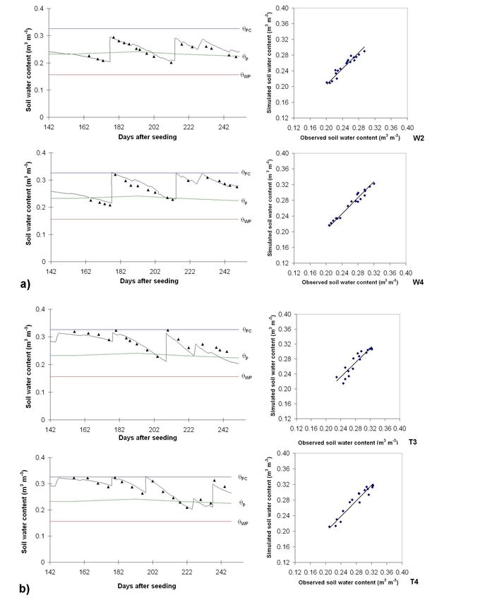
1046                                                                        J. B. Cai et al.: Water balance with weather forecasts

et al., 2008). The mentioned applications refer to large fields;   referred hereafter as ETo,obs ; the other consisting of weather
when small fields (0.1–0.5 ha) are considered, as it is the case   forecast messages from the public media, which estimated
in China, the use of remote sensing data is not appropriate        daily values are referred as ETo,WF .
due to pixel size limitations.                                        The daily ETo (mm d−1 ) was computed with the PM-ETo
   To develop real-time irrigation management for North            equation (Allen et al., 1998):
China, a different approach was developed by combining                                          900
                                                                           0.4081 (Rn −G) + γ T +273 u2 (es −ea )
weather data forecast messages produced by the China Mete-         ETo =                                                       (1)
orological Administration with an irrigation scheduling sim-                        1 + γ (1 + 0.34u2 )
ulation model. This approach allows to determine in real-          where Rn is the net radiation at the crop surface
time both the crop evapotranspiration (ETc ) and the available     (MJ m−2 d−1 ), G is soil heat flux density (MJ m−2 d−1 ), T is
soil water, thus to determine when and how much to irrigate.       the air temperature at 2 m height (◦ C), u2 is the wind speed
   The FAO Penman-Monteith reference evapotranspiration            at 2 m height (m s−1 ), es is the vapour pressure of the air at
(PM-ETo) equation (Allen et al., 1998) is worldwide adopted        saturation (kPa), ea is the actual vapour pressure (kPa), 1 is
as the standard method to compute ETo from meteorologi-            the slope of the vapour pressure curve (kPa ◦ C−1 ), and γ is
cal data. Its computation requires weather data on maximum         the psychrometric constant (kPa ◦ C−1 ). G may be ignored
and minimum temperature (Tmax and Tmin ), solar radiation          for daily time step computations.
(Rs ), relative humidity (RH) and wind speed at 2 m height            The ETo estimation procedure using WF data (Cai et al.,
(u2 ). Alternative calculation procedures proposed by Allen        2007) consists of estimating the parameters of Eq. (1) from
et al. (1998) to be adopted when not all these data are avail-     the weather forecast messages using daily maximum and
able were tested and validated in China (Liu and Pereira,          minimum air temperatures, wind grade and weather condi-
2001; Pereira et al., 2003a) and elsewhere (Popova et al.,         tions (such as sunny, cloudy, rainy). The forecasted values of
2006b; Jabloun and Sahli, 2008).                                   Tmax and Tmin (◦ C) are used similarly to the observed ones
   Considering that good results were obtained for North           in ETo computations. The daily actual vapour pressure (ea )
China using those alternative procedures, a new analytic           is estimated from the forecasted daily Tmin adopting the fol-
methodology for computing the PM-ETo equation using                lowing equation (Allen et al, 1998):
weather forecast messages (WF) has been developed (Cai et
                                                                                                    17.27Tmin

                                                                           0
al., 2007). It was tested for several locations in China at dif-   ea = e (Tmin ) = 0.611 exp                                  (2)
                                                                                                   Tmin + 237.3
ferent latitudes and longitudes representing various climates.
ETo estimated with WF data can thus be used as input to a          where ea is the actual vapour pressure (kPa) and eo (Tmin ) is
simulation model for real-time irrigation scheduling. Testing      the saturation vapour pressure at Tmin .
this approach using the model ISAREG, which has been pre-             In the former study (Cai et al., 2007), the global radi-
viously calibrated and validated in North China (Liu et al.,       ation Rs (MJ m−2 d−1 ) was estimated from the forecasted
1998, 2006), constitutes the main objective of this research.      “weather condition” referring to five cloudiness conditions:
This research shall be further continued to spatialize both the    clear sky, clear to cloudy, cloudy, overcast and rainy. The
WF data and model outputs to be used at project, basin or          actual duration of sunshine hours n was then estimated from
region level with several of crops.                                the day time duration N as n=aN, where the parameter a as-
   The purpose of this paper is to examine the accuracy of         sumed the values 0.9, 0.7, 0.5, 0.3 and 0.1 respectively for the
using the WF estimates of ETo (ETo,WF ) for a non-synoptic         five cloudiness conditions referred above. Then Rs was com-
location when compared with those obtained when the PM-            puted with the Angström equation (Angström, 1924). How-
ETo equation is used with observed weather data (ETo,obs ).        ever, considering the good results obtained for the estima-
The paper includes the calibration and validation of the           tion of Rs from the difference Tmax −Tmin (Liu and Pereira,
model using observations of the soil water content, as well        2001; Pereira et al., 2003a; Popova et al., 2006b; Jabloun and
as the comparison of results of the same model when ETo,WF         Sahli, 2008), the above mentioned procedure was replaced in
and ETo,obs are used as model inputs. The application refers       this study by the Hargreaves’ radiation equation modified by
to various irrigation treatments of a wheat crop at Daxing, in     Allen et al. (1998):
the North China Plain.                                             Rs = kRs (Tmax − Tmin )0.5 Ra                               (3)
                                                                   where kRs is the adjustment coefficient (◦ C−0.5 ), and Ra is
2     Material and methods                                         the radiation on top of the atmosphere (MJ m−2 d−1 ). kRs
                                                                   is empirical and differs for “interior” or “coastal” regions.
2.1    Reference ET estimations                                    For “interior” locations, where land mass dominates and air
                                                                   masses are not strongly influenced by a large water body,
For the purpose of this study, two sets of weather data were       kRs ≈0.17. This value has been previously tested for the re-
used to estimate ETo : one using hourly observations from          gion (Pereira et al., 1998; Liu and Pereira, 2001; Pereira et
a nearby weather station, which computed daily values are          al., 2003a).

Hydrol. Earth Syst. Sci., 13, 1045–1059, 2009                                      www.hydrol-earth-syst-sci.net/13/1045/2009/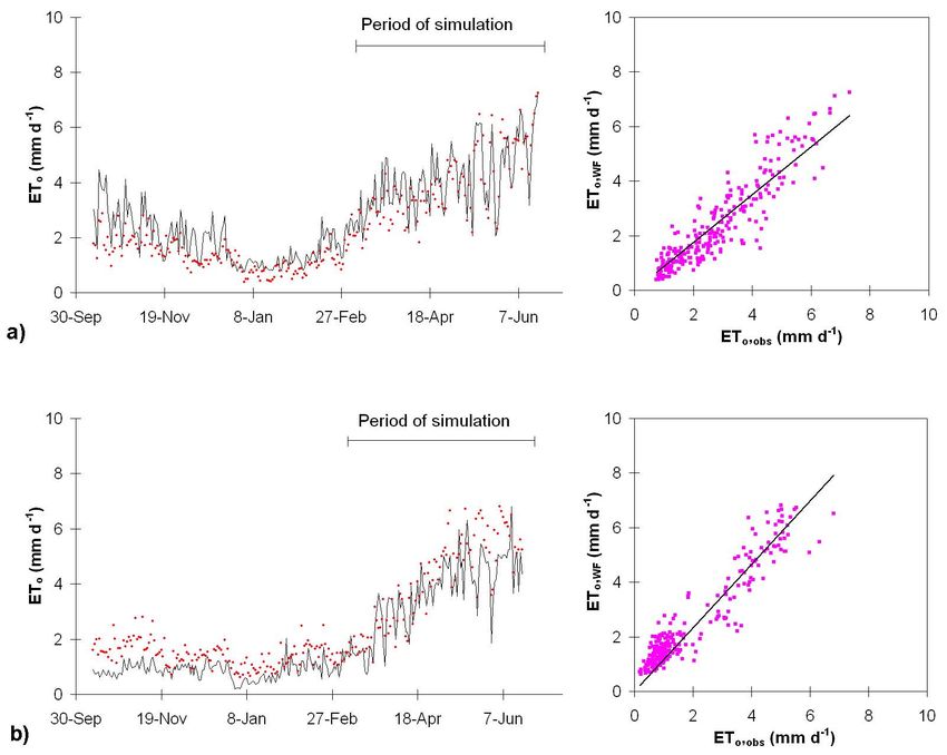
J. B. Cai et al.: Water balance with weather forecasts                                                                       1047

   The daily wind speed (uz ) at height z is obtained from
the weather forecast messages of wind grade following the
standards of meteorological observation (CMA, 2003) using
a conversion table reported by Cai et al. (2007). The wind
speed at 2 m height (u2 ) is then obtained from uz through the
following equation:

                4.87
u2 = uz                                                    (4)
          ln (67.8z−5.42)

where u2 is the wind speed at 2 m height (m s−1 ), uz is the
measured wind speed at height z (m s−1 ), and z is the height
of wind measurements above the ground surface (m).

2.2   Field experiments and data collection

Field experiments with winter wheat (Triticum aestivum L.)
were carried out at the Irrigation Experiment Station of the
China Institute of Water Resources and Hydropower Re-
search (IWHR) at Daxing, south of Beijing (39◦ 370 N lati-
tude, 116◦ 260 E longitude and 40.1 m a.s.l. elevation). Wheat
is the main irrigated crop in the region. The climate in
the experimental site is semiarid to sub-humid, with cold
and dry winter and hot and humid summer, when monsoon
rains occur. Further information on the climate in the North
China Plain is provided by Wang et al. (2008). An auto-
matic weather station is installed in the experimental station,   Fig. 1. Average weather characteristics of the winter wheat crop
which provides for measurements of air temperature, relative      season at Daxing, 1995–2005: (a) monthly temperature (2) and
humidity, global and net radiation, wind speed at 2 m height,     relative humidity (N); (b) monthly precipitation () and reference
soil temperature at various depths, and precipitation. The av-    evapotranspiration, ETo (•).
erage values of main climatic variables for the period 1995–
2005 are presented in Fig. 1 for the winter wheat growing
season. The behaviour of main climate variables in the area       demonstrations in farmers fields aimed at reducing the de-
is reported by Pereira et al. (1998, 2003a).                      mand and controlling groundwater use (Pereira et al., 1998,
   Soils in this area of the North China Plain are silty soils    2003a). The experimental area is part of the network of ex-
formed by deposits of the loess formations. It was observed       perimentation developed to improve soil and water manage-
that the soil hydraulic properties relevant for water balance     ment, and regular observations of the groundwater table are
studies vary little in the area (Ding, 1998; Liu and Pereira,     performed. Information to farmers is provided by local ex-
2003; Pereira et al., 1998, 2003a; Xu and Mermoud, 2003).         tension officers. Observations at Daxing have shown that the
The soil in the experimental area is a silt loam, with aver-      groundwater table is there at a depth near 18 m; therefore,
age field capacity (θFC ) and wilting point (θWP ) of 0.334 and   capillary rise from the groundwater was not considered in
0.128 m3 m−3 in the crop root zone (1 m depth). θFC and θWP       the soil water balance calculations.
were measured in laboratory as the soil water content at re-         The experiments were developed during two winter wheat
spectively 33 and 1500 kPa suction pressure. The main soil        growing seasons, 2005–2006 and 2006–2007. Wheat is the
hydraulic properties are presented in Table 1. Soil salinity      main irrigated crop in the area; a few horticultural crops are
is not a problem in the area because the monsoon rains pro-       also practiced but wheat is the one having by far the highest
vide for natural leaching; however, the application of gypsum     demand for water. Summer crops are irrigated only when
may be considered among the soil management practices de-         the monsoon rains are scarce. The experiments were de-
sirable for the area (Ding, 1998; Pereira et al., 1998, 2003a).   signed for both the evaluation of the performance of using
   The groundwater in North China Plain is over-exploited,        WF data to compute ETo and for agronomic assessment of
including for irrigation purposes, causing large water table      irrigation scheduling and fertilization practices but results of
depletion when a succession of dry years occurs (e.g. Cai et      agronomic nature are not analysed in this paper. The experi-
al., 1996; Randin et al., 1999; Zhao et al., 2004; Nakayama       ments were based upon results of former studies in the North
et al., 2006). This problem led to develop studies in the         China Plain aimed at developing water saving practices (e.g.,
area aimed at developing appropriate irrigation practices and     Liu et al., 1998, 2004; Pereira et al., 1998, 2003a). Water

www.hydrol-earth-syst-sci.net/13/1045/2009/                                      Hydrol. Earth Syst. Sci., 13, 1045–1059, 2009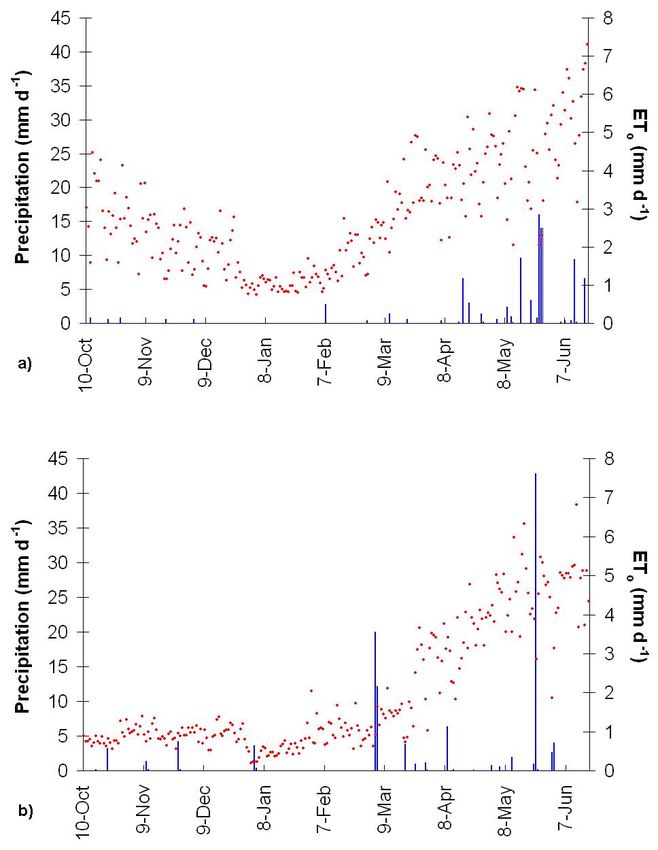
1048                                                                                J. B. Cai et al.: Water balance with weather forecasts

Table 1. Main soil hydraulic properties for water balance purposes in Daxing experimental station.

                       Layer     Depth     Bulk density     Saturated water content      Field capacity   Wilting point
                                 (cm)       (g cm−3 )              (m3 m−3 )               (m3 m−3 )       (m3 m−3 )
                         1       0∼10           1.30                   0.46                  0.32             0.09
                         2      10∼20           1.46                   0.46                  0.34             0.13
                         3      20∼40           1.48                   0.47                  0.35             0.10
                         4      40∼60           1.43                   0.45                  0.33             0.11
                         5      60∼100          1.39                   0.44                  0.31             0.16

                                                                             The experiments were performed using a randomized
                                                                          block design with three or more plots per treatment. Every
                                                                          plot was 5.5×5.5 m in a N-S row direction. There were four
                                                                          irrigation treatments for 2005–2006 (W1 to W4) and five for
                                                                          2006–2007 (T1 to T5). All irrigation treatments were per-
                                                                          formed with basin irrigation and conventional tillage. All
                                                                          treatments received a winter irrigation that refilled the soil
                                                                          reservoir to field capacity. The irrigation treatments were
                                                                          different in both years due to different agronomic objec-
                                                                          tives including the application of a light irrigation by early
                                                                          spring aimed at fertigation in the second year. The appli-
                                                                          cation depths are given in Table 2 and the criteria for the
                                                                          irrigation timings are described as follows:

                                                                          W1 – rain fed from the winter to harvesting;

                                                                          W2 – mild water stress, with a soil water threshold equal to
                                                                             60% of θFC ;

                                                                          W3 – mild water stress with a soil water threshold equal to
                                                                             60% of θFC , with smaller water depths than W2;

                                                                          W4 – irrigation timings and depths as recommended by the
                                                                             farmer’ adviser for water saving;

                                                                              T1 – no water stress with a soil water threshold equal to
                                                                                 80% of θFC ;

                                                                              T2 – no water stress with a soil water threshold equal to
Fig. 2. Daily ETo (•) and precipitation (|) during the wheat experi-
ments: (a) 2005–2006; and (b) 2006–2007.                                         70% of θFC ;

                                                                              T3 – mild water stress with a soil water threshold equal to
savings result from combining improved irrigation schedul-                       60% of θFC ;
ing with the amelioration of the basin irrigation systems (Fer-
                                                                              T4 – mild water stress at the late stages of the crop, when
nando et al., 1998; Liu et al., 2000, 2004; Liu and Pereira,
                                                                                 the soil water threshold was equal to 60% of θFC ;
2003). Studies on basin irrigation practices (Bai et al., 2005)
were developed in parallel with this research aiming at fur-                  T5 – irrigation timings and depths as recommended by the
ther developments in water saving irrigation.                                    farmer’ adviser for water saving.
   The daily ETo and precipitation for both seasons are
shown in Fig. 2. The wheat crop season developed from                        The soil water content was measured every 4 days in each
10 October to 18 June for both years. The total precipitation             plot with two replicates using a time-domain reflectometry
was 99.6 mm for 2005–2006 and 112.6 mm for 2006–2007;                     (TDR) system TRIME® -T3/IPH from 0.2 to 1.2 m depth
in this season there were less rainfall events than for the pre-          with observations every 0.2 m. The TDR measuring accu-
vious one. There were no noticeable differences in season                 racy is 2%. For the surface layer, soil samples were taken to
ETo .                                                                     be dried in the oven. Crop heights were observed every ten

Hydrol. Earth Syst. Sci., 13, 1045–1059, 2009                                              www.hydrol-earth-syst-sci.net/13/1045/2009/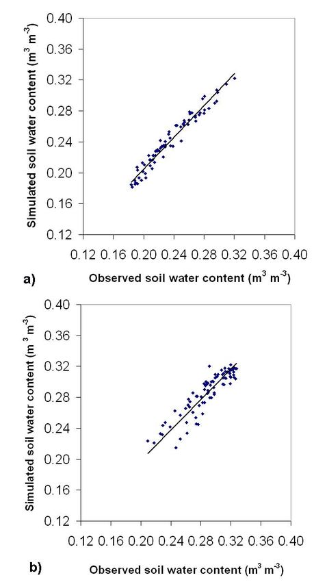
J. B. Cai et al.: Water balance with weather forecasts                                                                            1049

Table 2. Irrigation treatments: applied water depths and dates.

  Crop season     Treatment     Initial stage (winter irrigation)   Development stage         Mid-season Stage           Late stage
   2005–2006         W1                 90 mm (20/11)
                     W2                 90 mm (20/11)               90 mm (05/04)               80 mm (12/5)
                     W3                 90 mm (20/11)               65 mm (05/04)              80 mm (05/05)
                     W4                 90 mm (20/11)               115 mm (05/04)            115 mm (12/05)
   2006–2007         T1                 90 mm (18/11)               30 mm (06/04)∗      60 mm (21/04), 63 mm (07/05)   67 mm (04/06)
                     T2                 90 mm (18/11)               30 mm (06/04)∗      97 mm (30/04), 84 mm (14/05)
                     T3                 90 mm (18/11)               30 mm (06/04)∗            102 mm (07/05)
                     T4                 90 mm (18/11)               30 mm (06/04)∗             65 mm (26/04)           86 mm (04/06)
                     T5                 90 mm (18/11)               30 mm (06/04)∗             96 mm (07/05)           70 mm (04/06)

Note: Numbers in brackets refer to the day and month of the irrigation event.
∗ Fertilizers were applied with this irrigation event.

days. Yields and yield components were observed at harvest-               Mediterranean region (Oweis et al., 2003; Zairi et al., 2003),
ing. Field measurements were performed only after the soil                North China (Liu et al., 1998, 2006; Pereira et al., 2007),
defrosts, when the crop has started growing by the end of the             South America (Victoria et al., 2005), Central Asia (Fortes
winter. The water was conveyed to the fields by a PVC pipe                et al., 2005; Cholpankulov et al., 2008) and Europe (Popova
from the well pump where discharge was measured with a                    et al., 2006a; Cancela et al., 2006). The model performs the
flowmeter. Water applications were controlled by an auto-                 irrigation scheduling simulations according to the following
mated low pressure valve.                                                 user-defined options:
   Weather data were collected every 30 min and integrated
to the hour. These hourly values were used to compute                       – to define an irrigation scheduling to maximize crop
the ETo,obs adopting the procedures described by Allen et                     yields, i.e. without crop water stress;
al. (1998, 2006). The ETo,WF was computed daily from the
weather forecast messages available from the Beijing Daily                  – to generate an irrigation scheduling using selected irri-
Newspaper acceded through the web. This allowed adopting                      gation thresholds, including for an allowed water stress,
automatic digital processing of those messages to compute                     and responding to water availability restrictions im-
ETo,WF .                                                                      posed at given time periods;

2.3   Simulation of the soil water balance                                  – to evaluate yield and water use impacts of a given irri-
                                                                              gation schedule;
The ISAREG model (Teixeira and Pereira, 1992) was used
                                                                            – to test the model performance against observed soil wa-
to simulate the soil water balance for all treatments using
                                                                              ter data and using actual irrigation dates and depths,
both ETo,obs and ETo,WF as inputs, which allowed assessing
                                                                              which is the option used for calibration and validation
the accuracy of ETo,WF as input for modelling. ISAREG is
                                                                              in this study;
an irrigation scheduling simulation model that performs the
soil water balance at the field scale. The model is described
                                                                            – to execute the water balance without irrigation; and
in detail by Teixeira and Pereira (1992), Liu et al. (1998)
and Pereira et al. (2003b), the latter referring to the Windows             – to compute the net crop irrigation requirements, and
version of the model. The water balance model ISAREG was                      performing the respective analysis of frequencies when
selected after comparing its results with those from the wa-                  a weather data series is considered.
ter flux model WAVE (Vanclooster et al., 1995) for irrigation
scheduling purposes and considering that data requirements                The model input data for a daily time step computation in-
for water balance simulations are much less than for flux sim-            cludes:
ulations (Pereira et al., 1998). However, because WAVE ac-
curately computed capillary rise and percolation, it was used               1. Meteorological data concerning precipitation, P
to support developing a set of parametric equations for esti-                  (mm d−1 ) and reference evapotranspiration, ETo
mating these variables with ISAREG (Liu et al., 2006).                         (mm d−1 ), or daily weather data to compute ETo with
   The water balance is performed for various time-step com-                   the FAO-PM methodology, including alternative com-
putations depending on weather data availability. The model                    putation methods for missing climate data as for this
is used for a variety of crops and environments, e.g. in the                   study (Allen et al., 1998; Popova et al., 2006b);

www.hydrol-earth-syst-sci.net/13/1045/2009/                                             Hydrol. Earth Syst. Sci., 13, 1045–1059, 2009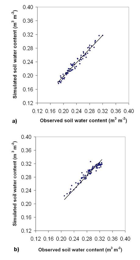
1050                                                                      J. B. Cai et al.: Water balance with weather forecasts

 2. Soil data for a multi-layer soil relative to each layer,      where Kc is the crop coefficient and ETo is the reference
    the respective depth d (m); the soil water content            evapotranspiration (mm d−1 ). Then, between two irrigation
    at field capacity θFC (m3 m−3 ) and the wilting point         events, R varies linearly with the time t as
    θWP (m3 m−3 ), and the initial soil water content θin
                                                                  Rt = Ro + (Win − ETm ) t                                     (8)
    (m3 m−3 ) in the soil profile; additional data not used in
    this study refer to the parameters for the equations rel-     where Ro is the initial value of R in the considered time pe-
    ative to groundwater contribution, percolation; and soil      riod (mm), and Win is the water input to the root zone storage
    salinity.                                                     (mm) due to precipitation and capillary rise. A daily time
                                                                  step computation is used.
 3. Crop data referring to dates of crop development stages,         When R
J. B. Cai et al.: Water balance with weather forecasts 1051
m
P
Oi × Pi Table 3. Statistical indicators comparing ETo computations us-
i=1 ing fully observed data sets (ETo,obs ) and weather forecasted data
b= m (12)
P
Oi2 (ETo,WF ) for two wheat crop seasons.
i=1
– Coefficient of determination, R 2 : b R2 RMSE RE EF d
2 (mm d−1 )
Pm
Oi − O P i − P 2005–2006 0.878 0.834 0.764 0.272 0.746 0.939
2 i=1 2006–2007 1.163 0.850 0.771 0.389 0.767 0.945
R = 0.5 m
(13)
m 2 0.5
P Oi − O 2
P
Pi − P
i=1 i=1
– Root Mean Square Error, RMSE:
underestimation of the climatic parameters of the Penman-
m
P 0.5 Monteith reference evapotranspiration and respective results.
(Pi −Oi )2 Figure 3 compares the daily values of ETo computed with ob-
i=1
RMSE= (14) served weather data (ETo,obs ) and with WF data (ETo,WF ).
m
Considering the regression forced to the origin when com-
paring both sets of daily ETo values it may be observed that
– Relative Error, RE: ETo,WF is underestimated in relation to ETo,obs for the wheat
crop season 2005–2006, while it is overestimated for 2006–
RMSE 2007 The regression coefficients are respectively 0.88 and
RE= (15)
O 1.16, and the corresponding R 2 values are high, respectively
– Modelling efficiency, EF: 0.83 and 0.85. Results in Table 3 show that the RMSE val-
ues are relatively small: 0.76 and 0.77 mm d−1 for the 2005–
m 2006 and 2006–2007 crop seasons, respectively. These er-
(Oi −Pi )2
P
i=1
rors are similar to those observed earlier in North China
EF=1.0− m (16) when estimating ETo from maximum and minimum temper-
P 2
Oi −O ature (Pereira et al., 2003a), and those observed by Popova
i=1 et al. (2006b) for South Bulgaria when performing the same
– The Willmott index of agreement, d: type of ETo estimation. However, those errors are near to
the upper range of those referred by Cai et al. (2007) for
m
P
(Oi − Pi )2 estimating ETo from WF at eight locations in China. The
i=1 relative errors are 0.27 and 0.39 for the two seasons consid-
d =1− m (17) ered (Table 3), which are larger than those computed for the
P 2
Pi − O + Oi − O eight locations. These RE values decrease to 0.18 and 0.25
i=1
when only the data relative to the period of simulation are
where the m is the number of observations, Oi and Pi are considered, i.e., after crop reviving until harvesting, because
respectively the i-th observed and predicted data; O is the the ETo values are then larger than those for the autumn and
average value for Oi with i=1, 2,. . . , m, P is the average of winter period, thus impacts of inaccuracy in weather fore-
the data arrays of Pi . The values of EF and d vary from 0 to casting result then relatively less important. The values for
1.0 according to the quality of model fitting and are desirably the index d are high (0.94 and 0.95) and the modelling effi-
close to 1.0. The estimation error indicators RE and RMSE ciency EF is also high, with values 0.75 and 0.77 respectively
are hoped to be as small as possible. The coefficient b may be for 2005–2006 and 2006–2007.
larger or smaller than 1.0 when there is respectively overes- The smaller accuracy of estimation relatively to the former
timation or underestimation of the target variable. When R 2 study performed for synoptic stations (Cai et al., 2007) was
is close to 1.0 the variance of the estimation errors is small. expected. The synoptic stations are explored by the China
Meteorological Administration (CMA) and provide informa-
3 Results and discussion tion on conditions of the atmosphere or weather as they ex-
ist simultaneously over a broad area and where observations
3.1 Comparing ETo estimates obtained from observed are made at periodic times (usually at 3-hourly and 6-hourly
and forecast messages weather data intervals specified by the World Meteorological Organiza-
tion), These observations are used to provide information
As analysed by Cai et al. (2007), the weather forecasted data for the global and regional circulation models used for the
do not exactly match those observed and lead to over- or weather forecasts at the same locations. Therefore, when
www.hydrol-earth-syst-sci.net/13/1045/2009/ Hydrol. Earth Syst. Sci., 13, 1045–1059, 20091052 J. B. Cai et al.: Water balance with weather forecasts
Fig. 3. Comparison of the ETo values computed from observed and weather forecast messages data for the wheat crop season (a) for 2005–
2006 and (b) for 2006–2007. On the left, the daily course of ETo,obs , (—) and ETo,WF (•) from planting (October) to harvesting (June); on
the right, the respective regression forced to the origin.
extrapolating these forecasts for non-synoptic weather sta- Table 4. Wheat crop coefficients Kc and depletion fractions for
tions, as in this study, it is expected that the forecasts will no stress p obtained from model calibration in the crop season of
over- or under-predict the weather variables relatively to ob- 2005–2006.
servations at the same locations. The fact that in the first
season there was an over-prediction of ETo and in the sec-
ond ETo was under-predicted may indicate that there is not a Crop growth stages Dates1 Kc p
systematic error of prediction.
Crop development (01/03∼20/04) 0.40–1.00 0.60–0.50
Overall, the results obtained indicate that estimating daily
Mid-season (21/04∼31/05) 1.00 0.50
ETo from weather forecast messages is feasible for locations End season (01/06∼18/06) 1.00–0.30 0.50–0.60
out of the network of CMA synoptic weather stations de-
spite the forecasting accuracy is smaller than for synoptic 1 Numbers in brackets refer to the day and month respectively.
stations. This fact justifies the need to assess the impacts of
using ETo,WF estimates instead of ETo,obs when performing
the soil water balance for irrigation scheduling, whose re- 2005–2006 were used for the calibration and those of 2006–
sults are analysed below. Results indicate the need to further 2007 were used for validation. The calibration led to appro-
study the spatial variation of ETo,WF estimates when using priate values for the crop coefficients Kc and the depletion
them for providing real-time irrigation scheduling advising fractions p, which are given in Table 4. The calibration was
at project, basin or regional level. performed iteratively until the simulated soil water content
matches the observed one. Initial values for the crop param-
3.2 Model calibration and validation eters were those tabled by Allen et al. (1998) after being cor-
rected for climate as suggested by these authors. The simu-
The calibration and validation of the model ISAREG was lations concern the period after soil defrost or crop reviving,
performed using ETo,obs data. Irrigation treatments data for i.e. the crop development, mid season and late season stages.
Hydrol. Earth Syst. Sci., 13, 1045–1059, 2009 www.hydrol-earth-syst-sci.net/13/1045/2009/J. B. Cai et al.: Water balance with weather forecasts 1053
Table 5. Statistical indicators for model goodness of fitting when Table 6. Statistical indicators for model goodness of fitting when
comparing the soil water content observed and predicted by the comparing the soil water content observed and predicted by the
model for the treatments used for calibration and validation. model f when ETo was estimated from weather forecast messages
(ETo,WF ).
b R2 RMSE RE EF d
(m3 m−3 ) b R2 RMSE RE EF d
Calibration (2005–2006) (m3 m−3 )
W1 0.98 0.85 0.007 0.035 0.69 0.94 2005–2006
W2 0.98 0.92 0.008 0.035 0.89 0.97 W1 1.01 0.78 0.007 0.037 0.64 0.93
W3 0.99 0.89 0.006 0.027 0.88 0.97 W2 1.02 0.92 0.010 0.039 0.87 0.97
W4 1.02 0.96 0.006 0.024 0.97 0.99 W3 1.04 0.83 0.012 0.052 0.55 0.89
All treatments 0.99 0.97 0.007 0.030 0.96 0.99 W4 1.00 0.97 0.009 0.035 0.93 0.98
Validation (2006–2007) All treatments 1.03 0.95 0.010 0.041 0.92 0.98
T1 1.02 0.75 0.009 0.030 0.77 0.93 2006–2007
T2 1.02 0.62 0.003 0.010 0.66 0.90 T1 0.98 0.74 0.012 0.041 0.57 0.90
T3 1.00 0.88 0.008 0.028 0.92 0.98 T2 1.00 0.78 0.009 0.031 0.78 0.94
T4 1.02 0.93 0.010 0.037 0.92 0.98 T3 0.96 0.84 0.016 0.057 0.69 0.93
T5 1.01 0.87 0.010 0.034 0.89 0.97 T4 0.99 0.93 0.010 0.037 0.92 0.98
All treatments 1.01 0.92 0.010 0.034 0.88 0.97 T5 0.98 0.80 0.013 0.046 0.80 0.94
All treatments 0.99 0.82 0.012 0.043 0.81 0.95
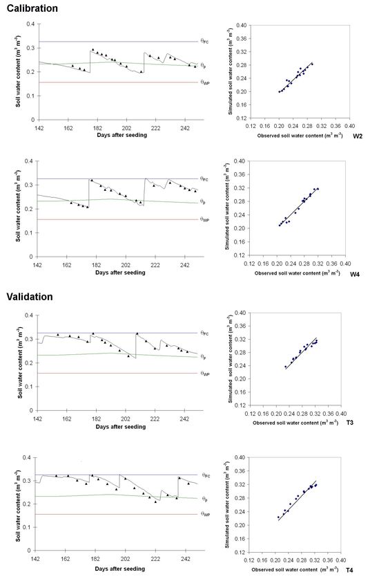
Results comparing the soil water content observed and
simulated for the calibration are shown in Fig. 4 for two treat-
ments (W2 and W4) and in Fig. 5a for all treatments W1 to Considering both the calibration and validation results, it
W4. Moreover, because a rainfed treatment (W1) is included, was verified that errors are smaller than those observed in
the calibration was performed for the full range of soil wa- former studies (Liu et al., 1998). It was also observed that
ter content values expected in the practice. The statistical the irrigation schedules adopted for water saving (W4 and
indicators for the goodness of model fitting are presented in T5) effectively respond to this objective and provided for wa-
Table 5. For the four treatments, the coefficient of regression ter productivities among the highest in both years. It can be
range 0.98 to 1.02, thus very close to the target 1.0 value. concluded that the model performed very well to predict the
The determination coefficients are quite high, ranging 0.85 soil water content of the wheat crop during the development,
to 0.96. The estimation errors are small, with RMSE vary- mid-season and end-season crop stages.
ing in a very short range (0.006 to 0.008 m3 m−3 ); RE values
are also small, ranging from 0.024 to 0.035. The values for 3.3 Accuracy of model predictions when ETo is esti-
d and EF show that model fitting is good, with d ranging mated from weather forecast messages
0.94 to 0.99 and EF varying from 0.69 to 0.97. These re-
sults show that the simulated soil water content matches well All treatments were simulated with the model using the cal-
with the observed values, i.e., the model accurately simulates ibrated crop parameters given in Table 4 and adopting as
the soil water balance of the wheat crop when the calibrated model input the WF estimated ETo,WF instead of ETo,obs .
parameters are used. The initial soil water content values used for these simula-
The results for the validation with field data from the treat- tions are the same as for the calibration and validation. Re-
ments of 2006–2007 are similar to those obtained for the cal- sults for the goodness of model predictions of the soil water
ibration. Figure 4 shows the observed and simulated soil content are given in Table 6. Selected simulation results for
water for treatments T3 and T4, and in Fig. 5b results are the treatments W2 and W4 in 2006, and T3 and T4 in 2007
shown for all treatments T1 to T5. The statistical indicators are shown in Fig. 6. Results for all treatments and both crop
for goodness of model predictions are presented in Table 5. seasons are presented in Fig. 7. As noted above, since treat-
The b values are just slightly higher than those for the cal- ments include rainfed and no water stress ones, the soil water
ibration, and R 2 range from 0.62 to 0.93. The estimations content observations cover the full range of values expected
errors are also slightly higher than for the calibration, with in the practice.
RMSE=0.010 m3 m−3 and RE=0.034 when all treatments are The coefficients of regression are close to 1.0 (Table 6),
considered. The d and EF indices are consequently slightly ranging 1.0 to 1.04 for 2006 and from 0.96 to 1.0 in 2007, i.e.,
smaller than those for the calibration, with d ranging 0.90 to there is a slight overestimation of the soil water content in
0.98 and EF ranging 0.66 to 0.92. These results indicate that 2006 when ETo , was underestimated, and underestimation in
the parameters obtained at calibration are appropriate for the 2007 when ETo, was overestimated. However, the under- and
model simulations aimed at irrigation scheduling. over-estimation resulting for the prediction of the soil water
www.hydrol-earth-syst-sci.net/13/1045/2009/ Hydrol. Earth Syst. Sci., 13, 1045–1059, 20091054 J. B. Cai et al.: Water balance with weather forecasts Fig. 4. Comparing the soil water content observed and predicted by the model for two calibration treatments (W2 and W4) and two validation treatments (T3 and T4). On the left: the daily course of the soil water; on the right, the respective regressions forced to the origin. The lines of θFC , θp and θWP refer to the soil water content at field capacity, at the depletion fraction for no stress and at the wilting point, respectively. Hydrol. Earth Syst. Sci., 13, 1045–1059, 2009 www.hydrol-earth-syst-sci.net/13/1045/2009/
J. B. Cai et al.: Water balance with weather forecasts                                                                     1055

                                                                   use as model input the reference evapotranspiration estimates
                                                                   ETo,WF with appropriate accuracy for irrigation scheduling
                                                                   purposes. It is then possible to run a model in real time with
                                                                   daily inputs of ETo,WF and actual observations of precipita-
                                                                   tion. Further research is required to combine a spatialized
                                                                   ETo,WF estimation as referred above with the operation of
                                                                   the irrigation scheduling model with a spatial GIS database
                                                                   as formerly tested (Fortes et al., 2005).

                                                                   4   Conclusions

                                                                   This study has shown that the reference evapotranspiration
                                                                   can be estimated from daily weather forecast messages using
                                                                   the FAO Penman Monteith equation in a non-synoptic loca-
                                                                   tion, however with less accuracy then for synoptic stations.
                                                                   With this approach, the global radiation is estimated from the
                                                                   difference between the forecasted maximum and minimum
                                                                   temperatures, the actual vapour pressure is estimated from
                                                                   the forecasted minimum temperature and the wind speed is
                                                                   obtained from converting the common wind scales used by
                                                                   the China Meteorological Administration into wind speed.
                                                                   The estimated ETo shows a RMSE of 0.77 mm d−1 and the
                                                                   indicators EF and d for the goodness of fitting average 0.75
                                                                   and 0.94, respectively. These indicators show that using daily
                                                                   weather forecasts produces estimates for ETo comparable
                                                                   with those computed with observed weather data, particu-
                                                                   larly when some weather variables are not observed. These
                                                                   results indicate that daily forecast messages may be used
                                                                   for ETo computations for non-synoptic locations which pro-
                                                                   vide for adopting ETo,WF .for real time irrigation schedul-
                                                                   ing models. However, further studies on the spatial vari-
Fig. 5. Linear regression forced to the origin comparing the ob-
                                                                   ation of ETo,WF estimates are required to better assess the
served and model predicted soil water content for all treatments
                                                                   conditions to use them for real-time irrigation scheduling at
used for calibration (a) and validation (b).
                                                                   project, basin or regional level.
                                                                      To assess the impacts of using ETo,WF estimates instead
                                                                   of ETo,obs when modelling the soil water balance, the model
content are much smaller than those for ETo,WF . It results        ISAREG was first calibrated and validated for several winter
that differences in b values are very small when the ETo,obs       wheat treatments and using ETo,obs as input data for the crop
or ETo,WF data sets are used. The determination coefficients       seasons of 2005–2006 and 2006–2007. Simulations were
range 0.78 to 0.97 for the first year and 0.74 to 0.93 for the     performed for the period after soil defrost and crop reviv-
second, and are slightly smaller than those obtained for the       ing after the winter, thus during the development, mid-season
calibration and validation of the model.                           and end-season crop stages. The respective results show that
   When computations are performed with ETo,WF the es-             the simulated soil water content matches well with the ob-
timation errors RMSE and RE are small but slightly larger          served values, i.e., the model accurately simulates the soil
than those using ETo,obs . Considering all treatments, RMSE        water balance of the wheat crop when the calibrated param-
averages 0.010 and 0.012 m3 m−3 for respectively 2006 and          eters are used.
2007, while RE is 0.041 and 0.043 for the same years (Ta-             The results of the simulations for both crop seasons and
ble 6). These good results are confirmed by the d and EF           the same irrigation treatments using ETo,WF have also shown
indices, whose values range respectively from 0.89 to 0.98         that the simulated soil water content matches well with the
and from 0.55 to 0.93 when considering both years. Results         observed values. However, the over- or under estimation
in Fig. 7 confirm the goodness of fitting for all treatments       of ETo produces, respectively, a small under- and over-
simulated.                                                         estimation of the simulated soil water content. In the present
   These results indicate that when the soil water balance is      study, the RMSE values ranged from 0.007 to 0.016 m3 m−3 ,
performed with a properly calibrated model it is possible to       which indicates a very good modelling accuracy. Other

www.hydrol-earth-syst-sci.net/13/1045/2009/                                      Hydrol. Earth Syst. Sci., 13, 1045–1059, 2009
1056 J. B. Cai et al.: Water balance with weather forecasts Fig. 6. Comparing the soil water content observed and predicted by the model when ETo was estimated from weather forecast messages (ETo,WF ) for: (a) two treatments in 2005–2006 (W2 and W4); and (b) two other treatments in 2006–2007 (T3 and T4). On the left: the daily course of the soil water; on the right, the respective regressions forced to the origin. The lines of θFC , θp and θWP refer to the soil water content at field capacity, at the depletion fraction for no stress and at the wilting point, respectively. Hydrol. Earth Syst. Sci., 13, 1045–1059, 2009 www.hydrol-earth-syst-sci.net/13/1045/2009/
J. B. Cai et al.: Water balance with weather forecasts                                                                               1057

                                                                    References

                                                                    Allen, R. G., Pereira, L. S., Raes, D., and Smith, M.: Crop Evapo-
                                                                      transpiration: Guidelines for computing crop requirements. FAO,
                                                                      Irrigation and Drainage Paper No. 56, FAO, Rome, Italy, 300 pp.,
                                                                      1998.
                                                                    Allen, R. G., Pruitt, W. O., Wright, J. L., Howell, T. A., Ventura,
                                                                      F., Snyder, R., Itenfisu, D., Steduto, P., Berengena, J., Baselga,
                                                                      J., Smith, M., Pereira, L. S., Raes, D., Perrier, A., Alves, I.,
                                                                      Walter, I., and Elliott, R.: A recommendation on standardized
                                                                      surface resistance for hourly calculation of reference ETo by the
                                                                      FAO56 Penman-Monteith method, Agric. Water Manage., 81, 1–
                                                                      22, 2006.
                                                                    Angström, A.: Solar and terrestrial radiation, Q. J. Roy. Meteor.
                                                                      Soc., 50, 121–125, 1924.
                                                                    Bai, M. J., Xu, D., Li, Y. N., and Li, J. S.: Evaluation of spatial and
                                                                      temporal variability of infiltration on a surface irrigation field, J.
                                                                      Soil Water Conserv,, 19(5), 120–123, 2005 (in Chinese).
                                                                    Cabelguenne, M., Debaeke, Ph., Puech, J., and Bose, N.: Real
                                                                      time irrigation management using the EPIC-PHASE model and
                                                                      weather forecasts, Agric. Water Manage., 32, 227–238, 1997.
                                                                    Cai, L. G., Qian, Y., and Xu, D.: Sustaining irrigated agriculture
                                                                      in China, in: Sustainability of Irrigated Agriculture, edited by:
                                                                      Pereira, L. S., Feddes, R. A., Gilley, J. R., and Lesaffre, B.,
                                                                      NATO ASI Series, Kluwer, Dordrecht, 581–587, 1996.
                                                                    Cai, J. B., Liu, Y., Lei, T., and Pereira, L. S.: Estimating reference
                                                                      evapotranspiration with the FAO Penman-Monteith equation us-
                                                                      ing daily weather forecast messages, Agric. For. Meteo., 145(1–
                                                                      2), 22–35, 2007.
                                                                    Calera Belmonte, A., Jochum, A. M., Cuesta Carcia, A., Montoro
                                                                      Rodriguez, A., and López Fuster, P.: Irrigation management from
                                                                      space: Towards user-friendly products, Irrig. Drain. Syst., 19,
                                                                      337–354, 2005.
                                                                    Cancela, J. J., Cuesta, T. S., Neira, X. X., and Pereira, L. S.: Mod-
Fig. 7. Linear regression forced to the origin comparing the ob-      elling for improved irrigation water management in a temperate
served and model predicted soil water content when ETo was com-       region of Northern Spain, Biosyst. Eng., 94(1), 151–163, 2006.
puted from weather forecast messages (ETo,WF ) for all treatments   Chavez, J., Neale, C. M. U., Prueger, J. H., and Kustas, W. P.:
of 2005–2006 (a) and 2006–2007 (b).                                   Daily evapotranspiration estimates from extrapolating instanta-
                                                                      neous airborne remote sensing ET values, Irrig. Sci., 27, 67–81,
model fitting indicators confirm these results, with EF rang-         2008.
ing 0.55 to 0.92 and d ranging 0.89 to 0.98. It can be con-         Cholpankulov, E. D., Inchenkova, O. P., Paredes, P., and Pereira, L.
                                                                      S.: Cotton irrigation scheduling in Central Asia: Model calibra-
cluded that when the soil water balance is performed with a
                                                                      tion and validation with consideration of groundwater contribu-
properly calibrated model it is appropriate to use as model
                                                                      tion, Irrig. Drain., 57, 516–532, 2008.
input the reference evapotranspiration estimated from daily         CMA: Surface Meteorological Observation Criterion, China Mete-
weather forecast messages. However, further research on the           orological Administration, Beijing, 2003 (in Chinese).
spatial variation of ETo,WF estimates and of their impacts          Consoli, S., D’Urso, G., and Toscano, A.: Remote sensing to es-
on model predictions of the soil water content is required            timate ET-fluxes and the performance of an irrigation district in
and is being developed to better assess the conditions for us-        southern Italy, Agric. Water Manage., 81, 295–314, 2006.
ing those ETo estimates for real-time irrigation scheduling at      Courault, D., Seguin, B., and Olioso, A.: Review on estimation of
project, basin or regional level.                                     evapotranspiration from remote sensing data: From empirical to
                                                                      numerical modeling approaches, Irrig. Drain. Syst., 19, 223–249,
Acknowledgements. This research was supported by the Projects         2005.
of Development Plan of the State Key Fundamental Research           Ding, K. L. An investigation into the effects of soil management on
(No. 2006CB403405) and by the National 863 Plans Project              soil properties and crop growth in the Huang-Huai-Hai Plain in
No. 2006AA100208-4. The collaborative Sino-Portuguese project         North China. PhD dissertation, Silsoe College, Cranfield Univer-
on “Water Saving Irrigation: Technologies and Management” is          sity, 1998.
also acknowledged.                                                  Donatelli, M., Bellocchi, G., and Fontana, F.: RadEst3.00: software
                                                                      to estimate daily radiation data from commonly available meteo-
Edited by: G. Blöschl                                                rological variables, Eur. J. Agron., 18, 363–367, 2003.

www.hydrol-earth-syst-sci.net/13/1045/2009/                                         Hydrol. Earth Syst. Sci., 13, 1045–1059, 2009
1058 J. B. Cai et al.: Water balance with weather forecasts Fernando, R. M., Pereira, L. S., Liu, Y., Li, Y. N., and Cai, L. coupled hydrology and agricultural models, Hydrol. Processes, G.: Reduced demand irrigation scheduling under constraint of 20, 3441–3466, 2006. the irrigation method, in: Water and the Environment: Innova- Oweis, T., Rodrigues, P. N., and Pereira, L. S.: Simulation of sup- tion Issues in Irrigation and Drainage (1st Inter-Regional Conf. plemental irrigation strategies for wheat in Near East to cope Environment-Water, Lisbon), edited by: Pereira, L. S. and Gow- with water scarcity, in: Tools for Drought Mitigation in Mediter- ing, J. W., E& FN Spon, London, 407–414, 1998. ranean Regions, edited by: Rossi, G., Cancelliere, A., Pereira, L. Fortes, P. S., Platonov, A. E., and Pereira, L. S.: GISAREG – A S., Oweis, T., Shatanawi, M., and Zairi, A., Kluwer, Dordrecht, GIS based irrigation scheduling simulation model to support im- 259–272, 2003. proved water use, Agric. Water Manage., 77, 159–179, 2005. Pereira, L. S., Musy, A., Liang, R. J., and Hann, M. (Eds.): Water Garatuza-Payan, J. and Watts, C. J.: The use of remote sensing for and Soil Management for Sustainable Agriculture in the North estimating ET of irrigated wheat and cotton in Northwest Mex- China Plain, ISA, Lisbon, 405 pp., 1998. ico, Irrig. Drain. Syst., 19, 301–320, 2005. Pereira, L. S., Cai, L. G., and Hann, M. J.: Farm water and soil Gowda, P. H., Chavez, J. L., Colaizzi, P. D., Evett, S. R., Howell, management for improved water use in the North China Plain, T. A., and Tolk, J. A.: ET mapping for agricultural water man- Irrig. Drain., 52(4), 299–317, 2003a. agement: Present status and challenges, Irrig. Sci., 26, 223–237, Pereira, L. S., Teodoro, P. R., Rodrigues, P. N., and Teixeira, J. L.: 2008. Irrigation scheduling simulation: the model ISAREG, in: Tools Gowing, J. W. and Ejieji, C. J.: Real-time scheduling of supplemen- for Drought Mitigation in Mediterranean Regions, edited by: tal irrigation for potatoes using a decision model and short-term Rossi, G., Cancelliere, A., Pereira, L. S., Oweis, T., Shatanawi, weather forecasts, Agric. Water Manage., 47, 137–153, 2001. M., and Zairi, A., Kluwer, Dordrecht, 161–180, 2003b. Hunsaker, D. J., Pinter, P. J., and Kimball, B. A.: Wheat basal crop Pereira, L. S., Gonçalves, J. M., Dong, B., Mao, Z., and Fang, S. X.: coefficients determined by normalized difference vegetation in- Assessing basin irrigation and scheduling strategies for saving ir- dex, Irrig. Sci., 24, 1–14, 2005. rigation water and controlling salinity in the Upper Yellow River Jabloun, M. and Sahli, A.: Evaluation of FAO-56 methodology for Basin, China, Agric. Water Manage., 93(3), 109–122, 2007. estimating reference evapotranspiration using limited climatic Popova, Z., Eneva, S., and Pereira, L. S.: Model validation, crop co- data: Application to Tunisia, Agric. Water Manage., 95(6), 707– efficients and yield response factors for maize irrigation schedul- 715, 2008. ing based on long-term experiments, Biosyst. Eng., 95(1), 139– Legates, D. R. and MacCabe, G. J.: Evaluating of the “goodness 149, 2006a. fit” measures in hydrologic and hydroclimatic model validation, Popova, Z., Kercheva, M., and Pereira, L. S.: Validation of the FAO Water Resour. Res., 35, 233–241, 1999. methodology for computing ETo with missing climatic data. Ap- Liu, Y. and Pereira, L. S.: Calculation methods for reference evapo- plication to South Bulgaria, Irrig. Drain., 55(2), 201–215, 2006b. transpiration with limited weather data, J. Hydrol. Eng., 2001(3), Randin, N., Musy, A., and Wang, S.: Modeling groundwater behav- 11–17, 2001 (in Chinese). ior for a Chinese irrigated perimeter, ICID Journal, 48(3), 27–38, Liu, Y. and Pereira, L. S.: Optimization of irrigation schedul- 1999. ing considering the constraints of surface irrigation technology, Ray, S. S. and Dadhwal, V. K.: Estimation of crop evapotranspira- Transactions of the CSAE, 19(4), 74–79, 2003 (in Chinese). tion of irrigation command area using remote sensing and GIS, Liu, Y., Teixeira, J. L., Zhang, H. J., and Pereira, L. S.: Model Agric. Water Manage., 49(3), 239–249, 2001. validation and crop coefficients for irrigation scheduling in the Santos, C., Lorite, I. J., Tasumi, M., Allen, R. G., and Fereres, North China Plain, Agric. Water Manage., 36, 233–246, 1998. E.: Integrating satellite-based evapotranspiration with simulation Liu, Y., Cai, J. B., Cai, L. G., Fernando, R. M., and Pereira, L. S.: models for irrigation management at the scheme level, Irrig Sci., Improved irrigation scheduling under constraints of the irriga- 26, 27–288, 2008. tion technology, in: Theory and Practice of Water-Saving Agri- Stöckle, C. O., Donatelli, M., and Nelson, R.: CropSyst, a crop- culture (Proc. Chinese-Israeli Int. Workshop, Beijing), edited by: ping systems simulation model, Eur. J. Agron., 18(3–4), 289– Huang, G. H., Waterpub, Beijing, 168–181, 2000. 307, 2003. Liu, Y., Cai, J. B., Xu, D., Cai, L. G., and Pereira, L. S.: Strategies Stöckle, C. O., Kjelgaard, J., and Bellocchi, G.: Evaluation of es- for irrigation scheduling and water balance for an irrigation dis- timated weather data for calculating Penman-Monteith reference trict at the lower reaches of the Yellow River, in: Land and Wa- evapotranspiration, Irrig. Sci., 23, 39–46, 2004. ter Management: Decision Tools and Practices (Proc. 7th CIGR Tasumi, M. and Allen, R. G.: Satellite-based ET mapping to assess Inter-Regional Conf. Environment and Water, Beijing), edited variation in ET with timing of crop development, Agric. Water by: Huang, G. H. and Pereira, L. S., China Agriculture Press, Manage., 88(1), 54–62, 2007. Beijing, Vol. 1, 124–134, 2004. Teixeira, J. L. and Pereira, L. S.: ISAREG, an irrigation scheduling Liu, Y., Pereira, L. S., and Fernando, R. M.: Fluxes through the model, ICID Bull., 41(2), 29–48, 1992. bottom boundary of the root zone in silty soils: Parametric ap- Vanclooster, M., Viaene, P., Diels, J., and Feyen, J.: A deterministic proaches to estimate groundwater contribution and percolation, validation procedure applied to the integrated soil crop model Agric. Water Manage., 84, 27–40, 2006. WAVE, Ecol. Model, 81, 183–195, 1995. Loague, K. and Green, R. E.: Statistical and graphical method for Victoria, F. B., Viegas Filho, J. S., Pereira, L. S., Teixeira, J. L., and evaluating solute transport model: overview and application, J. Lanna, A. E.: Multi-scale modeling for water resources planning Contin. Hydro., 7, 51–73, 1991. and management in rural basins, Agric. Water Manage., 77, 4– Nakayama, T., Yang, Y. H., Watanabe, M., and Zhang, X. Y.: Sim- 20, 2005. ulation of groundwater dynamics in the North China Plain by Hydrol. Earth Syst. Sci., 13, 1045–1059, 2009 www.hydrol-earth-syst-sci.net/13/1045/2009/
J. B. Cai et al.: Water balance with weather forecasts                                                                                 1059

Wang, E., Yu, Q., Wu, D., and Xia, J.: Climate, agricultural pro-       Zairi, A., El Amami, H., Slatni, A., Pereira, L. S., Rodrigues,
  duction and hydrological balance in the North China Plain, Int.         P. N., and Machado, T.: Coping with drought: deficit irriga-
  J. Climatol., 28, 1959–1970, 2008.                                      tion strategies for cereals and field horticultural crops in Central
Wilks, D. S. and Wolfe, D. W.: Optimal use and economic value of          Tunisia, in: Tools for Drought Mitigation in Mediterranean Re-
  weather forecasts for lettuce irrigation in a humid climate, Agric.     gions, edited by: Rossi, G., Cancelliere, A., Pereira, L. S., Oweis,
  For. Meteo., 89, 115–129, 1998.                                         T., Shatanawi, M., and Zairi, A., Kluwer, Dordrecht, 181–201,
Xu, D. and Mermoud, A.: Modeling of the soil water balance based          2003.
  on time-dependent hydraulic properties under different tillage        Zhao, W., Zhao, W. J., and Zhang, Z. F.: The dynamic change
  practices, Agric. Water Manage., 63, 139–151, 2003.                     and sustainable use of shallow groundwater in Beijing, Journal
                                                                          of Capital Normal University 25(3), 92–95, 2004 (in Chinese).

www.hydrol-earth-syst-sci.net/13/1045/2009/                                             Hydrol. Earth Syst. Sci., 13, 1045–1059, 2009
You can also read