Social media and deep learning capture the aesthetic quality of the landscape
←
→
Page content transcription
If your browser does not render page correctly, please read the page content below
www.nature.com/scientificreports
OPEN Social media and deep learning
capture the aesthetic quality
of the landscape
Ilan Havinga1*, Diego Marcos2, Patrick W. Bogaart3, Lars Hein1 & Devis Tuia2,4
Peoples’ recreation and well-being are closely related to their aesthetic enjoyment of the landscape.
Ecosystem service (ES) assessments record the aesthetic contributions of landscapes to peoples’
well-being in support of sustainable policy goals. However, the survey methods available to measure
these contributions restrict modelling at large scales. As a result, most studies rely on environmental
indicator models but these do not incorporate peoples’ actual use of the landscape. Now, social
media has emerged as a rich new source of information to understand human-nature interactions
while advances in deep learning have enabled large-scale analysis of the imagery uploaded to these
platforms. In this study, we test the accuracy of Flickr and deep learning-based models of landscape
quality using a crowdsourced survey in Great Britain. We find that this novel modelling approach
generates a strong and comparable level of accuracy versus an indicator model and, in combination,
captures additional aesthetic information. At the same time, social media provides a direct measure
of individuals’ aesthetic enjoyment, a point of view inaccessible to indicator models, as well as a
greater independence of the scale of measurement and insights into how peoples’ appreciation of
the landscape changes over time. Our results show how social media and deep learning can support
significant advances in modelling the aesthetic contributions of ecosystems for ES assessments.
Landscape aesthetics generate a large amount of cultural value for human well-being. The aesthetic quality of a
landscape plays an important role in determining where people choose to r ecreate1. For example, recreational
activities such as hiking are performed by people seeking aesthetic experiences related to the naturalness and
perceived wilderness of a landscape2. As a consequence, the aesthetic contributions of ecosystems generated
during peoples’ outdoor recreation are an important contributing factor to peoples’ mental and physical h ealth3.
The recent Covid-19 pandemic has especially highlighted the importance of outdoor recreation for peoples’
well-being4,5. Recreation is thus a key feature of environmental policy in Europe6. To capture this value and
integrate it into land-use planning, ecosystem service (ES) models of recreation that consider the aesthetics of
the landscape are being developed for use in European ES a ssessments7. ES assessments provide a science-policy
interface through which the contributions of ecosystems to human well-being can be measured to achieve sus-
tainable policy g oals8,9.
Large-scale surveys can provide statistical measures of ES contributions based on peoples’ spatial interac-
tions with the e nvironment10,11. In the U.K., a recreational model was developed for the National Ecosystem
Assessment using survey data on peoples’ outdoor recreation, the Monitor of Engagement with the Natural
Environment (MENE). The model included land cover-based variables related to the aesthetic quality of the
landscape12. However, due to their high cost and complexity, such large-scale surveys are rare. In this respect, the
MENE survey in the U.K. is exceptional. Nevertheless, it only captures respondents’ spatial interactions based
on a single gazetteer look-up, thereby missing finer-grained interactions that can tell us more about how and
where people are benefiting from the landscape.
Due to these constraints, quantitative studies of aesthetic landscape quality are mostly based on spatially-
explicit environmental indicators1,13,14. Common indicators include the presence of natural ecosystems, water,
elevation, as well as spatial indices of landscape complexity such as the Patch Diversity Index (PDI) and the
Shannon Diversity Index (SDI)14–16. The application of these indicators are based on visual concepts and theo-
ries developed in the landscape aesthetics literature17,18. However, crucially, these models do not incorporate
1
Environmental Systems Analysis Group, Wageningen University, Wageningen 6708 PB, The
Netherlands. 2Laboratory of Geo‑Information Science and Remote Sensing, Wageningen University,
Wageningen 6708 PB, The Netherlands. 3National Accounts Department, Statistics Netherlands, The Hague 2492
JP, The Netherlands. 4Environmental Computational Science and Earth Observation Laboratory, Ecole
Polytechnique Fédérale de Lausanne, Industrie 17, Sion, Switzerland. *email: ilan.havinga@wur.nl
Scientific Reports | (2021) 11:20000 | https://doi.org/10.1038/s41598-021-99282-0 1
Vol.:(0123456789)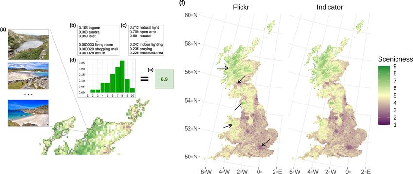
www.nature.com/scientificreports/
peoples’ individual interactions with the environment, an important methodological factor from an ES model-
ling perspective19–21. Any measurements over time are also limited by updates to the underlying datasets which
can take several years, an inflexible timeframe when considering the annual accounting requirements of some
ES assessments8.
Recently, social media has emerged as a rich new source of information on human–nature interactions. The
image-sharing platform Flickr has proven to be a particularly useful source of information. The locations of
images and associated metadata, including tags and descriptions, have now been widely employed across the
ES22–26, land use27,28 and landscape research literature16,29,30. Still, the data by themselves are difficult to interpret,
mostly due to their volume and velocity. To respond to these challenges, researchers have turned to machine
learning. In particular, deep learning, which uses artificial neural networks to generate predictions31. Supported
by the increasing availability of training data and high-performance computer hardware, deep learning has made
automatic image classification and object detection tasks possible over large datasets, including social media32–35.
As a result, deep learning has been identified as an important new tool in the development of rapid, flexible and
transferable cultural ES indicators36.
In the case of landscape aesthetics, an especially relevant training dataset exists: the Scenic-Or-Not (SoN)
database. Through a web-based portal, the database has collected 1.5 million ‘scenicness’ ratings between 1 and
10 of 217,000 landscape images of Great B ritain37. The images are sourced from Geograph, an online project
to collect a geographically representative image of every square kilometre of the U.K. and Ireland. Studies have
drawn on the SoN database to independently demonstrate both the potential of social media and machine learn-
ing in understanding peoples’ aesthetic preferences. Flickr metadata has been used to generate spatial predictions
of scenic b eauty38. Geograph tags have also been used to predict scenicness with random forests, a tree-based
ensemble learning method for r egression39. More recent studies have considered the image content directly
using deep learning: image attributes related to the scenes and objects in SoN images have been used to generate
scenicness predictions40,41. Subsequent research has focused on the detection of attribute groups co-influencing
the perception of s cenicness42, the discovery of new attributes using ancillary text c orpora43, and the relationship
between scenicness and land cover as observed by remote sensing s atellites44.
These studies demonstrate the potential of modelling landscape aesthetics using social media and deep learn-
ing. At the same time, from an ES modelling perspective, social media provides the possibility of integrating
peoples’ revealed preferences through their spatial interactions with the environment, and to observe the aesthetic
contributions of landscapes with high spatial and temporal g ranularity45. This is in contrast to indicator-based
models, which only take into account a general set of stated preferences, are limited by their spatial resolution
and rely on updates to the underlying datasets to track temporal changes. Still, user activity on social media may
not reflect common aesthetic preferences and could fail to detect significant changes over time. This is because
studies validating the use of social media for cultural ES indicators are l acking46, a common problem in cultural
ES studies47. Examining the accuracy of social media and deep learning in modelling landscape aesthetics versus
an indicator-based approach will thus generate much-needed evidence confirming the potential benefits of using
these novel techniques.
In this study, we compare models of landscape quality using Flickr and deep learning with an environmental
indicator model, and explore their synergistic use. We generate spatial predictions for Great Britain using random
forests and draw on the SoN database and its concept of scenicness to train and test our models. Flickr-based
variables are generated using the predictions of two deep learning models at the image-level. The first, a pre-
trained Places365-ResNet-50 m odel48, predicts scene classes and image attributes using the SUN database49. A
scene class can be defined as the overall semantic description of an image while an image attribute is a specific
characteristic within it (e.g. a collection of objects or human activity). The second model, a SoN ResNet, generates
scenicness predictions in individual images. Environmental indicator variables are linked to visual concepts in the
literature and are calculated using ecosystem type maps of Europe and other open-source data. We also analyse
the effect of limiting Flickr user activity and examine aesthetic enjoyment over time in national park areas. Our
findings illustrate how these innovative methods can advance ES modelling to achieve sustainable policy goals.
Results
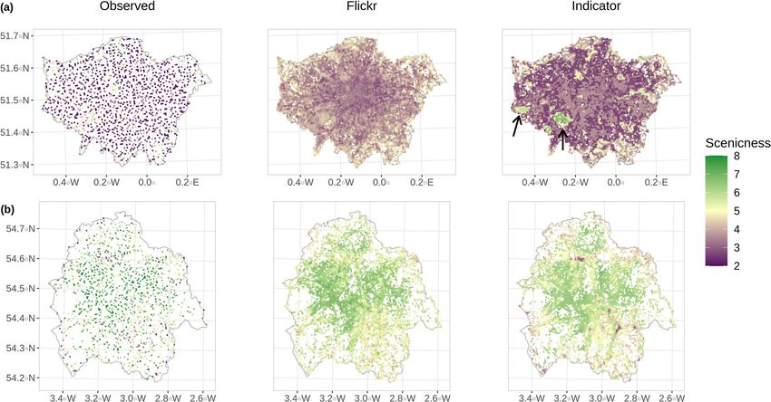
Scenicness predictions using Flickr images and deep learning. An example of a Flickr and deep learning-based
prediction for a single 5 × 5 km grid cell is shown in Fig. 1. Individual Flickr images (Fig. 1a) are passed through
the Places365-ResNet-50 model to generate a grid cell mean for 365 scene classes (Fig. 1b) and 102 SUN image
attributes scores (Fig. 1c), while image scenicness scores generated by the SoN ResNet are used to produce a nor-
malised rating distribution between 1 and 10 (Fig. 1d). The scene class and image attribute scores show that, on
average, the Places365-ResNet-50 model scored the images in the grid cell the highest for the “lagoon”, “tundra”
and “islet’ scenes, and the lowest for “atrium”, “shopping mall” and “living room”. In terms of attributes, the images
were scored the highest for “natural light”, “open area” and “natural” while “enclosed area”, “praying” and “indoor
lighting” received the lowest scores. A full list of image attribute and scene classes is available in Supplementary
Tables S1 and S2 online. The normalised rating distribution shows that most images were rated 7 and above by the
SoN ResNet. The predictions produced by the two deep learning models were then used as individual variables
in a random forest model which predicted a final scenicness score of 6.9 for the grid cell (Fig. 1e).
Comparison of Flickr, environmental indicator and combined models. The accuracy of the random forest mod-
els using the Flickr and deep learning-based variables, environmental indicators, and different combinations of
the two, within a 20% hold-out test area are show in Table 1. Accuracy is reported using r 2, root mean squared
error (RMSE) and Kendall’s τ , a ranking correlation coefficient between − 1 (inverse correlation) and 1 (absolute
correlation). Using Kendall’s τ to rank the models, the best-performing Flickr model used the Places365 scene
classes and SUN attributes as variables. The model achieved a τ of 0.683 versus 0.730 achieved by the indicator
Scientific Reports | (2021) 11:20000 | https://doi.org/10.1038/s41598-021-99282-0 2
Vol:.(1234567890)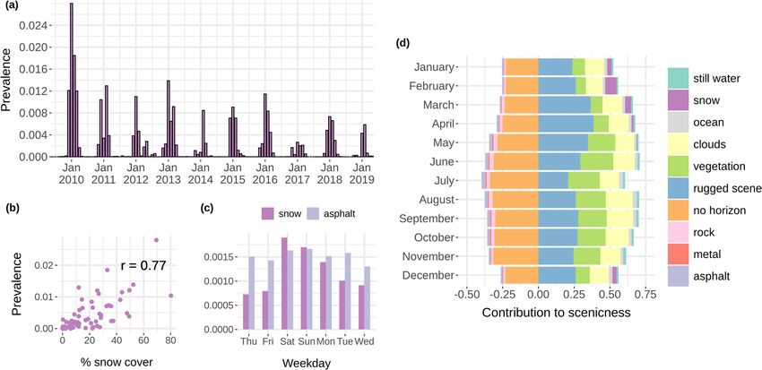
www.nature.com/scientificreports/
Figure 1. A Flickr and deep learning-based prediction of scenicness at 5 km resolution for a single cell covering
Achmelvich Bay, Scotland, and for Great Britain, in comparison to the indicator model. The deep learning-based
models used (a) Flickr images to generate (b) 365 scene class scores and (c) 102 SUN attribute scores, as well as
(d), a normalised scenic rating distribution. These were then used to build a random forest model to generate
(e) a scenicness prediction. In (f), predictions of the best-performing Flickr model for Great Britain are shown
alongside the indicator model. From top to bottom, the arrows point to the Scottish Highlands, Glasgow, the
Lake District, Snowdonia National Park and London. Drawn using R 3.6.3. (https://www.r-project.org/) with
the ggplot2 3.3.5 (https://ggplot2.tidyverse.org) and cowplot 1.1.0 (https://cran.r-project.org/package=cowplot
packages). Photos © Sergio and © Graeme Churchard (cc-by/2.0).
Scenic rating Environmental
Model Places365 scene classes SUN attributes distribution indicators r2 RMSE Kendall’s τ
Flickr
1 – – ✓ – 0.659 0.639 0.611
2 – ✓ – – 0.754 0.542 0.671
3 – ✓ ✓ – 0.757 0.540 0.672
4 ✓ – – – 0.757 0.541 0.677
5 ✓ – ✓ – 0.757 0.541 0.677
6 ✓ ✓ ✓ – 0.766 0.529 0.680
7 ✓ ✓ – – 0.770 0.525 0.683
Indicator
8 – – – ✓ 0.819 0.468 0.730
Combination
9 ✓ ✓ – ✓ 0.827 0.458 0.732
10 ✓ ✓ ✓ ✓ 0.827 0.457 0.733
11 – ✓ – ✓ 0.830 0.453 0.734
12 ✓ – – ✓ 0.832 0.453 0.738
13 – – ✓ ✓ 0.830 0.453 0.739
Table 1. Scenicness model accuracy results on the gridded test set at 5 km resolution, derived from the SoN
database.
model. Model performance was maximised when the environmental indicator variables and the scenic rating
distribution were combined, producing a τ of 0.739.
The spatial predictions generated by the best-performing Flickr model and indicator model for the whole of
Great Britain at 5 km grid cell resolution are shown in Fig. 1f. The two model types produced very similar spa-
tial predictions. Areas of particularly high aesthetic value are captured well by both models, such as Snowdonia
National Park in Wales, the Lake District in England and the Scottish Highlands. Similarly, urban areas of less
scenic quality such as London in England and Glasgow in Scotland, are also clearly visible. In Fig. 2, a more
detailed comparison is shown of the model predictions at 500m resolution versus the observed values. In both
the Greater London area (Fig. 2a) and in the Lake District (Fig. 2b), we see more nuanced predictions using the
Scientific Reports | (2021) 11:20000 | https://doi.org/10.1038/s41598-021-99282-0 3
Vol.:(0123456789)www.nature.com/scientificreports/
Figure 2. Observed scenicness versus the spatial predictions generated by the best-performing Flickr model
and indicator model at 500 m resolution in (a) the Greater London area and (b) the Lake District national park.
The arrows within the Greater London indicator model map point to Heathrow Airport (left) and Richmond
Park (right). The observed versus predicted grid cell values are shown in Supplementary Fig. S1 online. Drawn
using R 3.6.3 (https://www.r-project.org/) with the ggplot2 3.3.5 (https://ggplot2.tidyverse.org) and cowplot
1.1.0 (https://cran.r-project.org/package=cowplot) packages.
(a) Flickr (b) Indicator (c) Combination
climbing I1 farmland I1 farmland
rugged scene J1 cities, towns, villages relief
rock relief E2 mesic grasslands
valley J2 low density buildings J1 cities, towns, villages
mountain E2 mesic grasslands J2 low density buildings
glacier F3 montane shrub (s) 8
parking garage/outdoor D1 bogs 2
corn field G3 coniferous woodland 7
tundra F2 alpine shrub (s) 3
islet F3 montane shrub F3 montane shrub (s)
lagoon F4 heathland shrub (s) D1 bogs
boating J4 roads G3 coniferous woodland
natural H3 inland cliffs (s) F4 heathland shrub (s)
swimming G1 deciduous woodland 9
hiking PD F3 montane shrub
tree farm J3 extractive sites (s) H3 inland cliffs (s)
diving G4 mixed woodland (s) PD
still water E1 dry grasslands (s) J4 roads
ocean H5 sparse vegetation (s) F2 alpine shrub (s)
subway station/platform SDI J3 extractive sites (s)
0 10 20 30 40 50 60 70 80 90100 0 10 20 30 40 50 60 70 80 90100 0 10 20 30 40 50 60 70 80 90100
Variable importance Variable importance Variable importance
Figure 3. Most important variables for (a) the best-performing Flickr model, (b) environmental indicator
model, and (c) best-performing combination model at 5 km resolution. “(s)” denotes an ecosystem in
surrounding area variable. Supplementary Table S3 online contains a full list of ecosystem type codes and class
descriptions. Drawn using R 3.6.3 (https://www.r-project.org/) and the ggplot2 3.3.5 (https://ggplot2.tidyverse.
org) package.
Flickr model, while the indicator model produces more extreme values and sharp boundaries. For example, in
Greater London, Richmond Park and Heathrow Airport are predicted as very scenic areas in contrast to some of
the neighbouring areas by the indicator model, while the predictions of the Flickr model are much more muted
and in line with the observed values. In the Lake District, we also see more extreme values in the unscenic areas
using the indicator model, while the Flickr model behaves again in a more conservative manner. Overall, the
Flickr model predictions in both areas show more consistency with the observed values, although the least scenic
areas in the Lake District are less visible.
Variable importance for the Flickr, environmental indicator and combination models at 5 km resolution are
shown in Fig. 3. The best-performing Flickr model, which used the Places365 scene classes and SUN attributes as
variables, mainly drew on “climbing” and “rugged scene” in making its predictions. Natural scenes and attributes
closely related to landscape aesthetics were also prominent such as “valley”, “mountain” and “natural”, as well as
other recreation-related attributes such as “hiking”. The indicator model relied heavily on the presence of arable
Scientific Reports | (2021) 11:20000 | https://doi.org/10.1038/s41598-021-99282-0 4
Vol:.(1234567890)www.nature.com/scientificreports/
0.004
Score difference
0.000
−0.004
−0.008
−0.012
r li on
ind y h uds
oc g
bo n
tra nat ng
clo or l
se ting
im a
ion
ra ing
su d
fol ny
ex iage
h se
ge on
pla ing
s
mp r t s
g
gr h
en nsp ura
as
tin
ea
sw are
a
yin
t
clo
n
no erci
oo oriz
ve oriz
ati
ilro
co spo
tat
m
et
a lo
gh
d
aw c
−
far
Image attribute
Figure 4. The largest differences in image attribute scores after limiting Flickr user contributions. To calculate
the difference, a single image per user per day per grid cell was randomly selected ten times and the mean
attribute scores were calculated per grid cell. The median difference versus the unfiltered dataset is shown here
with summary statistics available in Supplementary Table S5 online. Drawn using R 3.6.3 (https://www.r-project.
org/) and the ggplot2 3.3.5 (https://ggplot2.tidyverse.org) package.
land and market gardens (I1), relief, and the presence of buildings (J1 and J2) to generate a scenicness prediction.
This was followed by the presence of natural ecosystems, including grasslands (E2), mires/bogs (D1), heathland
(F3s, F4s and F3), and inland scree/bare surfaces (H3s). The complexity indices SDI and PDI did not constitute
important variables. The best-performing combined model, incorporating the scenic rating distribution (model
13, Table 1), drew on a similar set of indicator variables and the more extreme scenic ratings, focusing on the
distributions across rating bins 2, 3, 7 and 8.
Limiting Flickr user activity. For ES modelling purposes at national level, it is important to capture a repre-
sentative measure of ecosystem contributions to human well-being. In the case of the Flickr models, accuracy
results are reported after limiting individual Flickr users to one image per day per 5 × 5 km grid cell. We applied
the limitation after finding large geographic disparities in images per user (Supplementary Fig. S2 online).
After applying the limitation, model accuracy improved versus a non-filtered dataset (Supplementary Table S4
online). Figure 4 shows the largest resulting change in image attribute confidence scores. A key change that can
be observed is a decrease in the prevalence of images related to sporting. For example, “playing”, “competing”,
“sports”, and “exercise” all saw notable decreases. This suggests that a large number of images associated with
sporting events, less relevant for measuring landscape aesthetics, were removed from the dataset by the filtering.
This in turn appears to have increased the prevalence of landscape-focused imagery, indicated by the increase in
confidence scores for the “clouds”, “far-away horizon”, “ocean” and “natural” attributes.
Measuring changes in aesthetic enjoyment over time. Deep learning-based variables generated using social
media can also support measures of landscape aesthetics over time. This can support more frequent updates to
national ES assessments, and tell us more about how the landscape is contributing to peoples’ well-being. In an
additional experiment aiming at studying the temporal dynamics of peoples’ aesthetic enjoyment through their
interactions with the landscape, we analysed how scenicness evolves over time in national park areas. Figure 5
shows the contributions of a selected group of image attributes over a ten year period within the 15 national
parks of Great Britain. These contain some of the most valuable natural areas in Britain, such as the Peak and
Lake Districts in England, the Pembrokeshire coast in Wales, and the Cairngorms in Scotland.
The contribution of aesthetic-related image attributes change in these national parks according to the season.
We focus on the “snow” attribute as a specific example of how these contributions change over time. Figure 5a
shows how the prevalence of “snow”, the average score accounting only for images with a score higher than 0.5,
increases in the winter months. The winter of 2009/2010 reveals itself as a particularly snowy period. The preva-
lence of snow in user images correlates strongly with remote sensing-based measurements of snow cover using
MODIS satellite data, shown in Fig. 5b. In Fig. 5c, we also see how the prevalence of “snow” increases around
the weekend when people are more likely to visit snowy landscapes, whilst the prevalence of “asphalt” in images
remains relatively constant throughout the week. This shows that the use of social media-based data provides a
combination of information about the state of the environment and how people interact with it.
In a direct connection to aesthetic landscape quality, when the selected group of image attributes shown in
Fig. 5d, including “snow”, are used to predict the image ratings generated by the SoN ResNet, we see again how
the contributions change over time. For example, the contributions of “snow” appear between December and
April, reaching a peak in the winter month of February, before disappearing again. In contrast, the contributions
of “vegetation” grow to their highest between June and August, reflecting the positive influence of deciduous
growth on landscape aesthetics in the summer. Although smaller in size, the contributions of “ocean” also grow
in the summer, suggesting an increase in user posts of coastal images to Flickr in these warmer months. It is also
notable that the contribution of “rugged scene” to scenicness increases in the rainy months of spring.
Scientific Reports | (2021) 11:20000 | https://doi.org/10.1038/s41598-021-99282-0 5
Vol.:(0123456789)www.nature.com/scientificreports/
Figure 5. The influence of “snow” and other image attributes on aesthetic enjoyment over time. The (a) average
monthly prevalence of “snow” attribute scores > 0.5 are shown between 2009 and 2019. The average monthly
scores show a strong correlation (Pearson’s R = 0.77) with (b) remotely-sensed snow cover data. The (c) average
prevalence per weekday of “snow” versus “asphalt” is also shown. A constrained linear model (R2 = 0.34) was
trained using the scores > 0.5 of a selected group of attributes including “snow” to (d) predict scenicness at
the image-level. The changing monthly contributions of some of these attributes can be observed, with “snow”
contributing in the winter months. Contributions represent individual image attribute scores multiplied by the
model coefficients and averaged on a monthly basis. Drawn using R 3.6.3 (https://www.r-project.org/) with the
ggplot2 3.3.5 (https://ggplot2.tidyverse.org) and cowplot 1.1.0 (https://cran.r-project.org/package=cowplot)
packages.
Discussion
The potential of social media and deep learning to capture peoples’ interactions with the landscape has yet to
be fully confirmed. In an ES context, social media provides a rich new source of data to capture the cultural
contributions of ecosystems to human well-being but its use is rarely v alidated46. In the ES community, deep
learning applications also remain limited and those that do exist tend to limit their analysis to using the objects
detected in images as proxies for cultural E S25,36,50. We have demonstrated that deep learning-based variables
which consider the overall semantic meaning of an image can accurately capture the aesthetic quality of the Brit-
ish landscape. Crucially, these techniques also incorporate peoples’ actual interactions with the environment, a
key methodological requirement from an ES perspective.
Nevertheless, our study highlights the relevance of traditional environmental indicator models in capturing
landscape quality in the absence of survey data. The visual concepts put forward in the landscape aesthetics
literature serve well to capture the spatial variation in scenicness provided by the SoN database. The especially
strong influence of unnatural, man-made environments on aesthetics is reflected in the high variable importance
of arable land and b uildings51. At the same time, the importance of highly valued and unique natural environ-
ments, such as bog and heathland ecosystems, as well as the importance of relief, are also accurately identified by
the random forest model52–54. Surprisingly, the SDI and PDI, normally key indicators for measuring landscape
aesthetics55 and relevant to Britain56, did not constitute important variables in our results. The variety of ecosys-
tem type indicators and their interaction in the non-linear model space may have offered enough opportunities
to capture landscape complexity57. Alternatively, visibility modelling of the landscape could produce a more
accurate set of indicators21,58,59. Theoretically, these could capture more of the aesthetic quality of the landscape
by providing a 3D perspective using the location of Flickr images. However, the challenge with visibility model-
ling at very large scales is the computational resources needed for the geo-spatial c alculations60. For example, in
our case, the sightlines from 9.8 million images would need to be calculated using a 25 × 25 m Digital Elevation
Model (DEM) for a 210,000 km2 area. On the other hand, in the case of our Flickr model, the presence of image
attributes including “far-away horizon” and scene classes such as “mountain” give the model a lot of indirect
information on the 3D characteristics of an area.
The inclusion of individual spatial interactions offered by the Flickr and deep learning-based approach also
makes it a more attractive method for ES modelling purposes. The comparable model accuracy versus the indica-
tor model shows that this key methodological requirement from an ES perspective can be incorporated without
significant losses in accuracy. The results also show that this individual perspective produces a finer-grained view
which captures highly-valued and unique landscape elements such as rock or water features18. For example, the
highly aesthetic view of Achmelvich Bay in Scotland, shown in Fig. 1. This is in contrast to the indicator model,
which uses variables measured with remote sensing data at 25 m resolution and above. At the same time, impor-
tant negative environmental contexts, such as Heathrow Airport in London (Fig. 2), are also better captured by
the Flickr model. Figure 2 also shows how the Flickr model stays relevant at different scales while simultaneously
Scientific Reports | (2021) 11:20000 | https://doi.org/10.1038/s41598-021-99282-0 6
Vol:.(1234567890)www.nature.com/scientificreports/
highlighting the scaling issues common to indicator models61. While the indicator model is heavily constrained
by the scale of measurement, producing more extreme differences linked to land cover, the Flickr model is able
to reproduce a more consistent view of the landscape using the images available to it (see also Supplementary
Fig. S1 online). At a national level, it appears that explicitly capturing this more nuanced view of the landscape
through the scenic rating distribution, in combination with the strong overall predictive power of the indicator
model, produces the highest level of model accuracy in our study.
In contrast to the static nature of the indicator approach, the granularity of the Flickr data also enables a
detailed examination of aesthetics over time. The time-series analysis illustrated in Fig. 5 shows how the aesthetic
contributions of landscapes change over the course of a year in the national parks of Britain. The influence of
seasonality on landscape quality, defined as ‘ephemera’ in the landscape aesthetics l iterature17, is notably captured.
Such granularity can greatly benefit ES assessments requiring regular updates, such as those performed for the
purposes of ecosystem accounting in the context of national annual accounts of economic production8. These
results also show how the contributions of specific landscape characteristics to peoples’ aesthetic enjoyment can
be accurately captured using a social media and deep learning-based approach. The large prevalence of snow
in images during the 2009/2010 winter is consistent with one of the last great snowfall events in B ritain62. The
consistency with remote sensing data further supports the reliability of the data. Understanding how ecosystems
in the landscape contribute to individuals’ aesthetic enjoyment of the landscape, and accurately tracking these
contributions over time, can help policy-makers manage and protect the most valuable natural areas for peoples’
recreation and well-being.
Although the Flickr and deep learning approach has its advantages, some biases in the method should still
be taken into account. By using the SoN database for training purposes, the models have largely learnt a Brit-
ish representation of aesthetic quality. For applications in other cultural and topographical contexts, additional
fine-tuning will most likely be required. Challenges also lie in trying to gain an ES measure demographically-
representative of the entire population. Flickr has been found to be the most popular with 40 to 60 year-old
males63 and user contributions, as in our study, are usually skewed by small, highly active user groups64. At the
same time, a great number of differences in the content of images exist and not all images are relevant for meas-
uring landscape aesthetics. However, in this respect, the user limitation in our study appears to have shifted the
overall image content away from sporting scenes and more towards landscape images, improving model accuracy
versus the SoN database. Notably, the agreement between the Flickr-based models, SoN and the environmental
indicators shows that there is a strong consistency between the preferences captured by each dataset. This consist-
ency is also promising for applications in other European contexts as the aesthetic concepts used to develop the
environmental indicators have already been successfully applied in a number of European settings65.
In conclusion, landscape aesthetics are an important source of cultural value but large-scale measurement
for ES assessments is difficult due to a lack of survey data. Now, social media offers the opportunity to measure
the aesthetic contributions of ecosystems whilst integrating peoples’ actual interactions with the environment,
and tracking changes over time. In this study, we have demonstrated that models using Flickr images and deep
learning enable a highly accurate measure of aesthetic landscape quality, with independence of the scale of meas-
urement. This supports ES measures based on the revealed preferences of individuals rather than a set of broad
theoretical concepts. Small gains in accuracy are also achieved when an explicit, deep learning-based measure
of aesthetics in the form of an image rating distribution is combined with environmental indicator variables.
Changes in the aesthetic contributions of landscapes over time can also be measured. Our results advance ES
modelling to better capture the cultural contributions of nature to human well-being.
Methods
Study design. The research focused on comparing Flickr and deep learning-based models with an environmental
indicator-based model, as well as different combinations of the two (Fig. 6). Conceptually, we considered the
aesthetic quality of the landscape equivalent to the concept of scenicness, and that scenicness constituted an
integral factor determining the overall flow of aesthetic E S66. We made our comparisons using a 5 × 5 km grid
covering the entire terrestrial area of Great Britain and at 500 m resolution in Greater London and the Lake
District. As a ground truth, we calculated a mean scenicness rating per grid cell using the image scenicness rat-
ings of intersecting SoN images. Each image has a collection of volunteer ratings between 1 (not scenic) and 10
(very scenic). We used the average of these ratings. For training, we used the 5 km × 5 km grid. To reduce spatial
autocorrelation, a larger 50 × 50 km grid was then overlaid onto this grid to create sample groups of which 70%
was randomly allocated for training, 10% for validation and 20% for testing (Supplementary Fig. S3 online).
Random forests was used to model scenicness at the 5 km and 500 m grid level using both the environmental
indicator and Flickr-based variables. All spatial analyses were done using the R 3.6.3 programming language
(https://www.r-project.org/) including the raster 3.0–12 (https://cran.r-project.org/package=raster), sf 1.0-1
(https://cran.r-project.org/package=sf), caret 6.0–86 (https://cran.r-project.org/package=caret) and tidyverse
1.3.1 (https://cran.r-project.org/package=tidyverse) packages. caret was used to automatically select the random
forest hyperparameter settings mtry, min node size, and extratrees.
Datasets. In addition to the SoN database, a Flickr image dataset was compiled to generate the deep learning-
based variables. To do this, image metadata for geo-located images taken in Great Britain between 2004 and 2020
were downloaded using Flickr’s API and accessed using the Python programming language. A script was devel-
oped which iterated over a 1 × 1 km grid, requesting the metadata of the 4000 most recent, geo-located images
per grid cell. Geo-location accuracy was set to “street level”, the highest possible accuracy available through the
API. The Places365-ResNet-50 model48 was then used to filter the dataset for outdoor images using its binary
indoor/outdoor scene predictions. This resulted in a final dataset of 9.8 million outdoor images, resized to 250 ×
250 pixel dimensions. The environmental indicator variables were also calculated using a number of geospatial
Scientific Reports | (2021) 11:20000 | https://doi.org/10.1038/s41598-021-99282-0 7
Vol.:(0123456789)www.nature.com/scientificreports/
(a) Flickr and deep learning-based models
mean
score
Places365
ResNet-50
5x5km
grid cell 102 SUN 365 Places
Random
attributes scene classes 6.8
forest
SoN image rating
distribution
ResNet
1 2 3 4 5 6 7 8 9 10
(b) Environmental indicator model (c) Combined
Ecosystem models
type map
Random Random
DEM 6.7 6.9
forest forest
Historic
POI environmental
indicators
Figure 6. The main study design comparing spatial predictions of scenicness at a 5 × 5 km grid cell resolution
using random forests. These used different combinations of variables based on (a) the predictions of two deep
learning models on Flickr images, (b) a set of environmental indicators, and (c) combinations of the two. Photos
© Alun Ward (cc-by/2.0).
datasets (Supplementary Table S6 online). These included the European Environment Agency (EEA) ecosystem
type map, the EU DEM and OpenStreetMap. The EU GDPR on data protection and privacy were followed in
the carrying out of the research.
Flickr and deep learning-based variables. To model scenicness at the grid level, spatial variables were gener-
ated using two deep learning models developed in Python 3.8.3 (Fig. 6). The pre-trained Places365-ResNet-50
model48 was applied to Flickr images to produce a first set of variables: a mean of 365 scene classes and 102 SUN
image attribute scores per grid cell (a complete list is available in Supplementary Tables S1 and S2 online). Scene
classes capture the overall semantic interpretation of an image, with scores representing probabilities between
0 and 1 based on the most likely scene out of 365 scene classes. Image attribute scores indicate the presence of
objects and remarkable scene characteristics. These were normalised using a sigmoid function to produce a 0–1
probability per attribute. The second model, the SoN ResNet, was used to predict scenicness in Flickr images
and to generate a second set of variables: a normalised count of its image predictions across ten scenic rating
bins between 1 and 10, representing a scenic rating distribution per grid cell. We constructed this model using
a modified ResNet-50 convolutional neural network, available pre-trained on the ImageNet database through
the PyTorch 1.6.0 library. The final two layers of the network, originally designed to output confidence scores for
ImageNet’s 1000 object classes, were removed and replaced with new layers designed to output an image scenic-
ness score42. These consisted of an adaptive average pooling layer and two linear layers with a ReLU activation
function on the output of the first linear layer. The network was trained and tested using SoN images according
to the 70% training, 10% validation and 20% test areas. For training, this consisted of 152,470 images resized to
500 × 500 pixel dimensions. Images were also randomly flipped horizontally to increase the size of the training
dataset. Batch size was set to 16. Model weights were optimised using stochastic gradient descent and a mean
squared error loss function. Test statistics are shown in Supplementary Table S7 online.
Environmental indicator variables. Variables were calculated per grid cell based on visual preference concepts
put forward in the landscape aesthetics literature. The EEA ecosystem type map was used to calculate the per-
centage of different ecosystems to capture the naturalness of the landscape; relief in m was measured using the
EU DEM to capture the aesthetic appeal of higher elevation areas and elevation differences; the PDI and SDI
were calculated using the EEA ecosystem type map to measure landscape complexity; and, finally, to capture
the uniqueness of natural environments and cultural elements in the landscape, the relative difference in the
percentage area of ecosystems within 10 km was calculated, as well as the number of historical points of interest
(POI) using OSM (Fig. 6). More details on the theoretical basis for these indicators and their calculation can be
found in Supplementary Table S6 online.
Environmental indicator reduction. To improve model performance and interpretability, the initial environ-
mental indicator set was reduced. First, ecosystem variables that could be calculated for less than 100km2 or
0.04% of Great Britain were removed using a threshold analysis (Supplementary Fig. S4 online). Then, a check
for collinearity between the remaining variables was performed. The model accuracy effect of removing variables
with a correlation r ≥ 0.7 was measured through a leave-one-out process in which random forest models were
iteratively generated without one of the indicator variables in the full indicator set. The collinear variable with
the smallest effect on model accuracy was removed (Supplementary Table S8 and Fig. S5 online). This resulted
in a final indicator set of 41 variables.
Scientific Reports | (2021) 11:20000 | https://doi.org/10.1038/s41598-021-99282-0 8
Vol:.(1234567890)www.nature.com/scientificreports/
Time-series analysis. An additional experiment was conducted to examine landscape aesthetics over time
in the 15 national parks of Great Britain (Supplementary Fig. S6 online). Flickr images within these areas were
extracted for the time period June 2009 to May 2019. The image attribute scores were extracted using the
Places365-ResNet-50 model and prevalence was calculated on an image-level basis by taking only attribute scores
greater than 0.5, subtracting 0.5 and multiplying by 2. All other values were set to 0. The linear model was trained
and tested using a random 80/20% sample of images. MODIS snow cover data used the MOD10CM product
which reports monthly average snow cover in 0.05◦ . The centroids of the intersecting 5 × 5 km grid cells with
national parks were used to extract percentage snow cover on a monthly basis. Additional spatial data sources
are given in Supplementary Table S9 online.
Data availability
The data used in this study are open-source and publicly available. Code and data associated with this study can
be obtained at https://doi.org/10.5281/zenodo.5534028.
Received: 7 April 2021; Accepted: 13 September 2021
References
1. Daniel, T. C. et al. Contributions of cultural services to the ecosystem services agenda. Proc. Natl. Acad. Sci. USA 109, 8812–8819.
https://doi.org/10.1073/pnas.1114773109 (2012).
2. Gobster, P. H., Nassauer, J. I., Daniel, T. C. & Fry, G. The shared landscape: What does aesthetics have to do with ecology?. Landsc.
Ecol. 22, 959–972. https://doi.org/10.1007/s10980-007-9110-x (2007).
3. Abraham, A., Sommerhalder, K. & Abel, T. Landscape and well-being: A scoping study on the health-promoting impact of outdoor
environments. Int. J. Public Health 55, 59–69. https://doi.org/10.1007/s00038-009-0069-z (2010).
4. Rice, W. L. et al. Changes in recreational behaviors of outdoor enthusiasts during the COVID-19 pandemic: Analysis across urban
and rural communities. J. Urban Ecol. https://doi.org/10.1093/jue/juaa020 (2020).
5. Venter, Z. S., Barton, D. N., Gundersen, V., Figari, H. & Nowell, M. Urban nature in a time of crisis: Recreational use of green space
increases during the COVID-19 outbreak in Oslo, Norway. Environ. Res. Lett. 15, 104075. https://doi.org/10.1088/1748-9326/
abb396 (2020).
6. Maes, J. et al. Mainstreaming ecosystem services into EU policy. Curr. Opin. Environ. Sustain. 5, 128–134. https://d oi.o
rg/1 0.1 016/j.
cosust.2013.01.002 (2013).
7. Paracchini, M. L. et al. Mapping cultural ecosystem services: A framework to assess the potential for outdoor recreation across
the EU. Ecol. Indic. 45, 371–385. https://doi.org/10.1016/j.ecolind.2014.04.018 (2014).
8. Hein, L. et al. Progress in natural capital accounting for ecosystems. Science 367, 514–515. https://doi.org/10.1126/science.aaz89
01 (2020).
9. Díaz, S. et al. Assessing nature’s contributions to people. Science 359, 270–272. https://doi.org/10.1126/science.aap8826 (2018).
10. Martínez-Harms, M. J. & Balvanera, P. Methods for mapping ecosystem service supply: A review. Int. J. Biodiv. Sci. Ecosyst. Serv.
Manag. 8, 17–25. https://doi.org/10.1080/21513732.2012.663792 (2012).
11. Raymond, C. M., Kenter, J. O., Plieninger, T., Turner, N. J. & Alexander, K. A. Comparing instrumental and deliberative paradigms
underpinning the assessment of social values for cultural ecosystem services. Ecol. Econ. 107, 145–156. https://doi.org/10.1016/j.
ecolecon.2014.07.033 (2014).
12. Bateman, I. J. et al. Bringing ecosystem services into economic decision-making: Land use in the United Kingdom. Science 341,
45–50. https://doi.org/10.1126/science.1234379 (2013).
13. Hernández-Morcillo, M., Plieninger, T. & Bieling, C. An empirical review of cultural ecosystem service indicators. Ecol. Indic. 29,
434–444. https://doi.org/10.1016/j.ecolind.2013.01.013 (2013).
14. Hermes, J., Albert, C. & von Haaren, C. Assessing the aesthetic quality of landscapes in Germany. Ecosyst. Serv. 31, 296–307. https://
doi.org/10.1016/j.ecoser.2018.02.015 (2018).
15. Uuemaa, E., Antrop, M., Roosaare, J., Marja, R. & Mander, U. Landscape metrics and indices: An overview of their use in landscape
research. Living Rev. Landsc. Res. 3, 1–28. https://doi.org/10.12942/lrlr-2009-1 (2009).
16. Schirpke, U., Tasser, E. & Tappeiner, U. Predicting scenic beauty of mountain regions. Landsc. Urban Plan. 111, 1–12. https://doi.
org/10.1016/j.landurbplan.2012.11.010 (2013).
17. Tveit, M., Ode, Å. & Fry, G. Key concepts in a framework for analysing visual landscape character. Landsc. Res. 31, 229–255. https://
doi.org/10.1080/01426390600783269 (2006).
18. Ode, Å., Tveit, M. & Fry, G. Capturing landscape visual character using indicators: Touching base with landscape aesthetic theory.
Landsc. Res. 33, 89–117. https://doi.org/10.1080/01426390701773854 (2008).
19. de Groot, R. S., Alkemade, R., Braat, L., Hein, L. & Willemen, L. Challenges in integrating the concept of ecosystem services and
values in landscape planning, management and decision making. Ecol. Complex. 7, 260–272. https://doi.org/10.1016/j.ecocom.
2009.10.006 (2010).
20. Schröter, M., Remme, R. P., Sumarga, E., Barton, D. N. & Hein, L. Lessons learned for spatial modelling of ecosystem services in
support of ecosystem accounting. Ecosyst. Serv. 13, 64–69. https://doi.org/10.1016/j.ecoser.2014.07.003 (2015).
21. Tenerelli, P., Püffel, C. & Luque, S. Spatial assessment of aesthetic services in a complex mountain region: Combining visual
landscape properties with crowdsourced geographic information. Landsc. Ecol. 32, 1097–1115. https://doi.org/10.1007/s10980-
017-0498-7 (2017).
22. Wood, S. A., Guerry, A. D., Silver, J. M. & Lacayo, M. Using social media to quantify nature-based tourism and recreation. Sci. Rep.
3, 1–7. https://doi.org/10.1038/srep02976 (2013).
23. van Zanten, B. T. et al. Continental-scale quantification of landscape values using social media data. Proc. Natl. Acad. Sci. USA
113, 12974–12979. https://doi.org/10.1073/pnas.1614158113 (2016).
24. Tenerelli, P., Demšar, U. & Luque, S. Crowdsourcing indicators for cultural ecosystem services: A geographically weighted approach
for mountain landscapes. Ecol. Indic. 64, 237–248. https://doi.org/10.1016/j.ecolind.2015.12.042 (2016).
25. Richards, D. R. & Tunçer, B. Using image recognition to automate assessment of cultural ecosystem services from social media
photographs. Ecosyst. Serv. 31, 318–325. https://doi.org/10.1016/j.ecoser.2017.09.004 (2018).
26. Sinclair, M., Mayer, M., Woltering, M. & Ghermandi, A. Valuing nature-based recreation using a crowdsourced travel cost method:
A comparison to onsite survey data and value transfer. Ecosyst. Serv. 45, 101165. https://doi.org/10.1016/j.ecoser.2020.101165
(2020).
27. Antoniou, V. et al. Investigating the feasibility of geo-tagged photographs as sources of land cover input data. ISPRS Int. J. Geo-
Inf.https://doi.org/10.3390/ijgi5050064 (2016).
Scientific Reports | (2021) 11:20000 | https://doi.org/10.1038/s41598-021-99282-0 9
Vol.:(0123456789)www.nature.com/scientificreports/
28. Mancini, F., Coghill, G. M. & Lusseau, D. Quantifying wildlife watchers’ preferences to investigate the overlap between recreational
and conservation value of natural areas. J. Appl. Ecol. 56, 387–397. https://doi.org/10.1111/1365-2664.13274 (2019).
29. Hollenstein, L. & Purves, R. Exploring place through user-generated content: Using Flickr tags to describe city cores. J. Spatial Inf.
Sci. 1, 21–48. https://doi.org/10.5311/JOSIS.2010.1.3 (2010).
30. Donahue, M. L. et al. Using social media to understand drivers of urban park visitation in the Twin Cities, MN. Landsc. Urban
Plan. 175, 1–10. https://doi.org/10.1016/j.landurbplan.2018.02.006 (2018).
31. LeCun, Y., Bengio, Y. & Hinton, G. Deep learning. Nature 521, 436–444. https://doi.org/10.1038/nature14539 (2015).
32. Naik, N., Kominers, S. D., Raskar, R., Glaeser, E. L. & Hidalgo, C. A. Computer vision uncovers predictors of physical urban change.
Proc. Natl. Acad. Sci. USA 114, 7571–7576. https://doi.org/10.1073/pnas.1619003114 (2017).
33. Toivonen, T. et al. Social media data for conservation science: A methodological overview. Biol. Conserv. 233, 298–315. https://
doi.org/10.1016/j.biocon.2019.01.023 (2019).
34. Zhang, F., Zhou, B., Ratti, C. & Liu, Y. Discovering place-informative scenes and objects using social media photos. R. Soc. Open
Sci. 6, 181375. https://doi.org/10.1098/rsos.181375 (2019).
35. Srivastava, S., Vargas Muñoz, J. E., Lobry, S. & Tuia, D. Fine-grained landuse characterization using ground-based pictures: A deep
learning solution based on globally available data. Int. J. Geogr. Inf. Sci. 34, 1117–1136. https://doi.org/10.1080/13658816.2018.
1542698 (2020).
36. Egarter Vigl, L. et al. Harnessing artificial intelligence technology and social media data to support cultural ecosystem service
assessments. People Nat. 3, 673–685. https://doi.org/10.1002/pan3.10199 (2021).
37. ScenicOrNot. ScenicOrNot Dataset (2015). http://scenicornot.datasciencelab.co.uk.
38. Seresinhe, C. I., Moat, H. S. & Preis, T. Quantifying scenic areas using crowdsourced data. Environ. Plan. B Urban Anal. City Sci.
45, 567–582. https://doi.org/10.1177/0265813516687302 (2017).
39. Chesnokova, O., Nowak, M. & Purves, R. S. A crowdsourced model of landscape preference. In 13th International Conference on
Spatial Information Theory (COSIT 2017), vol. 86. https://doi.org/10.4230/LIPIcs.COSIT.2017.19 (2017).
40. Seresinhe, C. I., Tobias, P. & Moat, H. S. Using deep learning to quantify the beauty of outdoor places. R. Soc. Open Sci.. https://
doi.org/10.1098/rsos.170170 (2017).
41. Workman, S., Souvenir, R. & Jacobs, N. Understanding and mapping natural beauty. In 2017 IEEE International Conference on
Computer Vision (ICCV), vol. 4, 5590–5599. https://doi.org/10.1109/ICCV.2017.596 (2017).
42. Marcos, D. et al. Contextual semantic interpretability. In Proceedings of the Asian Conference on Computer Vision (2020).
43. Arendsen, P., Marcos, D. & Tuia, D. Concept discovery for the interpretation of landscape scenicness. Mach. Learn. Knowl.
Extract.https://doi.org/10.3390/make2040022 (2020).
44. Levering, A., Marcos, D. & Tuia, D. On the relation between landscape beauty and land cover: A case study in the U.K. at Sentinel-2
resolution with interpretable AI. ISPRS J. Photogram. Remote Sens. 177, 194–203. https://doi.org/10.1016/j.isprsjprs.2021.04.020
(2021).
45. Havinga, I., Bogaart, P. W., Hein, L. & Tuia, D. Defining and spatially modelling cultural ecosystem services using crowdsourced
data. Ecosyst. Serv. 43, 101091. https://doi.org/10.1016/j.ecoser.2020.101091 (2020).
46. Oteros-Rozas, E., Martín-López, B., Fagerholm, N., Bieling, C. & Plieninger, T. Using social media photos to explore the relation
between cultural ecosystem services and landscape features across five European sites. Ecol. Indic. 94, 74–86. https://doi.org/10.
1016/j.ecolind.2017.02.009 (2018).
47. Englund, O., Berndes, G. & Cederberg, C. How to analyse ecosystem services in landscapes—A systematic review. Ecol. Indic. 73,
492–504. https://doi.org/10.1016/j.ecolind.2016.10.009 (2017).
48. Zhou, B., Lapedriza, A., Khosla, A., Oliva, A. & Torralba, A. Places: A 10 million image database for scene recognition. IEEE Trans.
Pattern Anal. Mach. Intell. 40, 1452–1464. https://doi.org/10.1109/TPAMI.2017.2723009 (2017).
49. Patterson, G., Xu, C., Su, H. & Hays, J. The SUN attribute database: Beyond categories for deeper scene understanding. Int. J.
Comput. Vis. 108, 59–81. https://doi.org/10.1007/s11263-013-0695-z (2014).
50. Lee, H., Seo, B., Koellner, T. & Lautenbach, S. Mapping cultural ecosystem services 2.0—Potential and shortcomings from unlabeled
crowd sourced images. Ecol. Indic. 96, 505–515. https://doi.org/10.1016/j.ecolind.2018.08.035 (2019).
51. Ulrich, R. S. Visual landscapes and psychological well-being. Landsc. Res. 4, 17–23. https://doi.org/10.1080/01426397908705892
(1979).
52. Cordingley, J. E., Newton, A. C., Rose, R. J., Clarke, R. T. & Bullock, J. M. Habitat fragmentation intensifies trade-offs between
biodiversity and ecosystem services in a heathland ecosystem in Southern England. PLOS ONE 10, e0130004. https://doi.org/10.
1371/journal.pone.0130004 (2015).
53. Newton, A. C. et al. Impacts of grazing on lowland heathland in north-west Europe. Biol. Conserv. 142, 935–947. https://doi.org/
10.1016/j.biocon.2008.10.018 (2009).
54. Tveit, M. S. Indicators of visual scale as predictors of landscape preference; A comparison between groups. J. Environ. Manag. 90,
2882–2888. https://doi.org/10.1016/j.jenvman.2007.12.021 (2009).
55. Frank, S., Fürst, C., Koschke, L., Witt, A. & Makeschin, F. Assessment of landscape aesthetics—validation of a landscape metrics-
based assessment by visual estimation of the scenic beauty. Ecol. Indic. 32, 222–231. https://doi.org/10.1016/j.ecolind.2013.03.026
(2013).
56. Graham, L. J. & Eigenbrod, F. Scale dependency in drivers of outdoor recreation in England. People Nat. 1, 406–416. https://doi.
org/10.1002/pan3.10042 (2019).
57. Ryo, M. & Rillig, M. C. Statistically reinforced machine learning for nonlinear patterns and variable interactions. Ecosphere 8,
e01976. https://doi.org/10.1002/ecs2.1976 (2017).
58. Karasov, O., Vieira, A. A. B., Külvik, M. & Chervanyov, I. Landscape coherence revisited: GIS-based mapping in relation to scenic
values and preferences estimated with geolocated social media data. Ecol. Indic. 111, 105973. https://doi.org/10.1016/j.ecolind.
2019.105973 (2020).
59. Foltête, J.-C., Ingensand, J. & Blanc, N. Coupling crowd-sourced imagery and visibility modelling to identify landscape preferences
at the panorama level. Landsc. Urban Plan. 197, 103756. https://doi.org/10.1016/j.landurbplan.2020.103756 (2020).
60. Labib, S. M., Huck, J. J. & Lindley, S. Modelling and mapping eye-level greenness visibility exposure using multi-source data at
high spatial resolutions. Sci. Total Environ. 755, 143050. https://doi.org/10.1016/j.scitotenv.2020.143050 (2021).
61. Li, H. & Wu, J. Use and misuse of landscape indices. Landsc. Ecol. 19, 389–399. https://doi.org/10.1023/B:LAND.0000030441.
15628.d6 (2004).
62. Weather, U. K. UK seasonal weather summary—Winter 2009/2010. Weather 65, 99. https://doi.org/10.1002/wea.601 (2010).
63. Lenormand, M. et al. Multiscale socio-ecological networks in the age of information. PLOS ONE 13, e0206672. https://doi.org/
10.1371/journal.pone.0206672 (2018).
64. Li, L., Goodchild, M. F. & Xu, B. Spatial, temporal, and socioeconomic patterns in the use of Twitter and Flickr. Cartogr. Geogr.
Inf. Sci. 40, 61–77. https://doi.org/10.1080/15230406.2013.777139 (2013).
65. Uuemaa, E., Mander, Ü. & Marja, R. Trends in the use of landscape spatial metrics as landscape indicators: A review. Ecol. Indic.
28, 100–106. https://doi.org/10.1016/j.ecolind.2012.07.018 (2013).
66. Daniel, T. C. Whither scenic beauty? Visual landscape quality assessment in the 21st century. Landsc. Urban Plan. 54, 267–281.
https://doi.org/10.1016/S0169-2046(01)00141-4 (2001).
Scientific Reports | (2021) 11:20000 | https://doi.org/10.1038/s41598-021-99282-0 10
Vol:.(1234567890)You can also read