Source apportionment of fine organic carbon at an urban site of Beijing using a chemical mass balance model - Recent
←
→
Page content transcription
If your browser does not render page correctly, please read the page content below
Atmos. Chem. Phys., 21, 7321–7341, 2021
https://doi.org/10.5194/acp-21-7321-2021
© Author(s) 2021. This work is distributed under
the Creative Commons Attribution 4.0 License.

Source apportionment of fine organic carbon at an urban site
of Beijing using a chemical mass balance model
Jingsha Xu1 , Di Liu1,a , Xuefang Wu1,2 , Tuan V. Vu1,b , Yanli Zhang3 , Pingqing Fu4 , Yele Sun5 , Weiqi Xu5 , Bo Zheng6,c ,
Roy M. Harrison1,d , and Zongbo Shi1
1 School   of Geography Earth and Environmental Science, University of Birmingham, Birmingham, B15 2TT, UK
2 National  Engineering Research Center of Urban Environmental Pollution Control, Beijing Municipal Research Institute of
Environmental Protection, Beijing, 100037, China
3 Guangzhou Institute of Geochemistry, Chinese Academy of Sciences, Guangzhou, 510640, China
4 Institute of Surface-Earth System Science, Tianjin University, Tianjin, 300072, China
5 State Key Laboratory of Atmospheric Boundary Layer Physics and Atmospheric Chemistry,

Institute of Atmospheric Physics, Chinese Academy of Sciences, Beijing, 100029, China
6 State Key Joint Laboratory of Environment Simulation and Pollution Control, School of Environment,

Tsinghua University, Beijing, 100084, China
a now at: Institute of Atmospheric Physics, Chinese Academy of Sciences, Beijing, 100029, China
b now at: Faculty of Medicine, School of Public Health, Imperial College London, London, UK
c now at: Laboratoire des Sciences du Climat et de l’Environnement, CEA-CNRS-UVSQ, UMR8212, Gif-sur-Yvette, France
d also at: Department of Environmental Sciences/Center of Excellence in Environmental Studies, King Abdulaziz University,

P.O. Box 80203, Jeddah, 21589, Saudi Arabia

Correspondence: Zongbo Shi (z.shi@bham.ac.uk) and Roy M. Harrison (r.m.harrison@bham.ac.uk)

Received: 30 September 2020 – Discussion started: 3 December 2020
Revised: 23 March 2021 – Accepted: 23 March 2021 – Published: 12 May 2021

Abstract. Fine particles were sampled from 9 November to         cooking, and vegetative detritus) based on a chemical mass
11 December 2016 and 22 May to 24 June 2017 as part              balance (CMB) receptor model. It explained an average of
of the Atmospheric Pollution and Human Health in a Chi-          75.7 % and 56.1 % of fine OC in winter and summer, respec-
nese Megacity (APHH-China) field campaigns in urban Bei-         tively. Other (unexplained) OC was compared with the sec-
jing, China. Inorganic ions, trace elements, organic carbon      ondary OC (SOC) estimated by the EC-tracer method, with
(OC), elemental carbon (EC), and organic compounds, in-          correlation coefficients (R 2 ) of 0.58 and 0.73 and slopes of
cluding biomarkers, hopanes, polycyclic aromatic hydrocar-       1.16 and 0.80 in winter and summer, respectively. This sug-
bons (PAHs), n-alkanes, and fatty acids, were determined         gests that the unexplained OC by the CMB model was mostly
for source apportionment in this study. Carbonaceous com-        associated with SOC. PM2.5 apportioned by the CMB model
ponents contributed on average 47.2 % and 35.2 % of to-          showed that the SNA and secondary organic matter were the
tal reconstructed PM2.5 during the winter and summer cam-        two highest contributors to PM2.5 . After these, coal combus-
paigns, respectively. Secondary inorganic ions (sulfate, ni-     tion and biomass burning were also significant sources of
trate, ammonium; SNA) accounted for 35.0 % and 45.2 % of         PM2.5 in winter. The CMB results were also compared with
total PM2.5 in winter and summer. Other components includ-       results from the positive matrix factorization (PMF) anal-
ing inorganic ions (K+ , Na+ , Cl− ), geological minerals, and   ysis of co-located aerosol mass spectrometer (AMS) data.
trace metals only contributed 13.2 % and 12.4 % of PM2.5         The CMB model was found to resolve more primary organic
during the winter and summer campaigns. Fine OC was ex-          aerosol (OA) sources than AMS-PMF, but the latter could
plained by seven primary sources (industrial and residential     apportion secondary OA sources. The AMS-PMF results for
coal burning, biomass burning, gasoline and diesel vehicles,     major components, such as coal combustion OC and oxi-

Published by Copernicus Publications on behalf of the European Geosciences Union.
7322                                                           J. Xu et al.: Source apportionment of fine OC in urban Beijing

dized OC, correlated well with the results from the CMB             more, many organic tracers are more specific to particular
model. However, discrepancies and poor agreements were              sources, making them more suitable to identify and quantify
found for other OC sources, such as biomass burning and             different source contributions to carbonaceous aerosols and
cooking, some of which were not identified in AMS-PMF               PM2.5 .
factors.                                                               A chemical mass balance (CMB) model has been used for
                                                                    source apportionment of PM worldwide, including in the US
                                                                    (Antony Chen et al., 2010), UK (Yin et al., 2015) and China
1   Introduction                                                    (P. Chen et al., 2015). The CMB model assumes that source
                                                                    profiles remain unchanged between the emitter and receptor
Beijing is the capital of China and a hotspot of particulate        (Sarnat et al., 2008; Viana et al., 2008). The good perfor-
matter pollution. It has been experiencing severe PM2.5 (par-       mance of the CMB model and its comparability with other
ticulate matter with an aerodynamic diameter of ≤ 2.5 µm)           receptor modeling techniques were demonstrated in an inter-
pollution in recent decades as a result of rapid urbaniza-          comparison exercise conducted in Beijing (Xu et al., 2021).
tion and industrialization and increasing energy consump-           A few studies also have applied a CMB model for source
tion (Wang et al., 2009). High PM2.5 pollution from Bei-            apportionment of PM in Beijing (Zheng et al., 2005; Liu
jing could have a significant impact on human health (Song          et al., 2016; Guo et al., 2013; Wang et al., 2009). For ex-
et al., 2006a; Li et al., 2013). A case study in Beijing revealed   ample, Zheng et al. (2005) investigated sources of PM2.5 in
that a 10 µg m−3 increase in ambient PM2.5 concentration            Beijing, but the source profiles they used were mainly de-
will correspondingly increase 0.78 %, 0.85 %, and 0.75 % of         rived in the United States, which were less representative of
the daily mortality of the circulatory diseases, cardiovascular     the local sources. Liu et al. (2016) and Guo et al. (2013) ap-
diseases, and cerebrovascular diseases, respectively (Dong          portioned the sources of PM2.5 in a typical haze episode in
et al., 2013). Furthermore, PM2.5 causes visibility deterio-        winter 2013 in Beijing and during the Olympic Games pe-
ration in Beijing. A better understanding of PM2.5 sources          riod in summer 2008, respectively. Wang et al. (2009) appor-
in Beijing is essential as it can provide important scientific      tioned the sources of PM2.5 in both winter and summer. A
evidence to develop measures to control PM2.5 pollution.            major challenge of the CMB model is that it cannot quantify
   Many studies have identified the possible sources of fine        the contributions of secondary organic aerosol (SOA) and
particulate matter in Beijing using various methods (Zheng          unknown sources, which are often lumped as “unexplained
et al., 2005; Song et al., 2006a, b; Li et al., 2015; Zhang         organic carbon (OC)”.
et al., 2013; Yu and Wang, 2013). Song et al. (2006a) applied          In this study, PM2.5 samples were collected at an urban site
two eigenvector models, principal component analysis and            of Beijing in winter 2016 and summer 2017. OC, elemen-
absolute principal component scores (PCA/APCSs) and UN-             tal carbon (EC), polycyclic aromatic hydrocarbons (PAHs),
MIX, to study the sources of PM2.5 in Beijing. Some studies         alkanes, hopanes, fatty acids, and monosaccharide anhy-
used elemental tracers to do source apportionment of PM2.5          drides in the PM2.5 samples were determined and applied in
by applying positive matrix factorization (PMF) (Song et al.,       the CMB model for apportioning the organic carbon sources.
2006b; Li et al., 2015; Zhang et al., 2013; Yu and Wang,            To ensure that the source profiles used in the CMB model
2013). This approach has some underlying challenges. For            are representative, we mainly selected data which had been
example, PMF requires a relatively large sample size, and           determined in China. The objectives of this study are 1) to
a “best” solution of achieved factors requires a critical as-       quantify the contributions of pollution sources to OC by ap-
sessment of its mathematical parameters and evaluation of           plying a CMB model and compare them with those at a rural
the physical reasonability of the factor profiles (de Miranda       site of Beijing and 2) to compare the source apportionment
et al., 2018; Ikemori et al., 2021; Oduber et al., 2021); sec-      results by CMB with those from aerosol mass spectrometer–
ondly, many important PM2.5 emission sources do not have a          PMF analysis (AMS-PMF) to improve our understanding of
unique elemental composition. Hence, an elemental tracer-           different sources of OC.
based method cannot distinguish sources such as cooking
or vehicle exhaust as they emit mainly carbonaceous com-
pounds (Wang et al., 2009). Generally, organic matter (OM)          2     Methodology
is composed of primary organic matter (POM) and secondary
organic matter (SOM). POM is directly emitted, and SOM is           2.1    Aerosol sampling
formed through the chemical oxidation of volatile organic
compounds (VOCs) (Yang et al., 2016). OM was the largest            PM2.5 was collected at an urban sampling site (39.98◦ N,
contributor to PM2.5 mass, which was reported to account for        116.39◦ E), the Institute of Atmospheric Physics (IAP) of
30 %–50 % of PM2.5 in some Chinese cities such as Beijing,          the Chinese Academy of Sciences in Beijing, China, from
Guangzhou, Xi’an, and Shanghai (Song et al., 2007; He et al.,       9 November to 11 December 2016 and 22 May to 24 June
2001; Huang et al., 2014), and can contribute up to 90 % of         2017 as part of the Atmospheric Pollution and Human Health
submicron PM mass in Beijing (Zhou et al., 2018). Further-          in a Chinese Megacity (APHH-China) field campaigns (Shi

Atmos. Chem. Phys., 21, 7321–7341, 2021                                              https://doi.org/10.5194/acp-21-7321-2021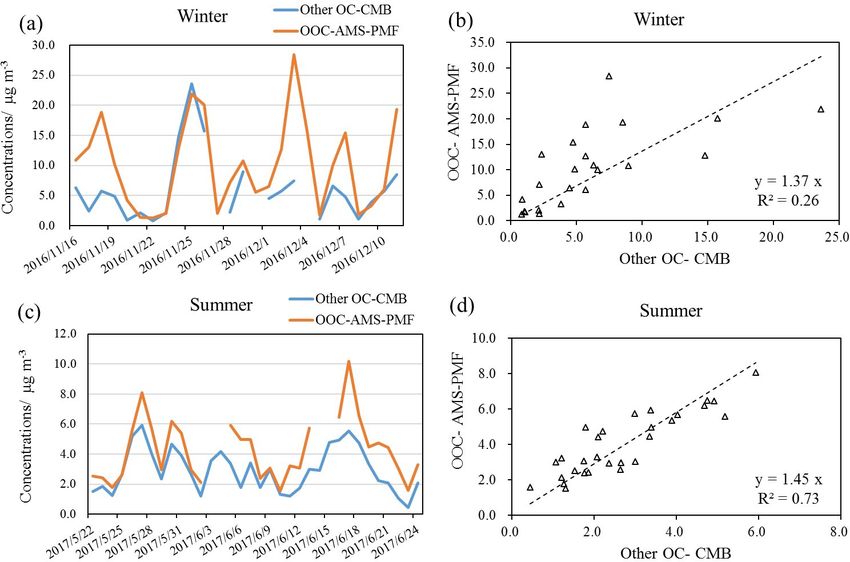
J. Xu et al.: Source apportionment of fine OC in urban Beijing                                                                        7323

Figure 1. Locations of the sampling sites in Beijing (IAP – urban site: Institute of Atmospheric Physics of the Chinese Academy of Sciences;
Pinggu – rural site) (source: © Google Maps).

et al., 2019). The sampling site (Fig. 1) is located in the             with the pump turned off during the sampling campaign.
middle between the North 3rd Ring Road and North 4th                    Before and after sampling, all filters were put in a balance
Ring Road and approximately 200 m from a major highway.                 room and equilibrated at a constant temperature and rela-
Hence, it is subject to many local sources, such as traffic,            tive humidity (RH) for 24 h prior to any gravimetric mea-
cooking, etc. The location of a rural site in Beijing–Pinggu            surements, which were 22 ◦ C and 30 % RH for summer sam-
during the APHH-China campaigns is also shown in Fig. 1.                ples and 21 ◦ C and 33 % RH for winter samples. PM2.5 mass
The rural site in Xibaidian village in Pinggu is about 60 km            was determined through the weighing of PTFE filters using a
away from IAP and 4 km northwest of Pinggu town center.                 microbalance (Sartorius model MC5; precision: 1 µg). After
It is surrounded by trees and farmland with several similar             that, filters were wrapped separately with aluminum foil and
small villages nearby. A provincial highway is approximately            stored at under −20 ◦ C in darkness until analysis. The large
500 m away on its east side running north–south. This site is           quartz filters were analyzed for OC, EC, organic compounds,
far from industrial sources and located in a residential area.          and ion species, while small PTFE filters were used for the
Other information regarding the sampling site is described              determination of PM2.5 mass and metals. Online PM2.5 con-
elsewhere (Shi et al., 2019).                                           centrations were determined by the TEOM FDMS 1405-DF
   PM2.5 samples were collected on pre-baked (450 ◦ C for               instrument at IAP with filter equilibrating and weighing con-
6 h) large quartz filters (Pallflex, 8 in × 10 in) by high vol-         ditions comparable with the United States Federal Reference
ume air sampler (Tisch, USA) at a flow rate of 1.1 m3 min−1 .           Method (RH: 30 %–40 %; temperature: 20–23 ◦ C) (Le et al.,
A medium volume air sampler (Thermo Scientific Partisol                 2020; U.S.EPA, 2016).
2025i) was also deployed at the same location to collect
PM2.5 samples simultaneously on 47 mm PTFE filters at a
flow rate of 15.0 L min−1 . Field blanks were also collected

https://doi.org/10.5194/acp-21-7321-2021                                                   Atmos. Chem. Phys., 21, 7321–7341, 2021

7324                                                        J. Xu et al.: Source apportionment of fine OC in urban Beijing

2.2     Chemical analysis                                        was obtained by spiking standards to pre-baked blank quartz
                                                                 filters followed by the same extraction and derivatization
2.2.1    OC and EC                                               procedures. Field blank filters were analyzed the same way
                                                                 as samples for quality assurance, but no target compounds
A 1.5 cm2 punch from each large quartz filter sample was         were detected.
taken for organic carbon (OC) and elemental carbon (EC)
measurements by a thermal-optical carbon analyzer (model         2.2.3    Inorganic components
RT-4, Sunset Laboratory Inc., USA) based on the EU-
SAAR2 (European Supersites for Atmospheric Aerosol Re-           Half of the PTFE filter was extracted with 10 mL ultrapure
search) transmittance protocol (Cavalli et al., 2010; L.-W. A.   water for the analysis of inorganic ions. Major inorganic ions
                                                                                                                 2−
Chen et al., 2015). Replicate analyses of OC and EC were         including Na+ , K+ , NH+       −      −
                                                                                          4 , Cl , NO3 , and SO4 were deter-
conducted once every 10 samples. The uncertainties from          mined by using an ion chromatograph (IC; Dionex, Sunny-
duplicate analyses of filters were < 10 %. All sample re-        vale, CA, USA), and the detection limits (DLs) of them were
sults were corrected by the values obtained from field blanks,   0.032, 0.010, 0.011, 0.076, 0.138, 0.240, and 0.142 µg m−3 ,
which were 0.40 and 0.01 µg m−3 for OC and EC, respec-           respectively. The analytical uncertainty was less than 5 %
tively. Details of the OC/EC measurement method can be           for all inorganic ions. An intercomparison study showed that
found elsewhere (Paraskevopoulou et al., 2014). The instru-      our IC analysis of the abovementioned ions agreed well with
mental limits of detection of OC and EC in this study were       those of the other laboratories (Xu et al., 2020).
estimated to be 0.03 and 0.05 µg m−3 , respectively.                For winter samples, crustal elements including Al (DLs
                                                                 in µg m−3 ; 0.221), Si (0.040), Ca (0.034), Ti (0.003), and Fe
2.2.2    Organic compounds                                       (0.044) were determined by X-ray fluorescence spectrometry
                                                                 (XRF), and trace metals including V, Cr, Co, Mn, Ni, Cu, Zn,
Organic tracers, including 11 n-alkanes (C24 -C34 ),             As, Sr, Cd, Sb, Ba, and Pb were analyzed by inductively cou-
2 hopanes (17a(H)-22,29,30-trisnorhopane, 17b(H),21a(H)-         pled plasma mass spectrometry (ICP-MS) after the extraction
norhopane), 17 PAHs (retene, phenanthrene, an-                   of one-half of the PTFE filter by diluted acid mixture (HNO3
thracene,     fluoranthene,    pyrene,     benz(a)anthracene,    and HCl) with a detection limit of 1.32, 0.25, 0.04, 0.06, 2.05,
chrysene, benzo(b)fluoranthene, benzo(k)fluoranthene,            1.25, 1.22, 1.74, 0.02, 0.03, 0.11, 0.06, and 0.04 ng m−3 , re-
benzo(e)pyrene, benzo(a)pyrene, perylene, indeno(1,2,3-          spectively. For summer samples, apart from Al, Si, Ca, Ti,
cd)pyrene, dibenz(a,h)anthracene, benzo(ghi)perylene,            and Fe as mentioned above, V, Cr, Co, Mn, Ni, Cu, Zn, As, Sr,
coronene, picene), 3 anhydrosugars (levoglucosan, man-           Cd, Sb, Ba, and Pb were also analyzed by XRF with the DLs
nosan, galactosan), 2 fatty acids (palmitic acid, stearic        of 0.004, 0.002, 0.0005, 0.001, 0.005, 0.026, 0.002, 0.0004,
acid), and cholesterol, in the PM2.5 samples were deter-         0.001, 0.013, 0.077, 0.0004, and 0.003 µg m−3 , respectively.
mined in this study. A total of 9 cm2 of the large quartz        More details are given in Srivastava et al. (2021). Mass con-
filters was extracted three times with dichloromethane and       centrations of all inorganic ions and elements in this study
methanol (HPLC grade; v/v: 2 : 1) under ultrasonication          were corrected for the field blank values, and the methods
for 10 min. The extracts were then filtered and concentrated     were quality assured with standard reference materials.
using a rotary evaporator under vacuum and blown down
                                                                 2.3     Chemical mass closure (CMC) method
to dryness with pure nitrogen gas. A total of 50 µL of
N,O-bis-(trimethylsilyl)trifluoroacetamide (BSTFA) with          A chemical mass closure analysis was carried out, which in-
1 % trimethylsilyl (TMS) chloride and 10 µL of pyridine          cludes secondary inorganic ions (sulfate, nitrate, ammonium;
was then added to the extracts, which were left reacting         SNA), sodium, potassium, and chloride salts, geological min-
at 70 ◦ C for 3 h to derivatize -COOH to TMS esters and          erals, trace elements, organic matter (OM), EC, and bound
-OH to TMS ethers. After cooling to room temperature, the        water in reconstructed PM2.5 . Geological minerals were cal-
derivatives were diluted with 140 µL of internal standards       culated by applying Eq. (1) (Chow et al., 2015).
(C13 n-alkane, 1.43 ng µL−1 ) in n-hexane prior to GC-MS
(gas chromatography mass spectrometry) analysis. The             Geological minerals = 2.2Al + 2.49Si + 1.63Ca
final solutions were analyzed by a gas chromatography                                    + 1.94Ti + 2.42Fe                   (1)
mass spectrometry system (GC-MS; Agilent 7890A GC
plus 5975C mass-selective detector) fitted with a DB-5MS            Trace elements were the sum of all analyzed elements
column (30 m × 0.25 mm × 0.25 µm). The GC temperature            excluding Al, Si, Ca, Ti, and Fe. The average OM/OC ra-
program and MS detection details were reported in Li             tios of organic aerosols (OAs) from AMS elemental analysis
et al. (2018). Individual compounds were identified through      were applied to calculate OM, which were 1.75 ± 0.16 and
the comparison of mass spectra with those of authentic           2.00 ± 0.19 in winter and summer, respectively. Based on the
standards or literature data (Fu et al., 2016). Recoveries for   concentrations of inorganic ions and gas-phase NH3 , particle
these compounds were in a range of 70 %–100 %, which             bound water was calculated with the ISORROPIA II model

Atmos. Chem. Phys., 21, 7321–7341, 2021                                            https://doi.org/10.5194/acp-21-7321-2021
J. Xu et al.: Source apportionment of fine OC in urban Beijing                                                                7325

(available at http://isorropia.eas.gatech.edu, last access: July     sis of organic aerosol (OA) mass spectra, can be found else-
2020) in forward mode and thermodynamically metastable               where (W. Xu et al., 2019). The source apportionment of or-
phase state (Fountoukis and Nenes, 2007). Two sets of cal-           ganics in NR-PM1 was carried out by applying PMF to the
culations were done for online and offline data, differing in        high-resolution mass spectra of OA, while that of fine OC in
the temperature and relative humidity as specified above.            this study was conducted by applying source profiles along
                                                                     with an offline chemical speciation dataset. The procedures
2.4   Chemical mass balance (CMB) model                              of the pretreatment of spectral data and error matrices can
                                                                     be found elsewhere (Ulbrich et al., 2009). It is noted that the
The chemical mass balance model (US EPA CMB8.2)                      data were missing during the period 9–15 November 2016
was applied in this study to apportion the sources of OC             due to the malfunction of the AMS.
by utilizing a linear least squares solution. Uncertainties
in both source profiles and ambient measurements were
taken into consideration in this model. The source profiles
applied here were from local studies in China to better              3     Results and discussion
represent the source characteristics, including straw burn-
ing (wheat, corn, rice straw burning) (Y.-X. Zhang et al.,           3.1    Characteristics of PM2.5 and carbonaceous
2007), wood burning (Wang et al., 2009), gasoline and                       compounds
diesel vehicles (including motorcycles, light- and heavy-
duty gasoline and diesel vehicles) (Cai et al., 2017), indus-        Mean concentrations of PM2.5 , OC, EC, and organic tracers
trial and residential coal combustion (including anthracite,         during wintertime (9 November to 11 December 2016) and
sub-bituminite, bituminite, and brown coal) (Zhang et al.,           summertime (22 May to 24 June 2017) at the IAP site are
2008), and cooking (Zhao et al., 2015), except vegeta-               summarized in Table 1 and Fig. S1 in the Supplement. The
tive detritus (Rogge et al., 1993; Wang et al., 2009). The           average PM2.5 concentration was 94.8 ± 64.4 µg m−3 during
source profiles with EC and organic tracers used in the              the whole winter sampling campaign. The winter sampling
CMB model were provided in Table S1 of Wu et al.                     period was divided into haze (daily PM2.5 > 75 µg m−3 ) and
(2020). The selected fitting species were EC, levoglucosan,          non-haze days (< 75 µg m−3 ), based on the National Ambi-
palmitic acid, stearic acid, fluoranthene, phenanthrene,             ent Air Quality Standard Grade II of the limit for 24 h av-
retene, benz(a)anthracene, chrysene, benzo(b)fluoranthene,           erage PM2.5 concentration. The differentiation between haze
benzo(k)fluoranthene, benzo[ghi]perylene, picene, 17a(H)-            and non-haze days enabled us to study the major sources con-
22,29,30-trisnorhopane, 17b(H),21a(H)-norhopane, and n-              tributing to the haze formation. The average daily PM2.5 was
alkanes (C24–C33), the concentrations of which are provided          136.7 ± 49.8 and 36.7 ± 23.5 µg m−3 on haze and non-haze
in Table 1. The essential criteria in this model were met to         days, respectively. Daily PM2.5 in the summer sampling pe-
ensure reliable fitting results. For instance, in all samples, R 2   riod was 30.2 ± 14.8 µg m−3 , comparable with that on winter
values were > 0.80 (mostly > 0.9), Chi2 values were < 2,             non-haze days.
Tstat values were mostly greater than 2 except the source of            OC concentrations ranged between 3.9–48.8 µg m−3
vegetative detritus, and C/M ratios (ratio of calculated to          (mean: 21.5 µg m−3 ) and 1.8–12.7 µg m−3 (mean:
measured concentration) for all fitting species were in range        6.4 µg m−3 ) during winter and summer, respectively.
of 0.8–1.2 in this study.                                            They are comparable with the OC concentrations in win-
                                                                     ter (23.7 µg m−3 ) and summer (3.78 µg m−3 ) in Tianjin,
2.5   Positive matrix factorization analysis of data                 China, during an almost simultaneous sampling period (Fan
      obtained from aerosol mass spectrometer                        et al., 2020) but much lower than the OC concentration
      (AMS-PMF)                                                      (17.1 µg m−3 ) in summer 2007 in Beijing (Yang et al.,
                                                                     2016). The average OC concentration during haze days
An Aerodyne AMS with a PM1 aerodynamic lens was de-                  (29.4 ± 9.2 µg m−3 ) was approximately 3 times that of
ployed on the roof of the neighboring building, the tower            non-haze days (10.7 ± 6.2 µg m−3 ) during winter. The aver-
branch of IAP, for real-time measurements of non-refractory          age EC concentration during winter was 3.5 ± 2.0 µg m−3 ;
(NR) chemical species from 16 November to 11 Decem-                  its concentration was 4.6 ± 1.3 µg m−3 on haze days,
ber 2016 and 22 May to 24 June 2017. The detailed infor-             approximately 2.4 times that on winter non-haze days
mation of the sampling sites is given elsewhere (W. Xu et al.,       (1.9 ± 1.6 µg m−3 ), and 5 times that (0.9 ± 0.4 µg m−3 )
2019). The submicron particles were dried and sampled into           during the summer sampling period. The OC and EC
the AMS at a flow of ∼ 0.1 L min−1 . NR-PM1 can be quickly           concentrations in this study were comparable with the OC
vaporized by the 600 ◦ C tungsten vaporizer, and then the NR-        (27.9 ± 23.4 µg m−3 ) and EC (6.6 ± 5.1 µg m−3 ) concen-
                                                2−
PM1 species including organics, Cl− , NO− 3 , SO4 , and NH4
                                                            +
                                                                     trations in winter Beijing in 2016 (Qi et al., 2018) but
were measured by AMS in mass sensitive V mode (Sun et al.,           much lower than those in an urban area of Beijing during
2020). Details of AMS data analysis, including the analy-            winter (OC and EC: 36.7 ± 19.4 and 15.2 ± 11.1 µg m−3 )

https://doi.org/10.5194/acp-21-7321-2021                                              Atmos. Chem. Phys., 21, 7321–7341, 2021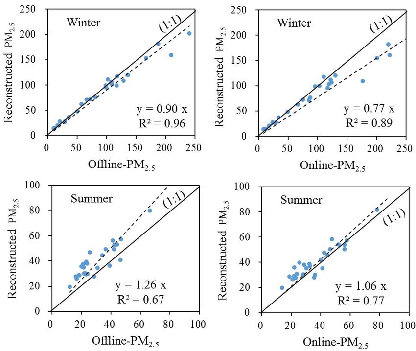
7326                                                                                J. Xu et al.: Source apportionment of fine OC in urban Beijing

Table 1. Summary of measured concentrations at IAP site in winter and summer.

   Compoundsa                                                   Winter                                                    Winter (n = 31)                Summer (n = 34)
   (ng m−3 )
                                                 Hazed (n = 18)                 Non-hazee (n = 13)
   PM2.5 (µg m−3 )                136.7 ± 49.8 (80.5–239.9)b                 36.7 ± 23.5 (10.3–72)            94.8 ± 64.4 (10.3–239.9)           30.2 ± 14.8 (12.2–78.8)
   OC (µg m−3 )                        29.4 ± 9.2 (13.7–48.8)                 10.7 ± 6.2 (3.9–21.5)              21.5 ± 12.3 (3.9–48.8)             6.4 ± 2.3 (1.8–12.7)
   EC (µg m−3 )                            4.6 ± 1.3 (1.6–6.6)                  1.9 ± 1.6 (0.3–5.2)                 3.5 ± 2.0 (0.3–6.6)               0.9 ± 0.4 (0.2–1.7)
   SOCc (µg m−3 )                       10.3 ± 5.7 (2.9–24.6)                   2.9 ± 1.4 (0.0–5.5)                7.2 ± 5.7 (0.0–24.6)               2.3 ± 1.4 (0.0–6.0)
   Levoglucosan                   348.2 ± 148.0 (83.1–512.5)           195.0 ± 163.7 (19.1–539.5)           278.5 ± 171.4 (19.1–539.5)           26.1 ± 28.3 (2.9–172.2)
   Palmitic acid                 376.2 ± 234.9 (44.5–1089.6)            278 ± 280.6 (33.8–1137.2)            335 ± 255.3 (33.8–1137.2)              25.2 ± 11.9 (9.4–68)
   Stearic acid                    207.1 ± 181.4 (23–846.7)            163.6 ± 228.1 (17.3–903.2)           188.8 ± 199.8 (17.3–903.2)             16.0 ± 7.2 (5.6–36.4)
   Phenanthrene                            8.6 ± 6.1 (1.8–19)                    5.6 ± 6.1 (1–24.8)                   7.3 ± 6.2 (1–24.8)                0.7 ± 0.7 (0–3.8)
   Fluoranthene                        25.1 ± 19.6 (4.2–76.2)               16.1 ± 21.3 (4.2–84.3)               21.3 ± 20.5 (4.2–84.3)                 0.4 ± 0.2 (0–0.9)
   Retene                                 16 ± 14.9 (2–52.2)                11.1 ± 12.1 (0.5–45.5)               13.9 ± 13.8 (0.5–52.2)                     0 ± 0 (0–0.1)
   Benz(a)anthracene                   21.5 ± 16.5 (0.3–62.7)                 10.8 ± 9.3 (1.4–30.5)                17 ± 14.8 (0.3–62.7)                 0.2 ± 0.1 (0–0.5)
   Chrysene                            22.6 ± 14.1 (3.7–47.3)               13.6 ± 15.6 (0.1–59.5)               18.8 ± 15.2 (0.1–59.5)                 0.2 ± 0.1 (0–0.3)
   Benzo(b)fluoranthene                  52.6 ± 29 (10.7–98)                 28.1 ± 31 (2.4–113.6)             42.3 ± 31.8 (2.4–113.6)                    0.7 ± 0.5 (0–2)
   Benzo(k)fluoranthene                     12.2 ± 8 (0–25.3)                    6.7 ± 6.8 (0–23.7)                   9.9 ± 7.9 (0–25.3)                0.2 ± 0.1 (0–0.4)
   Picene                                    0.8 ± 0.8 (0–2.6)                    0.3 ± 0.5 (0–1.3)                    0.6 ± 0.7 (0–2.6)                      0 ± 0 (0–0)
   Benzo(ghi)perylene                      7.0 ± 4.7 (0–13.6)                    4.0 ± 4.1 (0–14.0)                   5.6 ± 4.6 (0–14.0)                  0 ± 0.1 (0–0.3)
   17a(H)-22,29,30-                        2.7 ± 1.6 (0.6–6.7)                    1.6 ± 1.5 (0.3–6)                  2.2 ± 1.6 (0.3–6.7)                  0 ± 0.1 (0–0.4)
   trisnorhopane
   17b(H),21a(H)-                            3.1 ± 1.6 (0.9–6.6)                  1.8 ± 1.8 (0.3–7.3)                  2.6 ± 1.8 (0.3–7.3)                    0 ± 0 (0–0.2)
   norhopane
   C24                                  26.3 ± 15.3 (7.8–55.5)                 18 ± 19.2 (2.1–71.2)               22.5 ± 17.4 (2.1–71.2)               1.4 ± 0.6 (0.5–3.3)
   C25                                    28.2 ± 15.6 (8.5–59)               19.5 ± 20.5 (2.3–76.2)               24.2 ± 18.3 (2.3–76.2)               2.9 ± 1.5 (0.5–6.5)
   C26                                  18.9 ± 10.2 (5.8–40.2)                 13 ± 13.1 (1.8–48.2)               16.2 ± 11.8 (1.8–48.2)               1.6 ± 0.7 (0.3–4.3)
   C27                                   20.4 ± 9.2 (6.1–37.1)               13.8 ± 12.5 (2.2–43.5)               17.4 ± 11.2 (2.2–43.5)                4.4 ± 2 (0.6–11.7)
   C28                                   10.6 ± 4.8 (3.2–19.2)                 6.9 ± 5.7 (1.5–19.3)                 8.9 ± 5.5 (1.5–19.3)               1.4 ± 0.6 (0.3–2.9)
   C29                                  22.3 ± 10.1 (5.9–39.7)                   14.3 ± 12.6 (3–39)                18.7 ± 11.9 (3–39.7)               5.2 ± 3.3 (0.4–20.7)
   C30                                    6.8 ± 2.9 (2.2–11.4)                     4.5 ± 3.1 (1–9.7)                  5.7 ± 3.2 (1–11.4)                   1 ± 0.4 (0.2–2)
   C31                                   11.6 ± 4.2 (3.5–17.7)                 7.7 ± 5.8 (1.2–18.7)                 9.8 ± 5.3 (1.2–18.7)                4.3 ± 3.2 (0.4–20)
   C32                                      6.1 ± 2.6 (1.7–9.3)                 3.9 ± 2.6 (0.7–8.2)                  5.1 ± 2.8 (0.7–9.3)               0.9 ± 0.4 (0.2–1.7)
   C33                                     5.8 ± 2.7 (1.7–11.5)                  3.9 ± 3.1 (0.9–9.6)                  4.9 ± 3 (0.9–11.5)               1.8 ± 1.1 (0.1–6.3)
   C34                                        2.1 ± 2.1 (0–5.5)                      1.2 ± 1.4 (0–4)                   1.7 ± 1.8 (0–5.5)                 0.3 ± 0.3 (0–0.9)
  a The unit is nanograms per cubic meter (ng m−3 ) for all organic compounds and microgram per cubic meter (µg m−3 ) for PM , OC, EC, and SOC; b mean ± SD (min–max); c SOC
                                                                                                                            2.5
  concentration was calculated by EC-tracer method; d haze days: PM2.5 ≥ 75 µg m−3 ; e non-haze days: PM2.5 < 75 µg m−3 .

Figure 2. Chemical components of reconstructed PM2.5 (offline) applying mass closure method.

Atmos. Chem. Phys., 21, 7321–7341, 2021                                                                              https://doi.org/10.5194/acp-21-7321-2021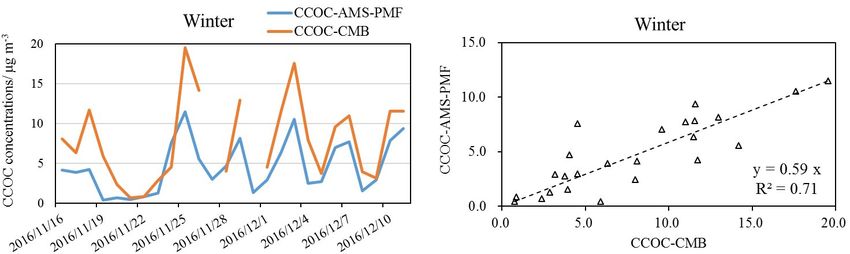
J. Xu et al.: Source apportionment of fine OC in urban Beijing                                                           7327

and summer (10.7 ± 3.6 and 5.7 ± 2.9 µg m−3 ) in 2002 (Dan       structed PM2.5 , followed by the secondary inorganic ions
                                                                            2−
et al., 2004).                                                   (NH+               −
                                                                      4 , SO4 , NO3 ) (35.0 %). In summer, in contrast, sec-
   On average, OC and EC concentrations in winter were 3.3       ondary inorganic salts represented 45.2 % of PM2.5 mass,
and 3.9 times those in summer. Additionally, OC and EC           followed by carbonaceous components (35.2 %). Bound wa-
were well-correlated in this study, with R 2 values of 0.85      ter contributed 4.6 % and 7.2 % of PM2.5 during the winter
and 0.63 during winter and summer, respectively, suggesting      and summer, respectively. All other components combined
similar paths of OC and EC dispersion and dilution and/or        accounted for 13.2 % and 12.4 % of PM2.5 during the winter
similar sources of carbonaceous aerosols, especially in win-     and summer campaigns, respectively.
ter. Less correlated OC and EC in summer could be a result
of SOC formation. SOC in this study was estimated and is         3.3     Source apportionment of fine OC in urban Beijing
discussed in Sect. 3.3.7.                                                applying a CMB model

3.2   Chemical mass closure (CMC)                                The CMB model resolved seven primary sources of OC
                                                                 in winter and summer, including vegetative detritus, straw
The composition of PM2.5 applying the chemical mass clo-         and wood burning (biomass burning, BB), gasoline vehicles,
sure method is plotted in Fig. 2 and summarized in Ta-           diesel vehicles, industrial coal combustion (industrial CC),
ble S1 in the Supplement. Because the gravimetrically mea-       residential coal combustion (residential CC), and cooking. It
sured mass (offline PM2.5 ) differs slightly from online PM2.5   explained an average of 75.7 % (45.3 %–91.3 %) and 56.1 %
(Fig. S2 in the Supplement), the regression analysis re-         (34.3 %–76.3 %) of fine OC in winter and summer, respec-
sults between mass reconstructed using mass closure (recon-      tively. The averaged CMB source apportionment results in
structed PM2.5 ) and both measured PM2.5 concentrations (of-     winter and summer are presented in Table 2. Daily source
fline PM2.5 and online PM2.5 ) were investigated and plotted     contribution estimates to fine OC and the relative abundance
in Fig. 3.                                                       of different sources contributions to OC in winter and sum-
   As shown in Fig. 3, measured offline and online PM2.5         mer are shown in Fig. 4.
concentrations were moderately well-correlated with the re-         During the winter campaign, coal combustion (industrial
constructed PM2.5 with slopes of 0.77 ∼ 1.26 and R 2 of          and residential CC, 7.5 µg m−3 , 35.0 % of OC) was the
0.67 ∼ 0.96. In winter, the regression results were good be-     most significant contributor to OC, followed by other OC
tween reconstructed PM2.5 and offline PM2.5 . For online         (5.3 µg m−3 , 24.8 %), biomass (3.8 µg m−3 , 17.6 %), traffic
PM2.5 , it was much higher than the reconstructed PM2.5          (gasoline and diesel vehicles, 2.6 µg m−3 , 11.9 %), cooking
when the mass was over 170 µg m−3 . After excluding the out-     (2.2 µg m−3 , 10.3 %), and vegetative detritus (0.09 µg m−3 ,
liers (two outliers of offline PM2.5 > 200 µg m−3 and four       0.4 %). On winter haze days, industrial coal combustion,
outliers of online PM2.5 > 170 µg m−3 ), the regression re-      cooking, and other OC were significantly higher (nearly
sults improved with both slopes and R 2 approaching unity        tripled) compared to non-haze days. During the summer
(Fig. S3 in the Supplement). This could indicate some un-        campaign, other OC (2.9 µg m−3 , 45.6 %) was the most sig-
certainties in offline and/or online PM2.5 measurements for      nificant contributor to OC, followed by coal combustion
heavily polluted samples, or the applied OM/OC ratio in          (2.0 µg m−3 , 31.1 %), cooking (0.7 µg m−3 , 10.3 %), traffic
winter was not suitable for converting OC to OM in heavily       (0.4 µg m−3 , 6.1 %), biomass burning (0.3 µg m−3 , 5.3 %),
polluted samples. During the summer campaign, the slope          and vegetative detritus (0.1 µg m−3 , 1.7 %).
of the reconstructed PM2.5 and online PM2.5 was close to 1,
but that of reconstructed PM2.5 and offline PM2.5 was 1.26.      3.3.1    Industrial and residential coal combustion
This could be due to the loss of semi-volatile compounds
from PTFE filters or the positive artifacts of quartz filters    In China, a large amount of coal is used in thermal power
for chemical analyses which can absorb more organics than        plants, industries, and urban and rural houses in northern
PTFE filters that are used for PM weighing. To avoid loss        China, especially during the heating period (mid-November
of semi-volatiles, all collected samples were stored in cold     to mid-March) (Huang et al., 2017; Yu et al., 2019), but urban
conditions, including during shipment. The data points were      household coal use experienced a remarkable drop of 58 %
more scattered in summer, which could result from the large      during 2005–2015, which is much higher than that of rural
difference in OM–OC relationships from day to day. The re-       household coal use (5 % of decrease) (Zhao et al., 2018).
constructed inorganics (reconstructed PM2.5 excluding OM)        In this study, coal combustion is the single largest source
correlated well with offline PM2.5 , but OM did not (Fig. S4     that contributed to primary OC in both winter and sum-
in the Supplement). Hence, the discrepancies between recon-      mer. In addition, industrial CC was a more significant source
structed PM2.5 and offline and online PM2.5 in summer may        of OC than residential CC in urban Beijing. On average,
be mainly attributable to variable OM/OC ratios.                 coal-combustion-related OC (CCOC) was 7.5 ± 5.0 µg m−3
   During the winter campaign, the carbonaceous compo-           (34.5 ± 9.8 % of OC) in winter, which was more than 3 times
nents (OM and EC) accounted for 47.2 % of total recon-           that in summer – 2.0 ± 0.8 µg m−3 (32.3 ± 10.2 % of OC),

https://doi.org/10.5194/acp-21-7321-2021                                          Atmos. Chem. Phys., 21, 7321–7341, 2021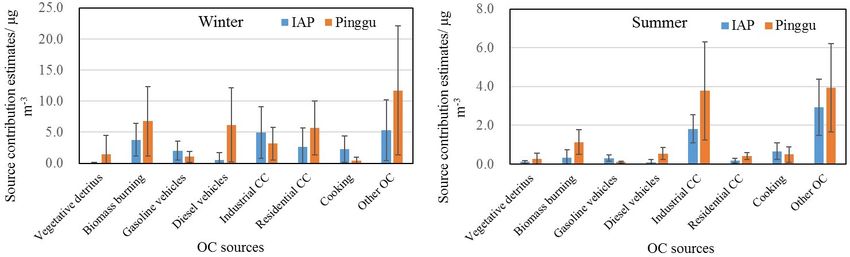
7328                                                                             J. Xu et al.: Source apportionment of fine OC in urban Beijing

Figure 3. Regression results between reconstructed PM2.5 and offline and online PM2.5 by chemical mass closure method.

Table 2. Source contribution estimates (SCEs; µg m−3 ) for fine OC in urban Beijing during winter and summer from the CMB model.

             Sources                                                          Winter                          Winter (n = 31)           Summer (n = 34)
                                                          Haze (n = 18)          Non-haze (n = 13)
             Vegetative detritus                              0.11 ± 0.08                  0.07 ± 0.08              0.09 ± 0.08                 0.11 ± 0.08
             Biomass burning                                  4.80 ± 2.23                  2.38 ± 2.57              3.78 ± 2.64                 0.34 ± 0.39
             Gasoline vehicles                                2.35 ± 1.27                  1.59 ± 1.85              2.03 ± 1.56                 0.31 ± 0.16
             Diesel vehicles                                  0.83 ± 1.43                  0.14 ± 0.33              0.54 ± 1.15                 0.08 ± 0.16
             Industrial coal combustion                       7.09 ± 4.17                  1.95 ± 1.36              4.94 ± 4.15                 1.82 ± 0.72
             Residential coal combustion                      3.64 ± 3.72                  1.16 ± 0.96              2.60 ± 3.12                 0.18 ± 0.11
             Cooking                                          3.23 ± 2.30                  0.85 ± 0.52              2.23 ± 2.13                 0.66 ± 0.43
             Other OCa                                          7.4 ± 5.6                     2.5 ± 1.4               5.3 ± 4.9                   2.9 ± 1.5
             Calculated OCb                                    22.0 ± 6.5                     8.2 ± 5.3              16.2 ± 9.1                   3.5 ± 1.2
             Measured OC                                       29.4 ± 9.2                   10.7 ± 6.2              21.5 ± 12.3                   6.4 ± 2.3
           a Other OC is calculated by subtracting calculated OC from measured OC. b Calculated OC is the sum of OC from all seven primary sources:
           vegetative detritus, biomass burning, gasoline vehicles, diesel vehicles, industrial coal combustion, residential coal combustion, and cooking.

but the percentage contribution is similar. A similar seasonal                           an important contribution to haze formation from industrial
trend was also found in other studies in Beijing (Zheng et al.,                          CC.
2005; Wang et al., 2009), but the relative contribution of coal                             Coal combustion is also a major source for particulate
combustion was much lower than in this study. Industrial-                                chloride (Chen et al., 2014). Because Beijing is an inland
CC-derived OC was 4.94 ± 4.15 and 1.82 ± 0.72 µg m−3                                     city, the contribution of marine aerosols to particulate Cl−
in winter and summer, respectively. Residential-CC-derived                               is considered minor, which is also supported by the higher
OC was 2.60 ± 3.12 and 0.18 ± 0.11 µg m−3 in winter and                                  Cl− /Na+ mass ratios in winter (10.1 ± 4.8) and summer
summer, respectively. Residential CC was much higher in                                  (2.7 ± 1.8) than seawater (1.81), indicative of significant con-
winter compared to that in summer. On haze days, industrial-                             tributions from anthropogenic sources (Bondy et al., 2017).
CC- and residential-CC-derived OC concentrations were 3.6                                Yang et al. (2018) also reported that the contribution of
and 3.1 times that on non-haze days, respectively, indicating                            sea-salt aerosol to fine particulate chloride was negligible

Atmos. Chem. Phys., 21, 7321–7341, 2021                                                                           https://doi.org/10.5194/acp-21-7321-2021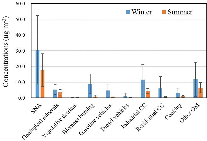
J. Xu et al.: Source apportionment of fine OC in urban Beijing                                                                 7329

Figure 4. Daily source contribution estimates for fine OC in (a) winter and (c) summer and their relative abundance in winter (b) and
summer (d).

Figure 5. Time series of OC from coal combustion (OC-CC) and Cl− in winter and summer in Beijing.

in Chinese inland areas even during summer. Hence, Cl−               ing biomass burning. In addition, due to the semi-volatility
in this study was mainly from anthropogenic sources. The             of ammonium chloride, it is liable to evaporate in summer
time series of OC from coal combustion (OC-CC) and Cl−               (Pio and Harrison, 1987). A similar phenomenon has been
during winter and summer in Beijing are shown in Fig. 5.             observed in Delhi (Pant et al., 2015).
OC-CC and Cl− exhibited similar trends in both seasons.
The correlation coefficient (R 2 ) between OC-CC and Cl−             3.3.2   Biomass burning
during winter was 0.62, which could be attributed to en-
hanced coal combustion activities in this season. No signifi-        Biomass burning (BB), including straw and wood burn-
cant correlation between the two was found during the sum-           ing, is an important source of atmospheric fine OC, which
mer campaign, indicating that the abundance of Cl− in sum-           ranked as the second highest primary source of OC after
mer was more influenced by other sources, probably includ-           industrial coal combustion during the winter campaign and
                                                                     third highest during the summer campaign after industrial

https://doi.org/10.5194/acp-21-7321-2021                                              Atmos. Chem. Phys., 21, 7321–7341, 2021
7330 J. Xu et al.: Source apportionment of fine OC in urban Beijing
CC and cooking. As shown in Fig. 4, the relative abun- summer, respectively. The summer result was comparable
dance of BB-derived OC during the winter campaign is much with the vehicular emission contribution to PM2.5 (2.1 %) in
higher than the summer campaign. BB-derived OC from summer in Beijing but higher than that in winter (1.5 %) in
the CMB results was 3.78 ± 2.64 and 0.34 ± 0.39 µg m−3 in Beijing estimated by using a PMF model (Yu et al., 2019).
winter and summer, contributing 17.6 % and 5.3 % of OC Gasoline vehicles dominated the traffic emissions; gasoline-
in these two seasons, respectively. These results are lower vehicle-derived OC was 2.03 ± 1.56 and 0.31 ± 0.16 µg m−3
than those in 2005–2007 in Beijing when BB accounted for in winter and summer, respectively, which are approxi-
26 % and 11 % of OC in winter and summer, respectively mately 4 times that in winter (0.54 ± 1.15 µg m−3 ) and
(Wang et al., 2009). The BB-derived OC on winter haze days summer (0.08 ± 0.16 µg m−3 ) attributed to diesel vehicles.
(4.80 ± 2.23 µg m−3 ) was approximately double that of non- On haze days, gasoline- and diesel-derived OC concentra-
haze days (2.38 ± 2.57 µg m−3 ), accounting for 16.3 % and tions were 2.35 ± 1.27 and 0.83 ± 1.43 µg m−3 , respectively,
22.2 % of OC on haze and non-haze days, respectively. much higher than gasoline- (1.59 ± 1.85 µg m−3 ) and diesel-
Levoglucosan is widely used as a key tracer for biomass derived (0.14 ± 0.33 µg m−3 ) OC on non-haze days. Even
burning emissions (Bhattarai et al., 2019; Cheng et al., 2013; though diesel vehicles played a less important role in OC
J. Xu et al., 2019). Based on a levoglucosan to OC ratio of emissions, diesel-derived OC on haze days increased by
8.2 % (X.-Y. Zhang et al., 2007; Fan et al., 2020), the BB- around 6 times above that of non-haze days, and such an in-
derived OC was 3.40 ± 2.09 µg m−3 and 0.32 ± 0.35 µg m−3 crease was much higher than for gasoline, suggesting a po-
during the winter and summer campaigns, respectively. tentially important role of diesel emissions in haze formation.
These results are comparable to BB-derived OC from the
CMB model in this study. The estimated BB-derived OC 3.3.4 Cooking
concentrations are also comparable with the BB-derived OC
during the same sampling periods in Tianjin (Fan et al., Cooking is expected to be an important contributor of fine
2020) but higher than those at IAP in 2013/14 (Kang et al., OC in densely populated Beijing, which has a population
2018). Both of the studies applied the levoglucosan/OC ra- of over 21 million. The cooking source profile was se-
tio method to estimate the BB-derived OC, although the ac- lected from a study which was carried out in the urban
tual ratio in Beijing air may be very different from 8.2 %. area of another Chinese megacity, Guangzhou, which in-
The heavily elevated OC concentration in winter compared cludes fatty acids, sterols, monosaccharide anhydrides, alka-
to summer could be a result of increased biomass burning nes, and PAHs in particles from Chinese residential cooking
activities for house heating and cooking in Beijing in addi- (Zhao et al., 2015). The resulting cooking-related OC con-
tion to the unfavorable dispersion conditions under stagnant centrations were 2.23 ± 2.13 µg m−3 and 0.66 ± 0.43 µg m−3
weather conditions in the winter. in winter and summer, respectively, and both accounted for
In summer, the total OC concentration was highest on about 10 % of total OC. Cooking OC was 3.23 ± 2.30 µg m−3
17 June. The sudden rise in OC on this day was attributed on winter haze days, around 4 times higher than that on non-
to the enhanced biomass burning activities, which led to the haze days (0.85 ± 0.52 µg m−3 ).
highest level of BB-derived OC and highest biomass burning
3.3.5 Vegetative detritus
organic carbon (BBOC) to OC abundance. The levoglucosan
concentration on this day was also the highest in summer, Vegetative detritus made a minor contribution to fine parti-
which reached 172 ng m−3 . cle mass. Its concentration was 0.09 ± 0.08 µg m−3 (0.4 %)
and 0.11 ± 0.08 µg m−3 (1.7 %) of OC during the winter
3.3.3 Gasoline and diesel vehicles and summer campaigns, respectively. These contributions are
comparable with that in winter (0.5 %) but higher than that
OC and EC are the key components of traffic emissions in summer (0.3 %) in urban Beijing during 2006/07 (Wang
(gasoline vehicles and diesel engines) (Chen et al., 2014; et al., 2009). These results are also higher than the plant-
Chuang et al., 2016). Traffic-related OC, as represented debris-derived OC in Tianjin in winter 2016 (0.02 µg m−3 )
by the total sum of OC from gasoline and diesel vehi- and summer 2017 (0.01 µg m−3 ), which were calculated
cles, was 2.4 ± 2.3 and 0.39 ± 0.22 µg m−3 and contributed based on the relationship of glucose and plant debris and a
12.1 ± 7.8 % and 6.1 ± 3.3 % of OC in winter and summer, OM/OC ratio of 1.93 (Fan et al., 2020).
respectively. These results are lower than the contribution of
vehicle emissions to OC (13 %–20 %) in Beijing during 2005 3.3.6 Other OC
and 2006 (Wang et al., 2009), suggesting traffic emissions
may be a less significant contributor to fine OC in the at- The other OC was calculated by subtracting the calculated
mosphere in Beijing in 2016/17. By multiplying by OM/OC OC (the sum of OC from seven main sources) from mea-
factors of 2.39 and 1.47 in winter and summer, respectively, sured OC concentrations. As shown in Table S2 in the Sup-
as mentioned in Sect. 2.3, traffic-related organic aerosol con- plement, there are four major source categories of OC in
tributed 8.2 ± 6.5 % and 2.3 ± 1.7 % of PM2.5 in winter and Beijing based on the Multi-resolution Emission Inventory
Atmos. Chem. Phys., 21, 7321–7341, 2021 https://doi.org/10.5194/acp-21-7321-2021J. Xu et al.: Source apportionment of fine OC in urban Beijing 7331
for China (MEIC), which include power, industry, residen- (Turpin and Huntzicker, 1995; Castro et al., 1999):
tial, and transportation (Zheng et al., 2018). In the “industry”
category, industrial coal combustion has been resolved by SOCi = OCi − ECi · (OC/EC)pri , (2)
the CMB model. The local emissions of OC from industrial
coal in Beijing were zero (shown in Table S2), and hence, where SOCi , OCi , and ECi are the ambient concentrations
the resolved primary organic carbon (POC) from industrial of secondary organic carbon (SOC), organic carbon, and
coal combustion in Beijing should be regionally transported. elemental carbon of sample i, respectively. (OC/EC)pri is
The MEIC data also show a small industrial oil combustion the OC/EC ratio in primary aerosols. It is difficult to ac-
source. Since the tracers for this are likely to be the same as curately determining the ratio of (OC/EC)pri for a given
those for gasoline-derived road traffic emissions in the CMB area. (OC/EC)pri varies with the contributions of different
model, this may result in a small overestimation of the lat- sources and can also be influenced by meteorological condi-
ter source. For the industrial-process-related OC which has tions (Dan et al., 2004). In this work, (OC/EC)pri was deter-
not been resolved by the CMB model, the annual average mined based on the lowest 5 % of measured OC/EC ratios for
OC emissions in Beijing were 1161 and 1083 t in 2016 and the winter and summer campaigns, respectively (Pio et al.,
2017, respectively, which accounted for 7.7 % and 9.0 % of 2011). The average SOC concentrations during summer and
the total OC emissions (POC). Therefore, the contribution winter were calculated and are shown in Table 1. Daily con-
from industrial processes to the total OC in the atmosphere centrations of other OC estimated by the CMB model and
(POC + SOC) was considered relatively small. The other OC SOC estimated by the EC-tracer method in winter and sum-
in this study is likely to be a mixture of predominantly SOC mer are plotted in Fig. 6, as well as their correlation relation-
and a small portion of POC from sources such as industrial ship.
processes. The average SOC concentrations in winter and sum-
The other OC was 5.3 ± 4.9 and 2.9 ± 1.5 µg m−3 in winter mer are presented in Table 1. The average SOC concen-
and summer, respectively, contributing 24.8 % and 43.9 % of tration during winter was 7.2 ± 5.7 µg m−3 , accounting for
total measured OC. This is in good agreement with the other 36.6 ± 15.9 % of total OC. The average SOC concentra-
OC estimated by the CMB model in another study in urban tion during summer was one-third of that in winter, which
Beijing, for which other OC contributed 22 % and 44 % of was 2.3 ± 1.4 µg m−3 , accounting for 36.2 ± 16.0 % of total
OC in winter and summer, respectively (Wang et al., 2009). OC. The mean SOC concentrations during winter haze and
The SOC/OC ratio in summer was more than 10 % higher non-haze periods were 10.3 ± 5.7 and 2.9 ± 1.4 µg m−3 , con-
than that in summer 2008 in Beijing estimated using a tracer tributing to 34.0 ± 12.0 % and 40.5 ± 20.4 % of OC during
yield method, with the SOC derived from specific VOC pre- haze and non-haze episodes, respectively. As shown in Fig. 6,
cursors (toluene, isoprene, α-pinene, and β-caryophyllene) the SOC estimated by the EC tracer method followed a simi-
accounting for 32.5 % of OC (Guo et al., 2012). lar trend to the other OC calculated by the CMB model. They
Even though the other OC concentration was lower in were well-correlated in both seasons with R 2 of 0.58 and
summer, its relative abundance was higher than that in win- 0.73 in winter and summer samples, respectively, and gra-
ter, suggesting relatively higher efficiency of SOA formation dients of 1.16 and 0.80. This suggests that the estimates of
in summer due to more active photochemical processes un- other OC calculated from the CMB outputs were reasonable
der higher temperatures and strong radiation. The other OC and mainly represented the secondary organic aerosol.
on winter haze days was 7.4 ± 5.6 µg m−3 , approximately
3 times that on non-haze days (2.5 ± 1.4 µg m−3 ). Other OC 3.4 Comparison with the source apportionment results
is also compared with the SOC estimated by the EC-tracer in rural Beijing
method below.
The OC source apportionment results in this study are also
3.3.7 SOC calculated based on the EC-tracer method compared with those in another study conducted at a ru-
ral site of Beijing–Pinggu during APHH-Beijing campaigns
EC is a primary pollutant, while OC can originate from both (Wu et al., 2020). The CMB model was run based on the
primary sources and form in the atmosphere from gaseous results from high-time-resolution PM2.5 samples that were
precursors, namely primary organic carbon (POC) and SOC, collected in Pinggu during the same sampling period but not
respectively (Xu et al., 2018). The OC/EC ratios can be used on identical days. It is valuable to study both rural and ur-
to estimate the primary and secondary carbonaceous aerosol ban sites as both exceed health-based guidelines and require
contributions. Usually, OC/EC ratios > 2.0 or 2.2 have been evidence-based mitigation policies which may differ depend-
applied to identify and estimate SOA (Liu et al., 2017). In ing on the source apportionment at each. Furthermore, ur-
this study, all samples were observed with higher OC/EC ra- ban air pollution may affect the pollution levels in rural ar-
tios (> 2.2). SOC in this study was estimated using the equa- eas (Y. Chen et al., 2020), and domestic heating and cooking
tion below, assuming EC comes 100 % from primary sources led to high emissions of particles and precursor gases, which
and the OC/EC ratio in primary sources is relatively constant may contribute to air pollution in the cities (Liu et al., 2021).
https://doi.org/10.5194/acp-21-7321-2021 Atmos. Chem. Phys., 21, 7321–7341, 20217332 J. Xu et al.: Source apportionment of fine OC in urban Beijing Figure 6. Time series of mean values for other OC estimated by the CMB model and SOC estimated by the EC-tracer method in winter (a) and summer (c); correlation relationship between other OC estimated by the CMB model and SOC estimated by the EC-tracer method in winter (b) and summer (d). Figure 7. Comparison of the source contribution estimates (SCE in µg m−3 ; % OC) at IAP with those at a rural site in Beijing–Pinggu. The comparison of results is presented in Fig. 7 and Table S3 that at the urban site during winter and summer. In winter, in the Supplement. biomass burning contributed a similar percentage of OC at As shown in Fig. 7 and Table S3, slightly more OC was ex- both sites. A higher percentage of OC from biomass burn- plained by the CMB model at the urban site (75.7 %) than the ing was found at the rural site than the urban site in summer rural site (69.1 %) during winter, but less OC was explained possibly because of the use of biomass for cooking. For traf- at the urban site (56.1 %) than the rural site (63.4 %) dur- fic emitted OC, gasoline exceeded diesel at the urban site, ing summer. As at the urban site, biomass burning and coal while the rural site by contrast has a larger diesel contribu- combustion are important primary sources in rural Beijing. tion. Industrial-CC-emitted OC is higher at the urban site Diesel contributed more to OC at the rural site, while cook- during winter but lower in summer compared to the rural ing contributed more at the urban site. The rural site also had site. The source contribution estimates of residential CC at a larger contribution from vegetative detritus to OC than the the urban site is only half that of the rural site in both sea- urban site. The source contribution estimates from biomass sons, and its relative contribution to OC was also lower at burning at the rural site were approximately 2 and 4 times the urban site. Coal is widely used for cooking and heating at Atmos. Chem. Phys., 21, 7321–7341, 2021 https://doi.org/10.5194/acp-21-7321-2021
J. Xu et al.: Source apportionment of fine OC in urban Beijing                                                              7333

the villages around the rural site at the time of observations.    R = 0.71–0.77) further supports the above argument. The
Cooking accounted for over 10 % of OC at the urban site but        factor profiles of AMS-PMF in winter and summer are pro-
less than 5 % at the rural site, which is plausible as the urban   vided in Figs. S5 and S6 in the Supplement, respectively.
site is more densely populated.                                       In order to be compared with the source apportionment
                                                                   results of OC in this study from the CMB model, the OA
3.5   Comparison with source apportionment results                 concentrations from the AMS-PMF were converted to OC
      from AMS-PMF                                                 based on various OA/OC ratios measured in Beijing: 1.35
                                                                   for CCOA/CCOC (coal combustion organic carbon), 1.31
Results from AMS-PMF were compared with the CMB                    for HOA/HOC (hydrocarbon-like organic carbon) (Sun et al.,
source apportionment results to investigate the consistency        2016), 1.38 for COA/COC (cooking organic carbon), 1.58
and potential uncertainties of both methods and also to            for BBOA/BBOC (biomass burning organic carbon) (W. Xu
provide supplemental source apportionment results (Ulbrich         et al., 2019), and 1.78 for OOA/OOC (oxidized organic car-
et al., 2009; Elser et al., 2016). Similar comparisons have        bon; Huang et al., 2010). The concentrations of OA and cor-
yielded valuable insights in earlier studies (Aiken et al.,        responding OC from AMS-PMF analysis are presented in
2009; Yin et al., 2015). It is noteworthy that the CMB model       Table 3. As the AMS data were missing during the period
was applied to PM2.5 samples, while AMS-PMF was ap-                9–15 November 2016, the comparison of the AMS-PMF and
plied to NR-PM1 species. This may consequently cause dif-          CMB results for this period has been excluded.
ferences in the chemical composition and source attribu-              The CCOA-AMS factor was mainly characterized by m/z
tion between the two methods as larger particles were not          of 44, 73, and 115 (Sun et al., 2016). In winter, CCOA-AMS
captured by AMS. However, as mentioned in the study of             was 6.2 ± 4.4 µg m−3 , contributing 16.9 % of OM. CCOC-
Aiken et al. (2009), the mass concentration between PM1            AMS was 4.6 ± 3.3 µg m−3 , which was much lower than the
and PM2.5 was small with a reduced fraction of OA and              estimated coal combustion OC (7.9 ± 5.2 µg m−3 , industrial
increased fraction of dust. In addition, OC fractions in fine      and residential coal combustion OC) by the CMB model
particles were found mostly concentrated in particles < 1 µm       (CCOC-CMB). The time series of CCOC-CMB and CCOC-
(C. Chen et al., 2020; Zhang et al., 2018; Tian et al., 2021).     AMS in Fig. 8 shows a similar trend with a relatively good
Hence, the bias was expected to be relatively small. Six fac-      correlation of R 2 = 0.71, but coal combustion estimated by
tors in non-refractory (NR)-PM1 from the AMS were iden-            the CMB model was consistently higher than by AMS-PMF
tified based on the mass spectra measured in winter at IAP         probably because AMS-PMF only resolved the sources of
by applying a PMF model, including coal combustion OA              NR-PM1 , and some coal combustion particles are larger (Xu
(CCOA-AMS), cooking OA (COA-AMS), biomass burning                  et al., 2011). The correlation coefficients (R 2 ) of CCOC-
OA (BBOA-AMS), and three secondary factors of oxidized             AMS with Cl− and NR-Cl− were 0.49 and 0.65, respectively,
primary OA (OPOA-AMS), less-oxidized OA (LOOOA-                    in the winter data.
AMS), and more-oxidized OA (MOOOA-AMS). In summer,                    BBOA-AMS in winter was 6.5 ± 5.8 µg m−3 , contributing
the PMF analysis resulted in five factors including two pri-       17.7 % of OM. This BBOA-AMS factor included a high pro-
mary factors of hydrocarbon-like OA (HOA-AMS), cooking             portion of m/z of 60 and 73, which are typical fragments of
OA (COA-AMS), and three secondary factors of oxygenated            anhydrous sugars like levoglucosan (Srivastava et al., 2019).
OA (OOA-AMS): OOA1, OOA2, and OOA3. These OOA                      BBOC-AMS was 4.1 ± 3.7 µg m−3 , which was very close to
factors were identified by PMF based on diurnal cycles, mass       the estimated BBOC-CMB (3.72 ± 2.79 µg m−3 , 16.4 % of
spectra, and the correlations between OA factors and other         OC) during the same period.
measured species. Three OOA factors showed significantly              COA-AMS is as a common factor identified in both win-
elevated O/C ratios (0.67–1.48) and correlated well with sec-      ter and summer results. It is characterized by high m/z of
ondary inorganic aerosols (SIAs) (R = 0.52–0.69). Hence,           55 and 57 in the mass spectrum (Sun et al., 2016). COA-
OOA1, OOA2, and OOA3 represent three types of SOAs.                AMS was 5.9 ± 4.1 and 1.8 ± 1.0 µg m−3 in winter and sum-
Compared to OOA2 and OOA3, OOA1 showed relatively                  mer, respectively, contributing 16.1 % and 17.8 % of OM.
higher f43 (fraction of m/z of 43 in OA). In addition, the con-    COC-AMS was 4.3 ± 3.0 and 1.3 ± 0.7 µg m−3 in winter and
centrations of OOA1 and OOA3 were higher in daytime, im-           summer, respectively, which were almost 2 times that of the
plying the effect of photochemical processing. The variations      COC-CMB results for winter (2.20 ± 1.97 µg m−3 ) and sum-
in OOA2 tracked well with C2 H2 O+   2 (R = 0.89), an aqueous-     mer (0.66 ± 0.43 µg m−3 ). Yin et al. (2015) also reported that
processing-related fragment ion (Sun et al., 2016), indicat-       COC-AMS was about 2 times that of COC-CMB. The over-
ing that OOA2 was an OA factor associated with aqueous-            estimation of cooking OC by AMS-PMF could be due to
phase processing. Previous studies suggested that aqueous-         a low relative ionization efficiency (RIE) for cooking OAs
phase processing plays an important role in the formation of       (1.4) in AMS, while the actual RIE could be higher, such as
nitrogen-containing compounds (Xu et al., 2017). The fact          1.56–3.06 (Reyes-Villegas et al., 2018), and/or the use of a
that OOA2 with relatively high N/C ratios (0.046) was corre-       relatively low OA/OC ratio for cooking (Xu et al., 2021).
lated with several N-containing ions (e.g. CH4 N+ , C2 H6 N+ ,

https://doi.org/10.5194/acp-21-7321-2021                                            Atmos. Chem. Phys., 21, 7321–7341, 2021
You can also read