Spatially and temporally resolved ice loss in High Mountain Asia and the Gulf of Alaska observed by CryoSat-2 swath altimetry between 2010 and ...
←
→
Page content transcription
If your browser does not render page correctly, please read the page content below
The Cryosphere, 15, 1845–1862, 2021
https://doi.org/10.5194/tc-15-1845-2021
© Author(s) 2021. This work is distributed under
the Creative Commons Attribution 4.0 License.

Spatially and temporally resolved ice loss in High Mountain Asia
and the Gulf of Alaska observed by CryoSat-2 swath altimetry
between 2010 and 2019
Livia Jakob1 , Noel Gourmelen1,2,3 , Martin Ewart1 , and Stephen Plummer4
1 Earthwave Ltd, Edinburgh, EH9 3HJ, UK
2 Schoolof GeoSciences, University of Edinburgh, Edinburgh, EH8 9XP, UK
3 IPGS UMR 7516, Université de Strasbourg, CNRS, Strasbourg, 67000, France
4 European Space Agency, ESA-ESTEC, Noordwijk, 2201 AZ, the Netherlands

Correspondence: Livia Jakob (livia@earthwave.co.uk)

Received: 25 June 2020 – Discussion started: 27 July 2020
Revised: 23 February 2021 – Accepted: 26 February 2021 – Published: 14 April 2021

Abstract. Glaciers are currently the largest contributor to sea    HMA ice loss is sustained until 2015–2016, with a slight de-
level rise after ocean thermal expansion, contributing ∼ 30 %      crease in mass loss from 2016, with some evidence of mass
to the sea level budget. Global monitoring of these regions        gain locally from 2016–2017 onwards.
remains a challenging task since global estimates rely on a
variety of observations and models to achieve the required
spatial and temporal coverage, and significant differences re-
main between current estimates. Here we report the first ap-       1   Introduction
plication of a novel approach to retrieve spatially resolved
elevation and mass change from radar altimetry over entire         Glaciers store less than 1 % of the mass (Farinotti et al., 2019)
mountain glaciers areas. We apply interferometric swath al-        and occupy just over 4 % of the area (RGI Consortium, 2017)
timetry to CryoSat-2 data acquired between 2010 and 2019           of global land ice; however their rapid rate of mass loss has
over High Mountain Asia (HMA) and in the Gulf of Alaska            accounted for almost a third of the global sea level rise dur-
(GoA). In addition, we exploit CryoSat’s monthly tempo-            ing the 21st century (Gardner et al., 2013; WCRP Global
ral repeat to reveal seasonal and multiannual variation in         Sea Level Budget Group, 2018; Wouters et al., 2019; Zemp
rates of glaciers’ thinning at unprecedented spatial detail. We    et al., 2019), the largest sea level rise (SLR) contribution
find that during this period, HMA and GoA have lost an             from land ice (Bamber et al., 2018; Slater et al., 2021). The
average of −28.0 ± 3.0 Gt yr−1 (−0.29 ± 0.03 m w.e. yr−1 )         quantification of mass loss in glaciers has posed scientific
and −76.3 ± 5.7 Gt yr−1 (−0.89 ± 0.07 m w.e. yr−1 ), respec-       challenges, resulting in the need to combine various types
tively, corresponding to a contribution to sea level rise          of observation and the need to reconcile results obtained us-
of 0.078 ± 0.008 mm yr−1 (0.051 ± 0.006 mm yr−1 from ex-           ing different methods (Gardner et al., 2013). The traditional
orheic basins) and 0.211 ± 0.016 mm yr−1 . The cumulative          approach (glaciological method) extrapolates in situ obser-
loss during the 9-year period is equivalent to 4.2 % and 4.3 %     vations (Bolch et al., 2012; Cogley, 2011; Yao et al., 2012;
of the ice volume, respectively, for HMA and GoA. Glacier          Zemp et al., 2019); however measurements are sparse and
thinning is ubiquitous except for in the Karakoram–Kunlun          possibly biased towards better accessible glaciers located at
region, which experiences stable or slightly positive mass         lower altitudes (Fujita and Nuimura, 2011; Gardner et al.,
balance. In the GoA region, the intensity of thinning varies       2013; Wagnon et al., 2013). In contrast, geodetic remote
spatially and temporally, with acceleration of mass loss from      sensing methods rely on comparisons of topographic data or
−0.06 ± 0.33 to −1.1 ± 0.06 m yr−1 from 2013, which cor-           gravity fields to determine glacier changes. Recent geodetic
relates with the strength of the Pacific Decadal Oscillation. In   remote sensing methods include (1) digital elevation model

Published by Copernicus Publications on behalf of the European Geosciences Union.
1846                       L. Jakob et al.: Ice loss in High Mountain Asia and the Gulf of Alaska between 2010 and 2019

(DEM) differencing (Berthier et al., 2010; Brun et al., 2017;      sub-regional level, giving new insights into seasonal and in-
Gardelle et al., 2013; Maurer et al., 2019; Shean et al., 2020),   terannual changes within the two regions. With this study, we
(2) satellite laser altimetry (Kääb et al., 2012, 2015; Neckel     ultimately aim to demonstrate the potential of interferomet-
et al., 2014; Treichler et al., 2019), and (3) Gravity Recov-      ric radar systems to contribute an independent observation of
ery and Climate Experiment (GRACE) satellite gravimetry            ice trends on a global scale and at high temporal resolution.
(Ciracì et al., 2020; Gardner et al., 2013; Jacob et al., 2012;
Luthcke et al., 2008; Wouters et al., 2019).                       Study regions
   Besides representing an icon for climate change (Bojin-
ski et al., 2014) and impacting global sea level rise, the re-     The HMA study area includes the Himalaya, the Tibetan
treat and thinning of mountain glaciers also affect local com-     mountain ranges, the Pamir, and Tien Shan (regions 13, 14,
munities (Immerzeel et al., 2020). Glacier retreat introduces      and 15 of the Randolph Glacier Inventory) and is covered by
substantial changes in seasonal and annual water availabil-        about 100 000 km2 of glacier area for about 95 500 glaciers
ity, which can have major societal impacts downstream, such        (RGI Consortium, 2017). Climatic conditions in HMA are
as endangering water and food security for populations re-         characterized by two main atmospheric circulation systems
lying on surface water (Huss and Hock, 2018; Pritchard,            which impact the distribution of glaciers and glaciological
2019; Rasul and Molden, 2019) or introducing geohazards            changes: the westerlies and the Indian monsoon (Fig. 1). The
such as extreme flooding (Guido et al., 2016; Quincey et           westerlies dominate regions in the north-west (Pamir regions,
al., 2007; Ragettli et al., 2016). Despite substantial advances    Kunlun Shan, Tien Shan, and the western Himalayan moun-
with geodetic remote sensing methods, enhancing the spatial        tain range) and are responsible for a large fraction of the pre-
resolution and coverage of ice loss estimates, there is cur-       cipitation deposited, particularly during the winter months
rently no demonstrated operational system that can routinely       (Bolch et al., 2012; Li et al., 2015; Yao et al., 2012). The In-
and consistently monitor glaciers worldwide, especially in         dian summer monsoon mainly influences glaciers in south-
rugged mountainous terrain and with the necessary temporal         ern sub-regions (central and eastern Himalayan mountains,
resolution.                                                        Karakoram, Nyainqêntanglha Mountains), with decreasing
   Prior to CryoSat-2, radar altimetry has traditionally been      precipitation northward (Bolch et al., 2012; Yao et al., 2012).
limited to regions of moderate topography such as ice sheets.      In contrast to the monsoonal and westerly regimes, the in-
The launch of a dedicated radar altimetry ice mission,             ner Tibetan Plateau is mainly dominated by dry continental
CryoSat-2, which has a sharper footprint, represents an im-        climatic conditions. Various studies have found precipitation
provement in the ability to accurately map the ground posi-        increases in the Pamir regions and decreases in the central
tion of the radar echoes. The full use of the returned wave-       and eastern Himalayan range, affected by changes in the two
form via swath processing (Gourmelen et al., 2018; Gray et         atmospheric systems, namely the strengthened westerlies and
al., 2013; Hawley et al., 2009) has seen a near-global ex-         the weakening Indian monsoon (Treichler et al., 2019; Yao
pansion of its application to monitoring ice mass changes          et al., 2012). As a result of atmospheric forcing, the vast ma-
beyond the two large ice sheets (Foresta et al., 2016, 2018;       jority of glaciers in the HMA region have been losing mass
Gourmelen et al., 2018; Gray et al., 2015; McMillan et al.,        during the satellite records (Bolch et al., 2019; Farinotti et
2014b). Over regions of more extreme surface topography            al., 2015; Maurer et al., 2019), which has led to widespread
however, such as those found in mountain glacier areas,            glacier slowdown (Dehecq et al., 2019).
the use of radar altimetry has been prohibited by the large           The GoA region, which we define to encompass the moun-
pulse-limited footprint, a limited range window (240 m for         tain range stretching along the Gulf of Alaska to British
CryoSat), and closed-loop onboard tracking used to position        Columbia (region 1 of the Randolph Glacier Inventory 6.0,
the altimeter’s range window (Dehecq et al., 2013). Despite        excluding northern Alaska), is covered by approximately
these limitations, CryoSat’s sharper footprint and interfero-      86 000 km2 glacier area for a total of about 26 500 glaciers
metric capabilities have led to promising studies over moun-       (RGI Consortium, 2017). The glacierized areas stretch from
tain glaciers (Dehecq et al., 2013; Foresta et al., 2018; Tran-    sea level up to over 6000 m a.s.l., representing a large vari-
tow and Herzfeld, 2016).                                           ety of different glacier types. A total of 67 % of the glacier
   The emphasis in this study is to demonstrate the ability        area is made up of land-terminating glaciers; 13 % and
of interferometric radar altimetry to monitor regional mass        20 % are marine-terminating and lake-terminating, respec-
changes in challenging rugged terrain despite the abovemen-        tively (Fig. 1). Large glacier-to-glacier variations in mass
tioned limitations. For this demonstration, we chose High          changes have been reported, which are assumed to be driven
Mountain Asia (HMA) and the Gulf of Alaska (GoA), two              by climate variability and heterogeneity of glacier elevation
regions with complex terrain which have not been previously        ranges (Larsen et al., 2015). The coastal regions along the
monitored with radar altimetry. We use CryoSat-2 swath al-         Alaskan Gulf experience a maritime climate, with the max-
timetry to derive elevation and mass changes in mountain           imum precipitation occurring on the southern slopes of the
glaciers from 2010 to 2019. In addition, we exploit the re-        Coast Range (Wendler et al., 2017). These mountain ranges
peat cycle of CryoSat-2 to generate time series (30 d steps) at    act as barriers for the moist air from the Pacific Ocean, re-

The Cryosphere, 15, 1845–1862, 2021                                                   https://doi.org/10.5194/tc-15-1845-2021
L. Jakob et al.: Ice loss in High Mountain Asia and the Gulf of Alaska between 2010 and 2019                                     1847

Figure 1. The two study areas. Left: High Mountain Asia (HMA) glaciers with arrows showing the main atmospheric circulation systems.
Right: the Gulf of Alaska (GoA) glaciers coloured by glacier type (land-terminating, marine-terminating, and lake-terminating). The sea
surface temperature (SST) anomaly of the Pacific Decadal Oscillation warm or positive phase is displayed in blue–white–red shading.

Table 1. High Mountain Asia (HMA) mass balance trends from July 2010 to July 2019, aggregated on the Randolph Glacier Inventory (RGI
6.0) sub-regions.

                                                      Glacier     Specific mass change     Mass change
                                                   area (km2 )            (m w.e. yr−1 )     (Gt yr−1 )
                                W Tien Shan             9531              −0.36 ± 0.07     −3.42 ± 0.69
                                E Tien Shan             2854              −0.47 ± 0.13     −1.34 ± 0.37
                                C Himalaya              5447              −0.43 ± 0.14     −2.33 ± 0.75
                                W Kunlun                8153              +0.06 ± 0.05     +0.51 ± 0.37
                                E Himalaya              4904              −0.56 ± 0.16     −2.76 ± 0.77
                                E Kunlun                3251              −0.47 ± 0.10     −1.53 ± 0.32
                                Hengduan Shan           4383              −0.98 ± 0.22     −4.30 ± 0.98
                                Qilian Shan             1637              −0.29 ± 0.22     −0.47 ± 0.37
                                Inner Tibet             7923              −0.26 ± 0.10     −2.09 ± 0.80
                                S and E Tibet           3873              −0.88 ± 0.32     −3.38 ± 1.21
                                Hindu Kush              2938              −0.27 ± 0.12     −0.79 ± 0.35
                                Karakoram              22 862             −0.07 ± 0.02     −1.49 ± 0.56
                                W Himalaya              7768              −0.25 ± 0.09     −1.94 ± 0.73
                                Hissar Alay             1846              −0.21 ± 0.18     −0.39 ± 0.33
                                Pamir                  10 234             −0.23 ± 0.05     −2.33 ± 0.54
                                Total                  97 604

sulting in rain shadow, i.e. more continental climate, on their        heterogenous (Fleming and Whitfield, 2010). Our study pe-
leeward side (Le Bris et al., 2011; Wendler et al., 2017). The         riod of 2010 to 2019 contains the 2013–2014 change from a
Pacific Decadal Oscillation (PDO) is another factor which              negative phase of the PDO to a positive phase, contributing
exercises substantial influence on the climate (Wendler et             to a substantial increase in temperatures in Alaska from 2014
al., 2017) and glacier behaviour (Hodgkins, 2009) within the           onwards (Wendler et al., 2017). As a result of atmospheric
GoA region. In general, the positive phase of the PDO relates          and oceanic forcings, glaciers in the GoA region have been
to higher temperatures and more precipitation (Fleming and             losing mass during the satellite records (Arendt et al., 2002;
Whitfield, 2010), whilst a cooling and decrease in precipita-          Berthier et al., 2010; Wouters et al., 2019; Zemp et al., 2019).
tion are observed during its negative phase (Papineau, 2001).
However, the effects on precipitation especially are spatially

https://doi.org/10.5194/tc-15-1845-2021                                                       The Cryosphere, 15, 1845–1862, 2021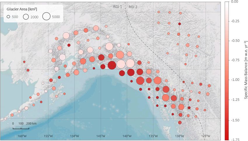
1848                       L. Jakob et al.: Ice loss in High Mountain Asia and the Gulf of Alaska between 2010 and 2019

2     Data and methods                                             2.2   Rates of elevation change maps

In this section, we give a short overview of the data and meth-    Rates of elevation change and mass balance are based on
ods used in this study. More details can be found in the Sup-      ∼ 25 million swath elevation measurements in the GoA re-
plement.                                                           gion and ∼ 8 million swath elevation measurements in HMA
                                                                   acquired from July 2010 to July 2019. The distribution of el-
2.1    Time-dependent elevation from CryoSat-2                     evation measurements with altitude departs somewhat from
       observations                                                the glaciers’ hypsometry. Hypsometric representativeness of
                                                                   samples within spatial units is a key requirement for robust
We use observations from the SAR (synthetic aperture radar)
                                                                   glacier trend estimates. A bias in the altitudinal distribution
Interferometric Radar Altimeter (SIRAL) on board the Euro-
                                                                   of observations can lead to a bias in the total rate of thinning
pean Space Agency (ESA) CryoSat-2 satellite (Wingham et
                                                                   when integrated over a larger domain as rate of thickness
al., 2006). SIRAL is a beam-forming active microwave radar
                                                                   change is often strongly correlated with altitude. Therefore
altimeter with a maximum imaging range of ∼ 15 km on the
                                                                   we derive a subset of the time-dependent elevation dataset,
ground. The sensor emits time-limited Ku-band pulses aimed
                                                                   removing the impact of such point density biases by filter-
at reducing the footprint to ∼ 1.6 km within the beam. Over
                                                                   ing out swath measurements so as to match the glacier hyp-
land ice, the sensor operates in synthetic aperture interfero-
                                                                   sometry binned using 100 m elevation intervals (e.g. Treich-
metric (SARIn) mode, which allows delay-Doppler process-
                                                                   ler et al., 2019), and generate elevation change and mass
ing to generate an along-track footprint of ∼ 380 m, while
                                                                   change estimates from the reduced sample (Fig. S5). We re-
cross-track interferometry is used to extract key information
                                                                   move data sequentially based on measurement uncertainty.
about the position of the footprint centre. In practice how-
                                                                   This process reduces our sample size by 15 % for the GoA
ever, footprint size will vary depending on properties such
                                                                   and by 30 % for HMA. We then follow a similar approach
as surface slopes, scattering properties, and distance from
                                                                   to Foresta et al. (2016) and Gourmelen et al. (2018); how-
the point of closest approach (POCA). CryoSat-2 orbits the
                                                                   ever the lower data density and the complexity of the ter-
Earth with a 369 d near-repeat period formed by the succes-
                                                                   rain in the GoA region and in HMA require a slight adapta-
sive shift in a 30 d sub-cycle. The satellite has an inclination
                                                                   tion of the methodology. We bin the elevation measurements
of 92◦ , offering improved coverage of the polar regions. We
                                                                   into regions of 100 × 100 km, sufficiently large to contain
process level 1b, baseline C data and the corrected mispoint-
                                                                   the necessary number of measurements in each bin to en-
ing angle for aberration of light (Scagliola et al., 2018) sup-
                                                                   sure sufficient robustness and representativity. Due to the in-
plied by the ESA ground segment using a swath processing
                                                                   creased bin size (the pixel size used by Foresta et al., 2016,
algorithm (Gourmelen et al., 2018). Level 1b data are pro-
                                                                   and Gourmelen et al., 2018, is 1000 m) and the variation in
vided as a sequence of radar echoes along the satellite track,
                                                                   elevations within each bin, the topographic signature can-
which translates into received power, interferometric phase,
                                                                   not simply be modelled and therefore needs to be removed
and coherence waveforms for each along-track location. The
                                                                   using an auxiliary digital elevation model (DEM) (Kääb et
conventional level 1b data processing method consists of ex-
                                                                   al., 2012). We subtract the TanDEM-X 90 m DEM (German
tracting single elevation measurements from the power sig-
                                                                   Aerospace Center (DLR), 2018), which has a near-complete
nal in each waveform that corresponds to the POCA between
                                                                   coverage and is contemporaneous with the CryoSat-2 obser-
the satellite and the ground. In contrast, swath altimetry ex-
                                                                   vations, from the swath elevation measurements. The remain-
ploits the full radar waveform to map a dense swath (∼ 5 km
                                                                   ing elevation differences (hereinafter referred to as elevDiff)
wide) of elevation measurements across the satellite ground
                                                                   are due to time-dependent elevation change that can be re-
track beyond POCA (Foresta et al., 2016, 2018; Gourmelen
                                                                   lated to glacier thickness change as well as errors in the two
et al., 2018; Gray et al., 2013; Hawley et al., 2009), provid-
                                                                   datasets, temporal heterogeneity (TanDEM-X is a composite
ing 1 to 2 orders of magnitude more elevation measurements
                                                                   of acquisitions from different years), and differences in pen-
compared with POCA and improving the sampling of topo-
                                                                   etration between the reference DEM (X-band) and the swath
graphic lows (Foresta et al., 2016). Because swath processing
                                                                   elevation measurements. The errors related to the reference
does not rely on retracking, it can retrieve elevation measure-
                                                                   DEM will result in an increase in spread of the elevDiff mea-
ments also for atypical waveforms with no clearly defined
                                                                   surements and are accounted for in the regression model dis-
leading edge such as those found over complex terrain and
                                                                   cussed below.
where retracking often fails to identify a reliable POCA. This
                                                                      Rates of elevation change are then calculated for each
makes the CryoSat-2 sensor at present the only radar altime-
                                                                   100 × 100 km bin individually based on elevDiff measure-
ter able to survey glaciers at high resolution.
                                                                   ments from July 2010 to July 2019. In order to achieve the
                                                                   most robust trends, we considered several fitting methods, in-
                                                                   cluding ordinary least squares, robust regression (e.g. Kääb
                                                                   et al., 2012, 2015), weighted regression (e.g. Berthier et al.,
                                                                   2016; Foresta et al., 2018; Gourmelen et al., 2018), random

The Cryosphere, 15, 1845–1862, 2021                                                   https://doi.org/10.5194/tc-15-1845-2021
L. Jakob et al.: Ice loss in High Mountain Asia and the Gulf of Alaska between 2010 and 2019                                 1849

sample consensus (RANSAC), and the Theil–Sen estimator            ries of the 100 × 100 km bins are also used as an additional
(e.g. Shean et al., 2020). We found that the best results were    check of the dh/dt quality (see Sect. S1.2), whilst we exploit
achieved with a weighted regression model of the elevD-           the sub-regional and regional time series to analyse spatio-
iff measurements, similar to the methods of Gourmelen et          temporal variability in thickness change across both the GoA
al. (2018). However, whilst their weights are calculated only     and HMA regions. To generate region-wide time series for
according to the power attribute, here we assign each obser-      HMA and the GoA, we use an area-weighted mean of the
vation a weight based on power and coherence; i.e. measure-       sub-regional time series. Note that, as opposed to the linear
ments with high power and low coherence within the sam-           rates, the regional and sub-regional time series displayed in
ple will have lower weights assigned (see Sect. S1.1 in the       this publication start in January 2011 (with the earliest data
Supplement). We exclude solutions that display extremely          from November 2010 using the 90 d window) since we re-
large variability across various regression models, consider-     trieve fewer swath measurements for the first few months of
ing them to be unstable results (see Sect. S1.2). When fit-       CryoSat-2’s life cycle, impacting the quality of the time se-
ting the model, we iteratively exclude measurements that are      ries pre-2011. The time series in this paper end in April 2019,
more than 3σ from the mean distance to the fitted line until      with the latest data from June 2019 due to the 90 d window.
no more outliers are present (e.g. Foresta et al., 2016, 2018).
We discard bins that did not fulfil a set of quality criteria     2.5   Uncertainty assessment
based on elevation change uncertainties, temporal complete-
ness, interannual changes, and stability of regression results    The error budget of mass change has three uncertainty
(see Sect. S1.2). The remaining bins covered more than 96 %       sources, which are assumed to be independent and uncorre-
of the total glacierized area in the GoA region and 88 % in       lated: uncertainty in time-dependent elevation change (σ1h ),
HMA. To estimate values for the gaps in our dh/dt map,            uncertainty in glacierized area A (σA ), and uncertainty in
we use the altitudinal distribution of elevation change rates     mass–volume conversion (σp ).
on a sub-regional level (Moholdt et al., 2010a, b; Nilsson et        The rate of elevation change uncertainty for each
al., 2015), applying the hypsometric averaging methods de-        100 × 100 km bin is based on the standard error of the re-
scribed in Sect. S1.3.                                            gression model. We conservatively use a factor of 5 (Berthier
                                                                  et al., 2014; Brun et al., 2017) for uncertainties in areas with-
2.3   Mass balance and contribution to sea level rise             out coverage of swath measurements:

To obtain volume changes we use the glacierized area              σ1h = σ1z (g + 5u),                                          (1)
of the Randolph Glacier Inventory (RGI 6.0) (RGI Con-
sortium, 2017). We assume a standard bulk density of              where g is the proportional coverage of glacierized area at
850 ± 60 kg m−3 (Huss, 2013) to convert volume changes            400 m postings, u is (1 − g), and σ1z is the standard error
to equivalent mass changes. This assumption is consid-            of the regression. To retrieve the uncertainty in extrapolated
ered appropriate for a wide range of conditions and longer-       bins, we calculate the differences in all non-extrapolated bins
term trends; however, this factor can differ significantly for    between elevation changes using the plane fit approach and
shorter-term periods (< 3 years) (Huss, 2013). To obtain a        elevation changes using the hypsometric averaging method.
region-wide mass balance, mass changes in each individ-           The standard deviation of these differences is the uncertainty
ual bin are summed up. To generate the contribution to            in elevation change (σ1h ) for all extrapolated bins. We re-
sea level rise (SLR), we assume an area of the ocean of           trieve an uncertainty in elevation change for extrapolated
361.8 × 10⁶ km2 and consider total contributions from all         bins of 0.34 and 0.47 m yr−1 , respectively, for High Moun-
glaciers and then only those glaciers within exorheic basins      tain Asia and the Gulf of Alaska. To account for errors due to
in High Mountain Asia, based on the HydroSHEDS dataset            temporal changes in glacier extents and polygon digitization
(Lehner et al., 2006).                                            (Shean et al., 2020), we use an error of 10 % (σA = 0.1A) in
                                                                  the glacierized area A in a bin, even though the reported un-
2.4   Time series of surface elevation changes                    certainty in the RGI is ∼ 8 % (Pfeffer et al., 2014). Assuming
                                                                  independence between the two error components (σA , σ1h ),
CryoSat-2’s monthly repeat cycle provides the opportunity         volume change uncertainty (σ1V ) of a bin is
to monitor seasonal as well as multiannual trends of surface              p                       2
elevation. We therefore generate time series with a monthly       σ1V =       (σ1h A)2 + (σA 1h) ,                             (2)
step (30 d) and a 3-month (90 d) moving window using the
median of all the elevDiff observations (residuals from the       where 1h is the elevation change rate of the respective bin.
reference DEM) within a time period with reference to the         To generate the region-wide volume uncertainty (σ1Vtot ),
first month. Time series are generated at the bin size level      we combine all the values (including extrapolated bins) in
(100 × 100 km), at the sub-regional level (using the RGI          quadrature. We use a density uncertainty of σp = 60 kg m−3
sub-regions), and for the full study region. The time se-         and a density mass conversion of p = 850 kg m−3 (Huss,

https://doi.org/10.5194/tc-15-1845-2021                                                 The Cryosphere, 15, 1845–1862, 2021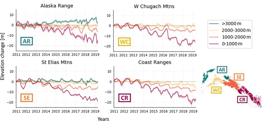
1850                           L. Jakob et al.: Ice loss in High Mountain Asia and the Gulf of Alaska between 2010 and 2019

2013). The total mass balance uncertainty is                       feature is the gradient from moderate thinning in Spiti–
                                                                   Lahaul and western Himalaya (−0.25 ± 0.09 m w.e. yr−1 ) to
                                         2
                                                                   increasingly negative surface elevation changes along
           q
σ1Mtot =        (σ1Vtot p)2 + (σp 1Vtot ) ,                (3)
                                                                   the central (−0.43 ± 0.14 m w.e. yr−1 ) and eastern
                                                                   (−0.56 ± 0.16 m w.e. yr−1 ) Himalayan mountain range,
where 1Vtot is the total volume change for the region.
                                                                   with the Nyainqêntanglha Mountains and Hengduan Shan
                                                                   (−0.98 ± 0.22 m w.e. yr−1 ) showing the highest negative
3     Results                                                      trends (Table 1).
                                                                      We display the altitudinal distribution of elevation changes
3.1    Spatial coverage and elevation sampling                     in Fig. 6 and a comparison with Brun et al. (2017) in Fig. S7.
                                                                   While some variability exists along the profiles, in particular
Using the theoretical pulse-limited footprint size of CryoSat-     over regions and elevation ranges containing fewer glaciers
2, we derive a total spatial coverage of glaciated regions of      that can reflect a less robust solution and/or spatial variability
55 % in the GoA and 32 % in HMA, respectively. These val-          in glacier response, trends between elevation and ice thick-
ues are the combined result of the absence of recorded re-         ness change are clearly visible. In general, we observe de-
turns due to orbit separation and onboard-tracking limitation      creasing negative trends with increasing altitudes, which is
(Dehecq et al., 2013) as well as data quality. Given that it is    an expected pattern (Brun et al., 2017; Gardelle et al., 2013).
estimated that 40 % of HMA glaciers are not sampled due to         We find the steepest gradient (Fig. 6, S7, Table S4) in the
onboard-tracking limitations (Dehecq et al., 2013) we esti-        Nyainqêntanglha or Hengduan Shan, which is in line with
mate that with an appropriate onboard-tracking system, the         the findings of Brun et al. (2017). We also observe lower or
rate coverage for HMA would be as high as 50 %. These              even inverse gradients in Bhutan or eastern Himalaya, Spiti–
values are within the high end of the range of observational       Lahaul or western Himalaya, Karakoram or western Kunlun,
methods (Zemp et al., 2019) whilst generally lower than the        and Pamir (Figs. 6, S7, Table S4), which have been reported
coverage provided by high-resolution sensors (Brun et al.,         previously and been related to debris thickness (Bisset et al.,
2017; Shean et al., 2020). As expected from the relatively         2020; Brun et al., 2017).
large footprint of radar altimeters, we observe a positive cor-       We show temporal variability in surface elevation change
relation between spatial coverage and glacier size; we do          for the whole HMA region (Fig. 4), the RGI second-order
however observe coverage over all glacier sizes (Fig. S6).         regions (Figs. 5, S1), and the regions by Brun et al. (2017)
   We observe a bias in the total number of swath mea-             (Fig. S2). The monthly time series show sustained multian-
surements towards higher altitudes (e.g. Fig. S5), which can       nual trends across almost all of the sub-regions until 2015–
be attributed to the onboard tracking tending to favour el-        2016 and decreased loss or even mass gain from 2016–2017
evations closest to the satellite. However, a comparison of        onwards (Figs. 5, S2), which is also reflected in the full HMA
the glacier hypsometry and the spatial coverage of our data        time series (Fig. 4) and consistent with previous observations
(Fig. S4) shows that we still achieve good coverage at low el-     (Ciracì et al., 2020). The Karakoram region in particular dis-
evations in both regions. In addition, we interpolate missing      plays thinning from 2011 to 2014–2015 before abating and
data based on the relationship between elevation and eleva-        thickening again from 2016–2017. This shift in thinning rates
tion changes and therefore still capture the changes in the        post-2015 is also clearly seen in Bhutan or eastern Himalaya,
lower reaches of the HMA and GoA glaciers.                         Kunlun (west and east), Tien Shan, Pamir Alay or Hissar
                                                                   Alay, and Nyainqêntanglha or Hengduan Shan (Figs. 5, S1,
3.2    Elevation changes and mass balance in High                  S2).
       Mountain Asia
                                                                   3.3   Glacier elevation changes and mass balance in the
The total HMA mass balance between 2010 and 2019                         Gulf of Alaska
was −28.0 ± 3.0 Gt yr−1 (−0.29 ± 0.03 m w.e. yr−1 ), or
−18.3 ± 2.3 Gt yr−1 (−0.38 ± 0.03 m w.e. yr−1 ) when in-           In general, we find much higher mass losses in the Gulf
cluding only exorheic basins. This mass loss corresponds           of Alaska than in High Mountain Asia. Over an area of
to 0.078 ± 0.008 mm yr−1 SLE, or 0.051 ± 0.006 mm yr−1             ∼ 86 000 km2 , including all 26 490 glaciers in the RGI
when including only exorheic basins, and a cumulative              region 1 except northern Alaska, we estimate a total mass
loss of 4.2 % of the total ice volume in High Mountain             balance of −76.3 ± 5.7 Gt yr−1 (−0.89 ± 0.07 m w.e. yr−1 ),
Asia during the study period (Farinotti et al., 2019). Our         contributing −0.211 ± 0.016 mm yr−1 to global sea level
maps of surface elevation change show a heterogeneous              rise, corresponding to a cumulative loss of 4.3 % of the
pattern in the Himalayan range, with a cluster of slightly         total ice volume during the study period (Farinotti et al.,
positive and near-balance trends in the Kunlun and Karako-         2019). Surface elevation change maps (Fig. 3) display
ram ranges (Fig. 2), the so-called “Karakoram anomaly”             an expected pattern, with more negative trends towards
(Gardelle et al., 2012; Hewitt, 2005). Another striking            lower elevations close to the coast. Note that some of

The Cryosphere, 15, 1845–1862, 2021                                                    https://doi.org/10.5194/tc-15-1845-2021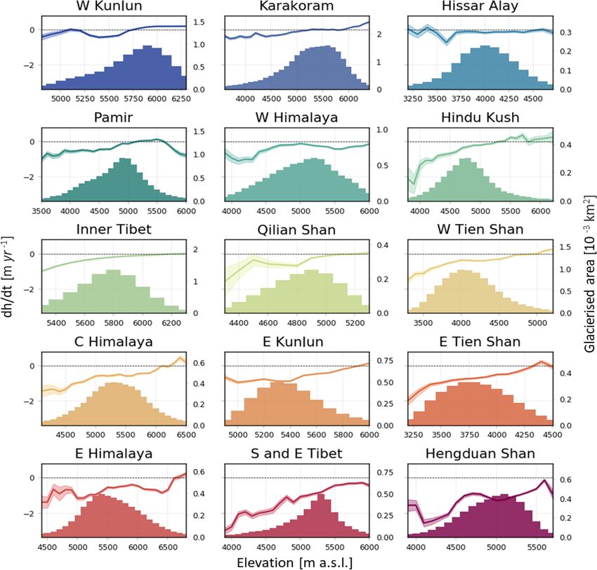
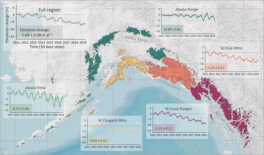
L. Jakob et al.: Ice loss in High Mountain Asia and the Gulf of Alaska between 2010 and 2019                                                  1851

Figure 2. Specific glacier mass balance (m w.e. yr−1 ) in High Mountain Asia (HMA) for the period of July 2010 to July 2019 on a
100 × 100 km grid. The size of the circles is scaled by the total glacierized area within a 100 × 100 km bin.

Figure 3. Specific glacier mass balance (m w.e. yr−1 ) in the Gulf of Alaska (GoA) for the period of July 2010 to July 2019 on a 100 × 100 km
grid. The size of the circles is scaled by the total glacierized area within a cell. Note that our total mass change estimate of −76.3 ± 5.7 Gt yr−1
(−0.89 ± 0.07 m w.e. yr−1 ) only includes glaciers from the RGI region 1 (Alaska). Including also the northern Rocky Mountains and the
Mackenzie and Selwyn mountains, we retrieve a mass change of −77.7 ± 5.7 Gt yr−1 .

the lower rates observed in the Saint Elias Mountains are                   ble 2. The largest mass loss is seen in the northern Coast
likely the result of the presence of accumulation areas of                  Ranges (−1.08 ± 0.09 m w.e. yr−1 , −24.8 ± 2.1 Gt yr−1 )
large glaciers, e.g. Hubbard and Bering glaciers in these                   and Saint Elias Mountains (−1.03 ± 0.10 m w.e. yr−1 ,
particular grid cells. We present sub-regional estimates                    −34.1 ± 3.4 Gt yr−1 ), especially in the Yukutat and Glacier
aggregated in the RGI 6.0 second-order regions in Ta-                       Bay region, which is in line with the spatial patterns of

https://doi.org/10.5194/tc-15-1845-2021                                                              The Cryosphere, 15, 1845–1862, 2021
1852                        L. Jakob et al.: Ice loss in High Mountain Asia and the Gulf of Alaska between 2010 and 2019

Table 2. Gulf of Alaska (GoA) mass balance trends from July 2010 to July 2019, aggregated on the Randolph Glacier Inventory (RGI 6.0)
sub-regions.

                                                                Glacier area    Specific mass change     Mass change
                                                                      (km2 )            (m w.e. yr−1 )     (Gt yr−1 )
                    Alaska Range (Wrangell and Kilbuck)              16278              −0.41 ± 0.05      −6.6 ± 0.9
                    Alaska Pena (Aleutians)                           1912              −0.64 ± 0.10      −1.2 ± 0.2
                    Western Chugach Mountains (Talkeetna)            12 052             −0.80 ± 0.09      −9.6 ± 1.0
                    Saint Elias Mountains                            33 174             −1.03 ± 0.10     −34.1 ± 3.4
                    Northern Coast Ranges                            22 963             −1.08 ± 0.09     −24.8 ± 2.1
                    Total                                            86 379

Figure 4. Monthly surface elevation change time series for High Mountain Asia (a) and the Gulf of Alaska (GoA) region (b). The grey lines
display the elevation change time series with the uncertainty envelope. The red line displays a 12-month moving average.

Luthcke et al. (2008) and Luthcke et al. (2013). The lowest            4     Discussion
thinning rates are observed in the Alaska Range mountains
(−0.41 ± 0.05 m w.e. yr−1 ), which is also in agreement with           4.1     Uncertainty
other studies (Berthier et al., 2010; Luthcke et al., 2008).
We observe a clear correlation between surface elevation               While our uncertainty methods follow existing approaches,
changes and altitude (Fig. 11, Table S2), with the highest             and our error bounds are similar in magnitude to Brun et
negative trends at low altitudes in the Saint Elias Mountains          al. (2017), Kääb et al. (2012), and Shean et al. (2020) but
and Coast Ranges.                                                      lower than GRACE-based estimates, several additional po-
   We display temporal variability in surface elevation                tential sources of errors could impact the results. Radar al-
change for the whole GoA region (Fig. 4), the RGI sub-                 timetry – delay-Doppler radar in particular – has been shown
regions (Figs. 9, S3), and for different elevation bands within        to be sensitive to surface slopes, in particular to slopes in the
sub-regions (Fig. 10). Figure 9 shows negative trends across           direction of the satellite’s flight path. In regions like HMA
all the sub-regions. The four coastal sub-regions – Alaska             and GoA, this impact will also be seen in the performance
Pena, western Chugach Mountains, Saint Elias Mountains,                of the onboard tracker as, for large slopes, the system is ex-
and Coast Ranges – display a seasonal oscillation, with an             pected to “lose lock”. While we observe a decreased cover-
annual surface elevation maximum in spring and annual sur-             age compared to other, less mountainous, glaciated regions,
face elevation minimum in autumn. In contrast, the seasonal            we also demonstrate here that measurements do cover the en-
cycle of the Alaska Range mountains is shifted, with the               tire elevation range of glaciers in the HMA and GoA regions,
thickness maximum in winter, which is also somewhat vis-               allowing us to match the glaciers’ hypsometry. We also do
ible in the time series by Luthcke et al. (2008). A very no-           not observe significant coverage bias as a function of glacier
ticeable feature within the full GoA time series is the accel-         orientation with respect to the satellite’s track path. The spa-
eration of thinning from 2013 to 2014 onwards (Fig. 4). We             tial coverage is such that we demonstrably resolve spatial,
record an acceleration of thinning from −0.06 ± 0.33 m yr−1            altitudinal, and temporal evolution of glacier elevation.
(January 2011 to January 2013) to −1.1 ± 0.06 m yr−1 (Jan-                It is a well-known observation that microwave pulses scat-
uary 2013 to January 2019). We observe this almost consis-             ter from the surface as well as the subsurface, which can lead
tently across the five sub-regions, but this is most pronounced        to elevation change bias in regions of historically anomalous
in the Saint Elias Mountains, the western Chugach Moun-                melt events (Nilsson et al., 2015) or at a seasonal timescale
tains, and the Coast Ranges.                                           (Gray et al., 2019). Over most regions however, it has been
                                                                       shown that surface elevation change from CryoSat over an-

The Cryosphere, 15, 1845–1862, 2021                                                          https://doi.org/10.5194/tc-15-1845-2021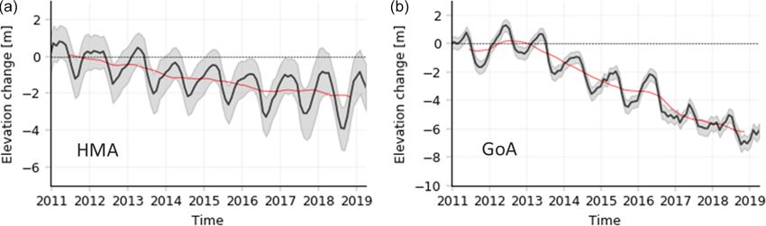
L. Jakob et al.: Ice loss in High Mountain Asia and the Gulf of Alaska between 2010 and 2019                                            1853

Figure 5. High Mountain Asia (HMA) 30 d elevation change time series in the RGI 6.0 second-order regions. The coloured line displays the
time series with the uncertainty envelope (y axis: elevation change [m]; x axis: time [30 d steps]). The numbers describe the elevation change
with uncertainties in m yr−1 .

nual and pluri-annual timescale is consistent with in situ, air-         4.2     High Mountain Asia
borne, and meteorological observations (Gourmelen et al.,
2018; Gray et al., 2015, 2019; McMillan et al., 2014a; Zheng             4.2.1    Temporal variability
et al., 2018). Using static glacier masks can also lead to er-
rors in regions of rapid dynamic changes. In general, these
                                                                         The seasonal and annual time series variability reflects the in-
limitations are known, and efforts are currently underway in
                                                                         fluence of atmospheric circulations and precipitation season-
the community to improve uncertainty analysis and develop
                                                                         ality in High Mountain Asia on ice thickness change. Sub-
new glacier outline products (RAGMAC, 2019).
                                                                         regions dominated by winter accumulation (generally west-
   Although the time series generally reflect the actual
                                                                         erly regimes), such as the Hindu Kush, western Himalaya,
change in surface elevation, there are a number of limita-
                                                                         and the Pamir region (Pohl et al., 2015; Yao et al., 2012),
tions that are important to keep in mind when interpreting
                                                                         show the typical seasonal pattern with mass accumulation
the results from radar altimetry. For the reasons stated above,
                                                                         during winter and early spring and mass losses in the summer
scattering properties can induce elevation biases at a sea-
                                                                         and autumn months (Fig. 5).
sonal timescale (Gray et al., 2019). In addition, integrating
                                                                            Contrarily, sub-regions such as central Himalaya, eastern
changes over large regions can lead to spatial heterogeneity
                                                                         Himalaya, and Hengduan Shan show a more heterogeneous
in the successive time steps, in particular when the data vol-
                                                                         seasonal pattern. The elevation change time series of these
ume becomes too low. These limitations may explain some
                                                                         three sub-regions indicate that the annual cycle has two max-
of the observed patterns and in particular the few cases where
                                                                         ima, with a first maximum in winter and a second and smaller
seasonal variability is larger than what is expected from our
                                                                         peak in summer (Figs. 5, S1). Receiving summer accumula-
knowledge of SMB (surface mass balance) in the regions.
                                                                         tion through the Indian monsoon, these sub-regions generally
                                                                         have a precipitation maximum in July or August; however
                                                                         they are also defined by a high variability in precipitation
                                                                         regimes (Maussion et al., 2014) and a high temperature range
                                                                         (Sakai and Fujita, 2017), resulting in glaciers with varying

https://doi.org/10.5194/tc-15-1845-2021                                                          The Cryosphere, 15, 1845–1862, 2021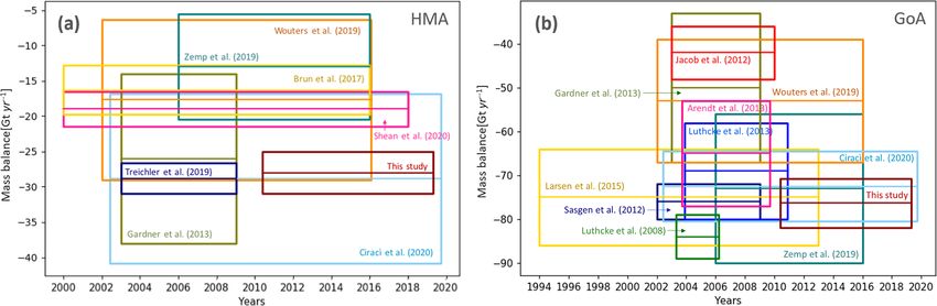
1854                         L. Jakob et al.: Ice loss in High Mountain Asia and the Gulf of Alaska between 2010 and 2019

                                                                       the −28.8 ± 12 Gt yr−1 by Ciracì et al. (2020), a study based
                                                                       on the GRACE and GRACE Follow-On mission covering
                                                                       the period of 2002 to 2019. The results are similar to the
                                                                       estimates provided by various ICESat studies for the years
                                                                       2003 to 2008, including the −28.8±2.2 Gt yr−1 by Treichler
                                                                       et al. (2019), the −24 ± 2 Gt yr−1 by Kääb et al. (2015)
                                                                       (excludes the Tien Shan and the inner Tibetan Plateau), and
                                                                       the −26 ± 12 Gt yr−1 by Gardner et al. (2013) (based on
                                                                       ICESat and GRACE). Our estimates are higher than recent
                                                                       DEM differencing studies such as the −19.0 ± 2.5 Gt yr−1
                                                                       (−0.19 ± 0.03 m w.e. yr−1 ) by Shean et al. (2020) and the
                                                                       −16.3 ± 3.5 Gt yr−1 (−0.16 ± 0.08 m w.e. yr−1 ) by Brun et
                                                                       al. (2017).
                                                                          Besides the differences in data and methodology, a part
                                                                       of these disagreements can be explained by the time peri-
                                                                       ods. Maurer et al. (2019) and King et al. (2019) find that the
                                                                       thinning rates in the Himalayas have increased from the in-
                                                                       terval 1975–2000 to 2000–2016. This trend seems to have
                                                                       continued in more recent years, with Ciracì et al. (2020)
                                                                       observing significant variation in rates of mass loss during
Figure 6. Altitudinal distribution of elevation changes and glacier    the period between 2002 and 2019, with mean rates of loss
hypsometry functions in High Mountain Asia (HMA) in RGI 6.0            35 % larger during the CryoSat period than between 2002
sub-regions between 2010 and 2019. The lines show elevation
                                                                       and 2010, which could explain our more negative mass bal-
change rates with uncertainty envelopes plotted against 100 m el-
                                                                       ance in comparison to Brun et al. (2017) (2000 to 2016) and
evation bands (left y axis). The bars display the glacier hypsometry
(right y axis).                                                        Shean et al. (2020) (2000 to 2018).

                                                                       4.2.3   Comparison of sub-regional mass balances with
types over very short distances (Maussion et al., 2014). The                   previous work
impact of this variability becomes evident when compared
to the more periodic seasonal patterns of the Hindu Kush,              Our higher regional mass loss when comparing to the two
western Himalayas, and Pamir time series. This also stands             DEM differencing studies by Brun et al. (2017) and Shean
in contrast with the inner Tibetan Plateau, dominated by a             et al. (2020) is mostly due to differences in the south-eastern
more continental climate, where glaciers exhibit almost no             Himalaya – especially Nyainqêntanglha or Hengduan Shan
intra-annual cycle.                                                    – and in the Pamir regions. We used the regions by Brun et
   In general, the heterogeneity of the time series reflects the       al. (2017), the RGI 6.0 second-order regions, and the HiMAP
sensitivity of mountain glaciers to meteorological patterns            (Hindu Kush Himalayan Monitoring and Assessment Pro-
and changes and emphasizes that glaciers in High Mountain              gramme) regions (Bolch et al., 2019) to compare our results
Asia cannot be considered to be one entity with uniform tem-           with other estimates (Figs. 7, S8, S9 and Tables S1, S2). For
poral variability and sensitivity to changes.                          a full discussion of regional differences between estimates of
                                                                       recent studies, refer to Bolch et al. (2019). Our results are in
4.2.2   Comparison of regional mass balance with                       line with general findings by Bolch et al. (2019) in the sense
        previous work                                                  that we obtain similar results in sub-regions where there is
                                                                       a good agreement in general between studies, such as Tien
A comparison of mass balance results in the literature indi-           Shan, Karakoram, western Nepal (western Himalaya), and
cates that, while all the studies agree on the general trend           Hindu Kush. For Nyainqêntanglha (named Hengduan Shan
in mass loss and spatial variability in mass loss, there is a          and southern and eastern Tibet in the RGI sub-region masks)
large degree of variability between estimates. While some of           – one of the most controversial regions – Shean et al. (2020)
the variability can be attributed to the diversity of time spans       and Brun et al. (2017) report significantly less negative mass
and regional boundaries used, there are also clear differences         trends (−0.50 ± 0.15 and −0.62 ± 0.23 m w.e. yr−1 ) than our
between observation methods (Fig. 8a). Note that here we               estimates of −0.97 ± 0.19 m w.e. yr−1 , whilst in situ mea-
are only comparing region-wide mass trends with the results            surements (−0.94 m w.e. yr−1 by Yao et al., 2012, based on
closest in space and time to this study, whilst sub-regional           the Parlung glaciers between 2006 and 2010) and ICESat
differences are discussed in the next section.                         studies (Kääb et al., 2015; Treichler et al., 2019) find higher
   Our total mass balance of −28.0 ± 3.0 Gt yr−1                       negative rates for the survey time period of 2003 to 2008. We
(−0.29 ± 0.03 m w.e. yr−1 ) is in good agreement with                  also record higher mass losses in eastern Himalaya/Bhutan,

The Cryosphere, 15, 1845–1862, 2021                                                       https://doi.org/10.5194/tc-15-1845-2021
L. Jakob et al.: Ice loss in High Mountain Asia and the Gulf of Alaska between 2010 and 2019 1855 Figure 7. High Mountain Asia (HMA) specific mass balance trends on a sub-regional level (using the sub-regions of Brun et al., 2017) in comparison with DEM differencing and ICESat studies. It is important to note that Shean et al. (2020) cover the time period of 2000 to 2018, Brun et al. (2017) cover the time period of 2000 to 2016, and Kääb et al. (2015) cover the time period 2003 to 2008, whilst this study covers the time period of July 2010 to July 2019. We have complemented the data from Kääb et al. (2015) with ICESat data from Brun et al. (2017) for the sub-regions Kunlun, inner TP (Tibetan Plateau), Tien Shan and Pamir Alay, which extended the estimates of Kääb et al. (2015) using the same method. adjacent to the Nyainqêntanglha Mountains. The differences creased mass loss from January 2015 onwards, which could in Nyainqêntanglha and eastern Himalaya between our es- account for the higher mass loss estimates in comparison to timates and the ones of Brun et al. (2017) and Shean et the DEM differencing studies covering the last 2 decades al. (2020) (time periods 2000–2016 and 2000–2018) fit in (Brun et al., 2017; Gardelle et al., 2013; Shean et al., 2020). with the generally observed acceleration of mass loss in The spatial thinning pattern in the Kunlun–Karakoram South East Asia over the past decades (Maurer et al., 2019; area (Fig. 2) confirms the suggestion of previous studies Zemp et al., 2019). Some studies suggest the weakening of (Brun et al., 2017; Gardner et al., 2013; Kääb et al., 2015) the Indian summer monsoon as the primary source of in- that the so-called “Karakoram anomaly” (Gardelle et al., creased thinning (Salerno et al., 2015), whilst other stud- 2012; Hewitt, 2005) stretches up to western Kunlun Shan, ies find no widespread precipitation decrease in monsoonal which is now considered the centre of the anomaly. We regimes, which could account for all of these changes and record less mass gain in Kunlun (+0.01 ± 0.05 m w.e. yr−1 , attribute the temperature sensitivity of glaciers in monsoon- +0.06 ± 0.05 m w.e. yr−1 in the western part of Kunlun) than dominated regions as the main driver (Maurer et al., 2019). In previous studies, indicating that the Karakoram anomaly fact, glaciers in Hengduan Shan, Nyainqêntanglha, and east- might not persist long-term (Farinotti et al., 2020; Rounce ern Himalaya have been found to exhibit the highest sensi- et al., 2020). This observation is also reflected in the ele- tivity towards temperature in the whole HMA region (Sakai vation change profile of the Kunlun regions, where Brun et and Fujita, 2017). al. (2017) find constant thickening at almost all elevations Contrasting estimates have also been published for the during the survey time period of 2000 to 2016, whilst we Pamir and Pamir Alay mountains (Hissar Alay), where high record thinning at lower elevations (see Fig. S7). These find- (Kääb et al., 2015), moderate (this study; Ciracì et al., 2020; ings suggest a shift towards negative mass balance at lower Gardner et al., 2013), and slight mass losses (Brun et al., elevations in the Kunlun region in comparison to the pre- 2017; Shean et al., 2020) and even mass gains (Gardelle et vious decade. However, our time series suggests increased al., 2013) have been reported. Part of the discrepancy can be mass gain from 2016 in western Kunlun and also mass gain attributed to time variability in mass loss (Brun et al., 2017) in the Karakoram (Fig. 5). At the same time, we also ob- and driven by fluctuation in winter precipitation (Smith and serve decreased thinning rates in inner Tibet and eastern Bookhagen, 2018). CryoSat time series indeed suggest in- Kunlun. These changes could be a short-term trend; however, https://doi.org/10.5194/tc-15-1845-2021 The Cryosphere, 15, 1845–1862, 2021
1856 L. Jakob et al.: Ice loss in High Mountain Asia and the Gulf of Alaska between 2010 and 2019
Figure 8. Estimates of mass balance [Gt yr−1 ] as published in different studies for High Mountain Asia (a) and Alaska (b).
it displays the limitation of all mentioned studies (including −69 ± 11 Gt yr−1 by Sasgen et al., 2012, Ciracì et al., 2020,
this study) when deriving linear trends in a region like High and Luthcke et al., 2013) and ICESat (−65 ± 12 Gt yr−1 by
Mountain Asia with large interannual climate variability and Arendt et al., 2013) as well as a study from airborne altimetry
associated glacier changes. (−75 ± 11 Gt yr−1 by Larsen et al., 2015) and a consensus
We generally find better agreements with Shean et estimate combining glaciological and geodetic observa-
al. (2020), the study including an additional 2+ years (2017 tions (−73 ± 17 Gt yr−1 , or −0.85 ± 0.19 m w.e. yr−1 by
and 2018) in comparison to Brun et al. (2017) and thus more Zemp et al., 2019) (Fig. 8b). Our result is significantly
closely aligned with our time period. This potentially indi- more negative than two GRACE studies, with estimates of
cates that a large part of the disagreements could be related −53 ± 14 Gt yr−1 (Wouters et al., 2019) and −42±6 Gt yr−1
to interannual variability and survey time period. (Jacob et al., 2012). Besides the variations in methodologies
and data between these studies, also differences in study
4.3 Gulf of Alaska area extents, glacier masks, and volume-to-mass conversion
factors contribute to the spread of total mass change results.
4.3.1 Temporal variability Our estimates correspond to the RGI region 1 (excluding
northern Alaska) to make the results more comparable for
The increased thinning from 2013–2014 onwards (see future studies. In general, our total mass balance is more
Figs. 4, 9, S3), which we observed across all sub-regions, negative than most other studies’ findings, reflecting the
has also been reported by Wouters et al. (2019) and Ciracì et increased thinning rates we show in the sub-regional time
al. (2020) in GRACE time series covering the whole Alaska series from 2013–2014.
region. This change correlates with the change from a nega-
tive PDO phase to a positive phase in 2013–2014, which re- 4.3.3 Comparison of sub-regional mass balances with
sulted in increased temperatures (Wendler et al., 2017). This previous work
is in agreement with Wouters et al. (2019), finding that their
interannual mass change variations negatively correlate with Since there is no prevalent sub-region mask used by more
the May–September PDO and May–August NAO (North recent studies, we cannot directly compare and validate our
Atlantic Oscillation) indices. Our findings further suggest results on a sub-regional level. Mass balance or surface el-
that the sensitivity of glaciers to the 2013–2014 temperature evation change estimates that overlap with our time period
change increases towards lower elevations (Fig. 10). The fact are either spatially not resolved (e.g. Gardner et al., 2013;
that the strongest impact is observed in the coastal regions Zemp et al., 2019), presented on a glacier-to-glacier basis
is likely due to the higher sensitivity of maritime glaciers (e.g. Larsen et al., 2015), or GRACE mascon extents (e.g.
in Alaska to temperature change (Gregory and Oerlemans, Luthcke et al., 2008, 2013).
1998) and the lower elevations within these regions. Figure 12 displays a comparison with the 1962–2006 es-
timates of Berthier et al. (2010), providing insights into
4.3.2 Comparison of total mass balance with previous changes in thinning rates since this time period. Our results
work are consistently more negative; however the general pattern
with the lowest changes discovered in the Alaska Range
Our total mass budget of −76.3 ± 5.7 Gt yr−1 and the highest rates taking place in the Coast Ranges is
(−0.89 ± 0.07 m w.e. yr−1 ) agrees with existing estimates, in agreement with Berthier et al. (2010). We see the largest
including those using GRACE (−76 ± 4, −72.5 ± 8, and differences along the east coast − particularly in the Saint
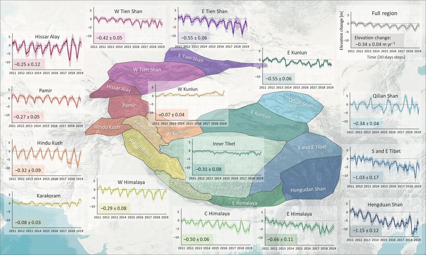
The Cryosphere, 15, 1845–1862, 2021 https://doi.org/10.5194/tc-15-1845-2021L. Jakob et al.: Ice loss in High Mountain Asia and the Gulf of Alaska between 2010 and 2019 1857 Figure 9. Gulf of Alaska (GoA) monthly elevation change time series on a sub-regional level. The coloured lines display the time series with the uncertainty envelope (y axis: elevation change [m]; x axis: time [30 d steps]). The numbers describe the elevation change with uncertainties in m yr−1 . Figure 10. Gulf of Alaska (GoA) monthly surface elevation change time series with uncertainty envelopes at different elevation bands aggregated on the RGI 6.0 second-order regions. The different colours represent the elevation bands (> 3000, 2000–3000, 1000–2000, 0– 2000 m). Elias mountains − which are also the areas where the low- the same altitude. These findings indicate a propagation of ering of mean surface elevations after 2013–2014 has been thinning upstream compared to the time period 1962–2006. most pronounced (see Figs. 9, S3). In comparison to the In contrast, whilst on the Alaska Peninsula elevation changes study by Berthier et al. (2010), which is based on sequen- have increased at lower altitudes, the limit of the thinning tial digital elevation models over the time period from 1962 area has stayed the same since the survey time period of to 2006, we observe similar elevation changes at the low- Berthier et al. (2010). est altitudes but less steep gradients in sub-regions along the In the western Chugach Mountains, Alaska Range, and east coast (Fig. 11, Table S2). This is particularly pronounced Alaska Peninsula, we observe a decrease in thinning rates in the Saint Elias Mountains, where Berthier et al. (2010) towards the lowest elevations of these sub-regions, which show near-balance at around 1000 m a.s.l., whilst our esti- can be attributed to the effect of debris cover and the tem- mates suggest a surface elevation change of −1.5 m yr−1 at poral evolution of glacier extent during the study period, one https://doi.org/10.5194/tc-15-1845-2021 The Cryosphere, 15, 1845–1862, 2021
1858 L. Jakob et al.: Ice loss in High Mountain Asia and the Gulf of Alaska between 2010 and 2019
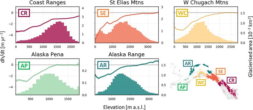
Figure 11. Altitudinal distribution of elevation changes and glacier hypsometry functions in the Gulf of Alaska (GoA) in RGI 6.0 sub-regions
between 2010 and 2019. The lines show elevation change rates with uncertainty envelopes plotted against 100 m elevation bands (left y axis).
The bars display the glacier hypsometry (right y axis).
ries of elevation change, exploiting CryoSat’s high tempo-
ral repeat, to reveal seasonal and multiannual variation in
rates of glaciers’ thinning. We find that between 2010 and
2019, HMA has lost mass at a rate of 28.0 ± 3.0 Gt yr−1
(0.29 ± 0.03 m w.e. yr−1 ), and the GoA region has lost mass
at a rate of 76.3 ± 5.7 Gt yr−1 (0.89 ± 0.07 m w.e. yr−1 ),
for a sea level contribution of 0.078 ± 0.008 mm yr−1
(0.051 ± 0.006 mm yr−1 from exorheic basins) and 0.211 ±
0.016 mm yr−1 , respectively, for HMA and the GoA. Both re-
gions have lost over 4 % of their respective ice volume during
the 9-year study period. These estimates are broadly consis-
tent with the range of estimates generated by previous studies
and highlight the significant discrepancies that remain in the
assessments of mass loss for these two regions.
In HMA we find the most negative surface elevation trends
Figure 12. Gulf of Alaska (GoA) specific mass balance trends, ag- in the Nyainqêntanglha Mountains, Hengduan Shan, the east-
gregated on the sub-regions by Berthier et al. (2010). The figure ern Himalayan range, and the Tien Shan and slightly posi-
compares our results (July 2010 to July 2019) to the estimates of tive and near-balance trends in the Kunlun and Karakoram
Berthier et al. (2010), covering the time period 1962 to 2006. ranges, known as the “Karakoram anomaly”. The monthly
time series of this paper reflect the sensitivity of glaciers in
HMA to meteorological patterns and changes and empha-
of the limitations of using static glacier masks. This charac- sizes that the temporal variability in glaciers in High Moun-
teristic has been observed, although more pronounced and tain Asia varies spatially. We show sustained multiannual
across all sub-regions, by Berthier et al. (2010) and Arendt et trends across almost all of the sub-regions until 2015–2016
al. (2002). and decreased loss or even mass gain from 2016 to 2017 on-
wards.
Negative mass trends are also observed in all of the sub-
5 Conclusion regions in the GoA region, with the largest mass losses in the
Coast Ranges and the Saint Elias Mountains. The GoA time
We exploit CryoSat-2 interferometric-swath-processed data series reveal an increased mass loss from 2013–2014, most
from 2010 to 2019, with a total of 33 million elevation pronounced in sub-regions along the south-central and south-
observations, to generate new and independent mass bal- east coast (Saint Elias Mountains, Chugach Mountains, and
ance estimates for two mountain regions: the Gulf of Alaska Coast Ranges) at lower elevations. This mass loss acceler-
(GoA) and High Mountain Asia (HMA). We also generate ation is linked with the change from a negative to a pos-
observations at the sub-regional level and extract elevation- itive Pacific Decadal Oscillation (PDO), which resulted in
dependent thinning rates, revealing contrasting mass loss increased temperatures. In general, our time series not only
across sub-regions. Finally, we extract monthly time se- display the sensitivity of glaciers to climatic conditions and
The Cryosphere, 15, 1845–1862, 2021 https://doi.org/10.5194/tc-15-1845-2021You can also read