Spatiotemporal Analysis of Water Resources in the Haridwar Region of Uttarakhand, India - MDPI
←
→
Page content transcription
If your browser does not render page correctly, please read the page content below
sustainability

Article
Spatiotemporal Analysis of Water Resources in the
Haridwar Region of Uttarakhand, India
Shray Pathak 1, * , Chandra Shekhar Prasad Ojha 2 , Rahul Dev Garg 2 , Min Liu 1 ,
Daniel Jato-Espino 3, * and Rajendra Prasad Singh 4
 1    Key Laboratory of Geographical Information Sciences, Ministry of Education, and School of
      Geographic Sciences, Institute of Eco-Chongming, East China Normal University, Shanghai 200241, China;
      mliu@geo.ecnu.edu.cn
 2    Department of Civil Engineering, Indian Institute of Technology Roorkee, Uttarakhand 247667, India;
      c.ojha@ce.iitr.ac.in (C.S.P.O.); rdgarg@ce.iitr.ac.in (R.D.G.)
 3    Department of Transport and Projects and Processes Technology, Universidad de Cantabria,
      Av. de los Castros 46, 39005 Santander, Spain
 4    School of Civil Engineering, Southeast University, Nanjing 210096, China; rajupsc@seu.edu.cn
 *    Correspondence: shraypathak@gmail.com (S.P.); daniel.jato@unican.es (D.J.-E.)

 Received: 19 August 2020; Accepted: 10 October 2020; Published: 14 October 2020

 Abstract: Watershed management plays a dynamic role in water resource engineering. Estimating
 surface runoff is an essential process of hydrology, since understanding the fundamental relationship
 between rainfall and runoff is useful for sustainable water resource management. To facilitate the
 assessment of this process, the Natural Resource Conservation Service-Curve Number (NRCS-CN)
 and Geographic Information Systems (GIS) were integrated. Furthermore, land use and soil maps
 were incorporated to estimate the temporal variability in surface runoff potential. The present study
 was performed on the Haridwar city, Uttarakhand, India for the years 1995, 2010 and 2018. In a
 context of climate change, the spatiotemporal analysis of hydro meteorological parameters is essential
 for estimating water availability. The study suggested that runoff increased approximately 48% from
 1995 to 2010 and decreased nearly 71% from 2010 to 2018. In turn, the weighted curve number was
 found to be 69.24, 70.96 and 71.24 for 1995, 2010 and 2018, respectively. Additionally, a validation
 process with an annual water yield model was carried out to understand spatiotemporal variations
 and similarities. The study recommends adopting water harvesting techniques and strategies to
 fulfill regional water demands, since effective and sustainable approaches like these may assist in the
 simultaneous mitigation of disasters such as floods and droughts.

 Keywords:      water resources                management;   urban   sprawl;   rainfall-runoff    modeling;
 spatiotemporal variation

1. Introduction
     Water assets are the most essential renewable resources required by inhabitants in all forms.
Thus, the consumption of water resources needs an effective decision planning for handling both its
quality and quantity by considering its spatiotemporal variations. Land use and land cover (LULC)
classification describes the role of human beings in affecting the land-cover patterns with time, which
ultimately reflects the amount of surface runoff that different types of surface can deal with [1].
     Cities experience high surface flows when the ratio of rainfall to infiltration rate is higher [2].
The amount of runoff generated depends upon LULC, soil properties, topography, slope, vegetation
cover and atmospheric conditions [3–8]. The estimation and storage of stormwater is an essential
component in the hydrological cycle to maintain the equilibrium in the city. Estimating surface

Sustainability 2020, 12, 8449; doi:10.3390/su12208449                      www.mdpi.com/journal/sustainability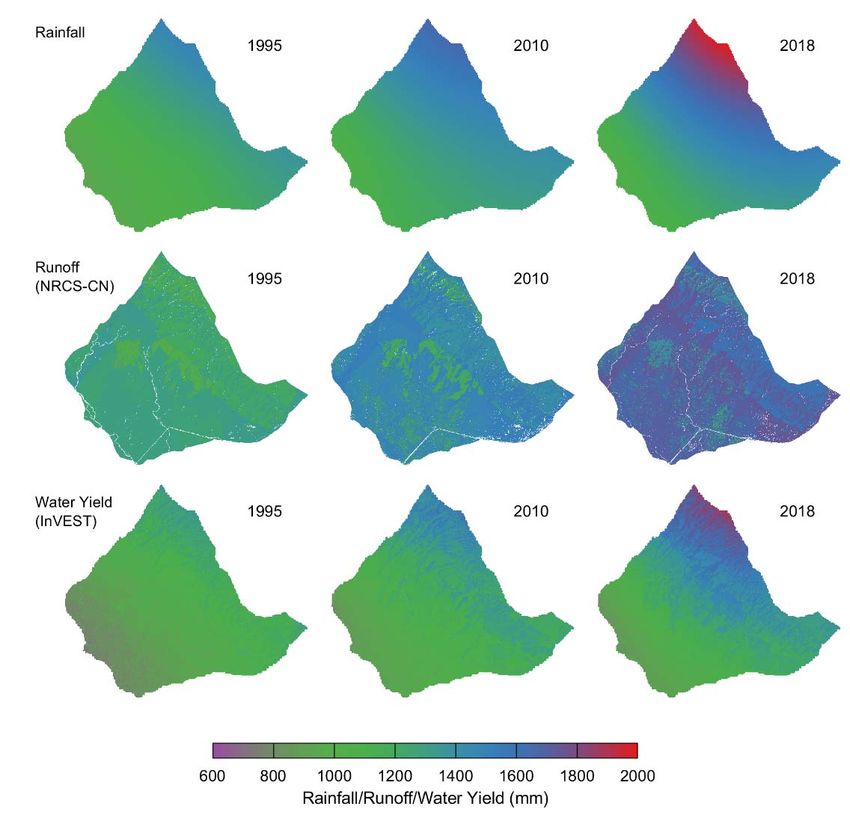
Sustainability 2020, 12, 8449                                                                        2 of 17

runoff is essential and plays an important role in hydrological engineering, modeling, and its related
applications such as water balance calculation and flood design [9–11]. However, accounting for the
spatiotemporal variability of runoff is complex, as it is governed by different hydrological parameters.
      The National Resources Conservation Service-Curve Number (NRCS-CN) method, commonly
known as the Soil Conservation Service-Curve Number (SCS-CN) method, was developed by the
National Resource Conservation Service United State Department of Agriculture (USDA) in 1976.
It is a reliable and straightforward method for estimating surface runoff from rainfall by obtaining
curve number maps [12–19]. This approach is a direct function of the composite curve number (CN)
to estimate the fraction of rainfall that flows as surface runoff [20,21]. High-resolution images help
in computing the CN spatially to further estimate water flows within cities [22–27]. The role of the
NRCS-CN model, including its concept, application, capabilities and limitations are clearly described
in the scientific literature [28,29].
      The conventional approach to compute CN for any catchment is to use available curves and
tables, which is tedious and time consuming [9,20,30]. However, the implementation of this technique
at the gridded scale by using GIS software becomes easier and takes less time [31–34]. The output
generated in the gridded format is more reliable, provides detailed assessment and helps in developing
strategic decision planning [35–40]. Globally, many studies have been performed using GIS techniques
to simulate surface runoff [14,41–46]. A research focused on the Bebas river in Madha Pradesh
yielded strong correlations between measured and simulated runoff depths using a GIS-based SCS-CN
model [47]. Furthermore, the CN was applied to the Indian conditions using SCS-CN and GIS
techniques to estimate spatial hydrological parameters and temporal variables [48]. In another study,
GIS and remote sensing are concluded to be powerful tools for estimating runoff depth generation
in the geo-hydrological environment [49]. Additionally, eight different models were combined with
the SCS-CN model to calculate the accuracy of surface runoff depth estimates for 15 watersheds in
Korea [50]. This technique was also utilized to identify and artificially recharge water harvesting
structures [51–54].
      Furthermore, similar parameters are required by other hydrological models such as Natural
Capital Project’s Integrated Valuation of Ecosystem Services and Tradeoffs model (InVEST) to estimate
spatial water yield [55,56]. This model is developed based on the Budyko theory and consists
of different tools for ecosystem assessment. To understand the role of meteorological parameters,
the InVEST model has been applied both for extreme dry and wet conditions [57]. Additionally,
it has been used to study different scenarios of urban sprawl and climate change in the watersheds
of northwestern Oregon state [58], as well as to quantify sediment retention, water yield, carbon
sequestration, and habitat quality under future land-use scenarios [59]. Pathak et al. [60] analyzed
and validated the model for different watersheds varying in topographic characteristics. In urban
areas, a major issue is to identify and locate suitable sites by considering socio-economic aspects
of suitability [61]. Strategized policies are based on short-term scenarios and have low potential to
handle extreme scenarios. The advancements in GIS tools have the capability to locate suitable sites
for water harvesting and implement conservation practices [62]. Integrated geospatial technologies
are essential to obtain updated information on LULC, soil texture, hydrologic soil groups and spatial
rainfall variation to estimate surface runoff [63–68]. Calibration and validation of surface runoff models
are very important to minimize uncertainty in the observed modeling inputs [69]. Additionally, public
participation is involved through crowdsourcing along with stakeholders and water planners for an
effective decision-making process [70].
      Furthermore, an effective decision planning at a city scale is based on analyzing both the spatial and
temporal variability of the water potential of the region. Long-term planning requires the evaluation
of the spatiotemporal trend of surface runoff corresponding to rainfall. In this context, the analysis
of variations in LULC is essential. If a stronghold is established on previous records, this kind of
assessment could contribute to improving decision-making processes related to the management of
water related disasters. Thus, the objective of the present study is twofold: to observe the effect of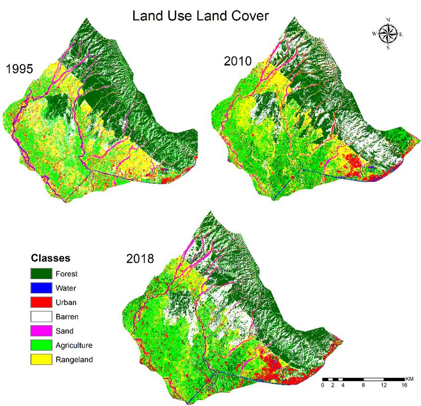
Sustainability 2020, 12, 8449                                                                              3 of 17
Sustainability 2020, 12, x FOR PEER REVIEW                                                                  3 of 17

the spatiotemporal
 number               variations
           and to ascertain       of rainfall on and
                              the applicability  surface  runoff dueoftoincorporating
                                                      effectiveness      changes in thethe
                                                                                         curve numbermethod
                                                                                            NRCS‐CN      and to
ascertain   the applicability  and  effectiveness  of incorporating  the  NRCS-CN     method   into
 into geospatial tools. The study also evaluates the temporal effect of anthropogenic activities on geospatial
tools. The
 spatial     studyrunoff
         surface   also evaluates  the temporal
                         for the study            effect of anthropogenic
                                        region, Haridwar,                  activities
                                                             India. This will         on spatial
                                                                              assist water       surface
                                                                                           planners      runoff
                                                                                                     to identify
for the  study  region, Haridwar,    India.  This will  assist water planners   to identify suitable
 suitable zones for artificially recharge aquifers or water harvesting structures in the region.      zones for
artificially recharge aquifers or water harvesting structures in the region.
 2. Study Area
2. Study Area
      The study area considered is Haridwar city, Uttarakhand, India. It is one of the seven holiest
      The study area considered is Haridwar city, Uttarakhand, India. It is one of the seven holiest places
 places to Hindus. Hence, it is essential to estimate water yield availability and the effect of
to Hindus. Hence, it is essential to estimate water yield availability and the effect of anthropogenic
 anthropogenic activities, since the area is visited by millions of devotees worldwide. Consequently,
activities, since the area is visited by millions of devotees worldwide. Consequently, the analysis
 the analysis was performed to understand the temporal impact on the landscape of the study region,
was performed to understand the temporal impact on the landscape of the study region, which
 which is represented in Figure 1. The geophysical characterization of the study region is described in
is represented in Figure 1. The geophysical characterization of the study region is described in
 subsequent sub‐sections.
subsequent sub-sections.

                           Figure 1. Geographical representation of the Haridwar city, India.
                           Figure 1. Geographical representation of the Haridwar city, India.
      The Haridwar district is extended up to an area of about 2400 sq. km and located in the southwest
part ofThe
         theHaridwar
             Uttarakhanddistrict
                           state,isIndia.
                                     extended    up to
                                          Haridwar      anthe
                                                     is at  area  of about
                                                               height  of 3162400  sq. km
                                                                              m above       and located
                                                                                        the mean  sea levelinand
                                                                                                               the
 southwest    part of the Uttarakhand     state, India. Haridwar    is at the height of 316  m above
lies within the North and Northeast of the Shivalik hills and the Ganges River in the South. The whole the  mean
 sea level
area        and lies
      is divided  intowithin the North
                       four parts:        and Northeast
                                     mountainous    region,ofupper
                                                              the Shivalik
                                                                     bajada,hills and
                                                                              lower    the Ganges
                                                                                     bajada         River plain.
                                                                                             and alluvial   in the
 South. The whole area is divided into four parts: mountainous region, upper bajada, lower bajada
Major land-use classes in the study area are urban, agricultural, forest and barren land. Most of the
 and alluvial plain. Major land‐use classes in the study area are urban, agricultural, forest and barren
study area (35% approximately) is forest. Moderate growth is observed, especially in roads and urban
 land. Most of the study area (35% approximately) is forest. Moderate growth is observed, especially
classes, as observed in 2018.
 in roads and urban classes, as observed in 2018.
      The study of climate data indicated that this area corresponds to a moderate subtropical humid
       The study of climate data indicated that this area corresponds to a moderate subtropical humid
region with a temperature drop in March (29.1 ◦ C) that begins to rise until reaching its maximum in May
 region with a temperature drop in March (29.1 °C) that begins to rise until reaching its maximum in
(39.2 ◦ C). In mid-June, when the monsoon starts, the temperature starts falling. It is within the range
 May (39.2 °C). In mid‐June, when the monsoon starts, the temperature starts falling. It is within the
from 10.5 ◦ C to 6.1 ◦ C from November to February during the winter season. Annual rainfall is about
 range from 10.5 °C to 6.1 °C from November to February during the winter season. Annual rainfall
1200 mm. About 84% of this figure falls within the monsoon season and the rest are in non-monsoon
 is about 1200 mm. About 84% of this figure falls within the monsoon season and the rest are in non‐
periods. Maximum precipitation occurs in the Himalayan foothills and decreases gradually while
 monsoon periods. Maximum precipitation occurs in the Himalayan foothills and decreases gradually
 while shifting towards the south. In the summer, the mean monthly wind speed is highest in May
 and June, corresponding to 7.4 and 7.2 km/h, and it decreases to its minimum in October (2.6 km/h).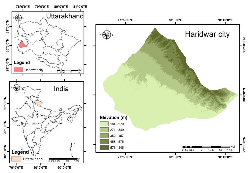
2018 year, 8 years of past record is considered for evaluation. Thus, the preparation of input variables
      to estimate the spatial variation in runoff in different years and understand their correlation is
      described in subsequent subsections.

      3.1. Land Use Land Cover
Sustainability 2020, 12, 8449                                                                                   4 of 17
           Landsat images were acquired from the United States Geological Survey (USGS) and clipped
      according to the extent of the study area for the years 1995, 2010, and 2018. Preprocessing analyses
shifting towards
      were          the on
            performed    south.
                            theseInimages
                                    the summer,   the
                                          using the   mean monthlysoftware.
                                                    ERDAS‐Imagine       wind speed   is highest
                                                                                The LULC          in May and
                                                                                             classification was June,
corresponding    to  7.4  and 7.2  km/h,  and it decreases  to its minimum    in October   (2.6  km/h).
      achieved by adopting the nearest neighbor classifier and an object‐based image analysis approach.
      As a result, the study area was classified into seven classes, i.e., water, forest, sand, eroded land,
3. Materials   and Methods
      urban, rangeland    and agriculture with a spatial resolution of 30 m. The classification was validated
      using ground truth points and Google Earth images.
     The flowchart corresponding to the methodology to estimate spatial surface runoff is illustrated
in Figure    2. Depth
      3.2. Soil  Different inputs to the models were prepared in raster format to analyze spatial and
                      and Texture
temporal zonal effects. The study has considered temporal variation since 1981, by performing analysis
            The soil map was acquired from the National Bureau of soil survey and land‐use planning
for three years i.e., 1995 (1981–1995), 2010 (1996–2010), and 2018 (2011–18). The analysis for the
      (NBSSLUP) at a scale of 1:250,000. In grid format, the resolution was resampled from 1200 m to 30 m
years 1995 and 2010 have considered and averaged the past 15 years of datasets whereas for the 2018
      to achieve the same spatial resolution of LULC using ArcGIS. Different information about the soil is
year, available
       8 years ofin past record
                    the map  suchis as
                                    considered
                                       soil depth,for evaluation.
                                                   slope, percentageThus, the preparation
                                                                     of carbon              of input
                                                                               content, texture,      variables to
                                                                                                 temperature,
estimate   the  spatial variation  in  runoff in different years  and understand   their  correlation is described
      erosion, drainage, and mineralogy. The required data, viz. soil depth and texture, was transformed
in subsequent     subsections.
      into the raster format to perform as an input in the hydrological model.

             Figure
      Figure 2.     2. Flowchart
                Flowchart  of the of the methodology
                                  methodology         forNatural
                                                for the   the Natural Resources
                                                                 Resources       Conservation
                                                                            Conservation      Service‐CurveNumber
                                                                                            Service-Curve
                                 Number   (NRCS‐CN)
      (NRCS-CN) model (Source: Pathak et al. [71]).    model  (Source: Pathak et al. [71]).

3.1. Land Use Land Cover
     Landsat images were acquired from the United States Geological Survey (USGS) and clipped
according to the extent of the study area for the years 1995, 2010, and 2018. Preprocessing analyses
were performed on these images using the ERDAS-Imagine software. The LULC classification was
achieved by adopting the nearest neighbor classifier and an object-based image analysis approach.
As a result, the study area was classified into seven classes, i.e., water, forest, sand, eroded land, urban,
rangeland and agriculture with a spatial resolution of 30 m. The classification was validated using
ground truth points and Google Earth images.

3.2. Soil Depth and Texture
     The soil map was acquired from the National Bureau of soil survey and land-use planning
(NBSSLUP) at a scale of 1:250,000. In grid format, the resolution was resampled from 1200 m to 30 m
to achieve the same spatial resolution of LULC using ArcGIS. Different information about the soil is
available in the map such as soil depth, slope, percentage of carbon content, texture, temperature,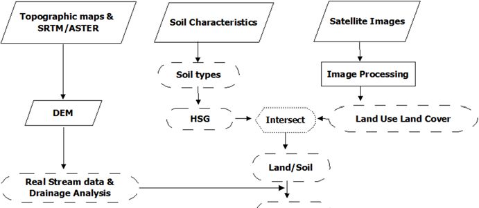
Sustainability 2020, 12, 8449                                                                         5 of 17

erosion, drainage, and mineralogy. The required data, viz. soil depth and texture, was transformed
into the raster format to perform as an input in the hydrological model.
     According to its characteristics, soil is classified into four hydrologic soil groups (HSG), i.e., A, B,
C and D. The groups are assigned according to the runoff potential and infiltration capacity of the soil.
Groups A to D have high to low infiltration capacity and low to high runoff potential. This parameter
assists in computing the composite CN and estimating the fraction of rainfall that flows as surface
runoff within a city [72].

3.3. Precipitation and Temperature
     The daily series of temperature and precipitation were collected in gridded format with a spatial
resolution of 1◦ and 0.25◦ , respectively, from the Indian Meteorological Department (IMD). The dataset
used in the study is from 1981 to 2018 [73–76].

3.4. Surface Runoff
      A combination of the NRCS-CN method with GIS tools was applied to estimate spatial runoff.
The NRCS-CN method considers some readily available tables and curves and is based upon a simple
empirical formula to obtain surface runoff. The curve number (CN) is an important parameter that
influences the estimation of surface runoff. High values of CN represent high amounts of surface
runoff and low infiltration capacity of the soil, and vice versa. The CN, which is a function of land use,
soil property and slope, was obtained using LULC and soil maps [77].

                                     (P − Ia )2
                                Q=              for P > Ia Q = 0 for P ≤ Ia                              (1)
                                     P − Ia + S

where Q is direct runoff, P represents total rainfall, S is the potential maximum retention, and Ia is the
initial abstraction. Ia is a function of S that can be expressed as

                                                  Ia = λS                                                (2)

Equation (1) becomes,
                                                   (P − λS)2
                                            Q=                                                           (3)
                                                  P + (1 − λ)S
    Here, S can be estimated from the P–Q data for a constant value of Ia (0.2 S), and represented in
terms of CN using Equation (4).
                                            25400
                                        S=         − 254                                          (4)
                                             CN
    The curve number is obtained from three variables: land use land cover, hydrologic soil group
(HSG), and antecedent moisture condition (AMC) [72]. Hence, the weighted curve number for the
study region can be determined by the following formula.
                                                    P
                                                        CNi × Ai
                                           CNw =                                                         (5)
                                                         A
where CNw represents the weighted curve number, A is the total area, CNi is the curve number of
sub-catchment i, where sub-catchments (or sub-areas) ranges from 1 to any number N, Ai is the area of
sub-catchment i, and N is the total number of sub-catchments in a watershed.

3.5. Annual Water Yield
     The InVEST model has the potential to capture the alteration in the flows due to changes in the
ecosystem [60]. This model entirely works according to an empirical function derived from the Budyko
framework, which provides the ratio of potential evapotranspiration (PET) to actual evapotranspiration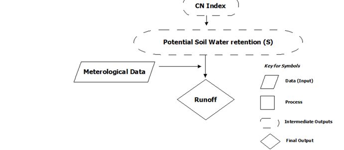
Sustainability 2020, 12, 8449                                                                       6 of 17

(AET) [78]. The InVEST model captures the spatial variability in precipitation, vegetation, PET, and soil
depth to estimate spatial changes in the LULC. The model works on grid format and estimates the
heterogeneity in the parameters (LULC, precipitation, temperature, HSG, etc.) affecting the water
flows. The spatial water yield is estimated annually for each land use class as follows:
                                                                !
                                                        AET (x)
                                            Y (x) = 1 −           × P (x)                              (6)
                                                         P (x)

where, P(x) represents the spatial annual precipitation and AET(x) refers to the actual annual
evapotranspiration at each pixel x.
     Precipitation and PET determines the mean AET of the watershed. Some of the watershed
characteristics, i.e., topography, soil, etc., plays a secondary role. The index of dryness refers to the
ratio of annual PET to precipitation to estimate the annual AET.
                                                                      #( 1 )
                                                               PET (x) ω
                                                           "
                                     AET (x)      PET (x)
                                             = 1+         − 1+                                         (7)
                                      P (x)        P (x)        P (x)

where ω(x) is a non-physical parameter that represents the natural climatic soil properties and PET at
each pixel. PET is further estimated by the following expression.

                                             PET (x) = Kc (x) × ETo (x)                                (8)

where Kc(x) represents the vegetation evapotranspiration coefficient, which is a function of the LULC
characteristics [79]. Furthermore, ET0 is the annual reference evapotranspiration, which is determined
on the basis of alfalfa grass grown as Equation (11). In addition, ω(x) is an empirical parameter
determined by Donohue et al. [80] as follows.

                                                           AWC (x)
                                             ω (x) = z ×           + 1.25                              (9)
                                                            P (x)

where z is the seasonality factor, the value of which varies from 1 to 30. Further, AWC is a function of
the volumetric plant available water content (mm) and is determined through Equation (10).

                        AWC (x) = Min. (Root depth, Restricting layer depth) × PAWC                  (10)

      The maximum depth in the soil up to which the roots can penetrate is referred to as root restricting
layer depth. Additionally, the depth up to which 95% of the root biomass occurs is defined as root depth.
PAWC is the plant available water content, which generally stands for the difference between field
capacity and wilting point. ETo is estimated by the modified Hargreaves method, which is a function
of average daily temperature (Tavg ), temperature range (TD), ETo , and extraterrestrial radiation (RA).
Tavg (◦ C), is the mean of the mean daily maximum and mean daily minimum temperatures, and TD
(◦ C) represents the temperature range obtained as the difference between the mean daily maximum
and daily minimum temperatures.

                        ETo = 0.0013 × 0.408 × RA × Tavg + 17.0 × (TD − 0.0123 × P)0.76

                                                                                                     (11)

      To estimate RA, the expression is given as follows:

                                24(60)
                      RA =             × Gsc × dr × [ws sin(ϕ) sin(δ) + cos(ϕ) cos(δ) sin(ws )]      (12)
                                  π
Sustainability 2020, 12, 8449 7 of 17
where dr is the inverse relative distance Earth–Sun, RA is extraterrestrial radiation [MJm−2 d−1 ], Gsc is
a solar constant equal to 0.0820 MJm−2 min−1 , δ is solar declination (rad), ws is sunset hour angle (rad)
and ϕ is latitude (rad).
In the present study, this approach was utilized to validate the CN based water yield estimates.
The InVEST model was applied to understand the spatiotemporal trend of annual water yield with
runoff. Moreover, it enables validating both the range and the spatial variation of temporal runoff for
the selected years. Further, it provides a second base to deploy decision planning based on spatial
Sustainability 2020, 12, x FOR PEER REVIEW 7 of 17
water availability within the study area.
4. Results and Discussion
4. Results and Discussion
4.1. Supervised
4.1. Supervised Classification
Classification
The LULC
The LULC classification
classification for
for the
thestudy
studyperiod
periodwas
wasobtained
obtainedusing
using supervised classification,
supervised as
classification,
represented in Figure 3. The study area was divided into seven classes, i.e., forest, water, sand,
as represented in Figure 3. The study area was divided into seven classes, i.e., forest, water, sand, eroded
land, urban,
eroded land, rangeland and agriculture.
urban, rangeland Table 1 reveals
and agriculture. Table 1 the percentage
reveals area covered
the percentage by each class
area covered for
by each
the years 1995, 2010 and 2018.
class for the years 1995, 2010 and 2018.
Figure 3. Land Use/Land Cover (LULC)
Figure 3. (LULC) map
map of
of the
the study
study area
area for
for the
the years
years 1995,
1995, 2010
2010 and
and 2018.
2018.
Table 1. Classification of land-use classes for the years 1995, 2010 and 2018.
Table 1. Classification of land‐use classes for the years 1995, 2010 and 2018.
Class Class Percentage (1995)
Percentage (1995) Percentage
Percentage (2010)PercentagePercentage
(2010) (2018) (2018)
Forest Forest 29.5729.57 30.68
30.68 28.12 28.12
Water Water 1.37 1.37 1.431.43 1.51 1.51
Eroded landEroded land 18.3218.32 18.11
18.11 21.26 21.26
Sand Sand 3.73 3.73 2.212.21 2.38 2.38
Urban Urban 5.5 5.5 6.3 6.3 8.71 8.71
Rangeland 20.34 19.76 11.23
Rangeland 20.34 19.76 11.23
Agriculture 20.02 21.53 26.79
Agriculture 20.02 21.53 26.79
From Table 1, it is understood that a large part of the study area is covered under forest, which
is approximately 30% of the total area (254 sq. km). The upper Siwalik region is covered with forest
and some built‐up areas that include urban forests. Agriculture and rangeland extends to
approximately 40%, as agriculture is a major occupation in this region. Water bodies account for
approximately 1.4% of the total area since 1995. Most of this water is transmitted through the canalSustainability 2020, 12, 8449 8 of 17
From Table 1, it is understood that a large part of the study area is covered under forest, which is
approximately 30% of the total area (254 sq. km). The upper Siwalik region is covered with forest and
some built-up areas that include urban forests. Agriculture and rangeland extends to approximately
40%, as agriculture is a major occupation in this region. Water bodies account for approximately 1.4%
of the total area since 1995. Most of this water is transmitted through the canal in the study area,
with some small ponds and lakes situated near the residential area. The flashy stream contains water
only in the monsoon season. Eroded land is formed due to the erosion of the surface caused by high
discharge. The slopes are steep (more than 12%) and streams contain large flows in the monsoon
season. To verify the accuracy of this supervised classification, an accuracy assessment was performed
as tabulated in Table 2. User accuracy corresponds to the error of commission whereas producer
accuracy defines the error of omission in the LULC classification. In other words, user accuracy is the
ratio of the number of pixels correctly identified to the number of pixels claimed to be in the respective
maps class. The producer accuracy is the ratio of the number of pixels correctly identified in reference
plots to the number actually in that reference class. Thus, user and producer accuracy were computed
for each class of the study area as described in Table 2.
Table 2. Accuracy assessment of supervised classification for the years 1995, 2010 and 2018.
1995 2010 2018
LULC Classes Producer User Producer User Producer User
Accuracy Accuracy Accuracy Accuracy Accuracy Accuracy
(%) (%) (%) (%) (%) (%)
Forest 74.35 82.85 76.38 83.65 77.52 83.36
Wasteland 74.36 82.85 77.36 82.36 74.25 82.14
Rangeland 78.94 85.71 77.69 86.32 79.69 86.31
Agriculture 79.82 85.71 81.23 86.36 79.36 85.10
Built up 84.84 80.00 85.36 78.36 84.69 81.23
Sand 72.97 77.84 73.25 79.32 73.36 79.25
Water 84.00 60.00 85.36 72.00 85.00 65.00
4.2. Trend Analysis of Land Cover Classes
The trend analysis chart is shown in Figure 4. It shows that the forest area reduced from 29.57%
(250.46 sq. km) in 1995 to 28.12% (238.176 sq. km) in 2018. The change in forest area is not significant
as compared to the increased urban area because of the policies strategized by the government to
protect forest. Water class has remained constant since 1995, because most of the water demand is
met by the canal. Very little change is observed in the water class as the water flows in the flashy
streams. Built-up area increased from 5.5%, (46.58 sq. km) in 1995 to 8.71%, (73.77 sq. km) in 2018.
Most of the urbanization is in the lower Siwalik and the plain region. Total cultivable land, which was
approximately 40% in 1995, also decreased and became 38% in the year 2018, representing urbanization
as directly proportional to cultivation. The eroded land increased by approximately 3% of the area
directing the influence of flashy streams and anthropogenic activities in the area. Moreover, the region
experienced high sediment loads, which makes it more vulnerable to flood risk. Thus, suitable low
impact development (LID) techniques should be implemented at specified zones to mitigate potential
negative impacts and prevent socio-economic loss.was approximately 40% in 1995, also decreased and became 38% in the year 2018, representing
urbanization as directly proportional to cultivation. The eroded land increased by approximately 3%
of the area directing the influence of flashy streams and anthropogenic activities in the area.
Moreover, the region experienced high sediment loads, which makes it more vulnerable to flood risk.
Thus, suitable low impact development (LID) techniques should be implemented at specified zones
Sustainability 2020, 12, 8449 9 of 17
to mitigate potential negative impacts and prevent socio‐economic loss.
Sustainability 2020, 12, x FOR PEER REVIEW 9 of 17
Figure 4.
Figure Trend chart
4. Trend chart of
of LULC
LULC for
for the
the study
study area
area from
from 1995
1995 to
to 2018.
2018.
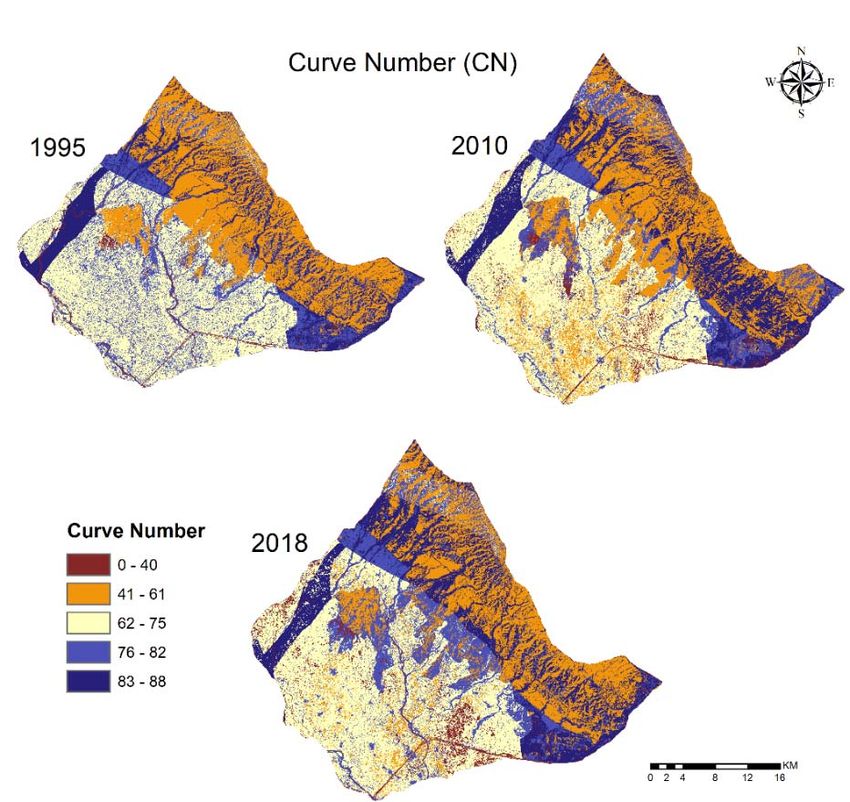
4.3. Curve Number Analysis
4.3. Curve Number Analysis
Once the raster map was prepared for the soil and LULC, the maps were integrated into the
Once environment
ArcGIS the raster map was prepared
to create the curve for the soil
number map.and LULC,
Hence, thethe maps
curve weremaps
number integrated intoforthe
obtained
ArcGIS environment to create the curve number map. Hence, the curve number maps
the study area are represented in Figure 5. The higher value of curve number defines the higher obtained for the
study areafor
runoff are represented
that particular in Figure
zone 5. The
and vice higher
versa. Thevalue ofportray
results curve number definesofthe
a clear picture thehigher runoff
zones that arefor
thatexperiencing
particular zone and vice versa. The results portray a clear picture of the zones that are
high surface runoff. Thus, to handle drought and flooding situations, water harvestingexperiencing
high surfaceshould
schemes runoff.beThus, to handleindrought
implemented and flooding
these specific situations,
areas having water harvesting
an abundant amount of schemes should
surface water
be availability.
implemented Inin these
this specific
scenario, theareas having
zones havinganhigher
abundant amount
CN value of surface
represents water availability.
potential suitable sitesInfor
this
water harvesting.
scenario, the zones having higher CN value represents potential suitable sites for water harvesting.
Figure5.5.Curve
Figure Curve number
number map of
of the
the study
studyarea.
area.
4.4. Variation in Area Ratio
The curve number is a function of the LULC and soil property of the area. Figure 6 shows the
spatial distribution of the CN during the years 1995, 2010 and 2018. Area ratio represents the ratio of
a particular land covered with a specific number of CN values to the total area. It is understood fromSustainability 2020, 12, 8449 10 of 17
4.4. Variation in Area Ratio
The curve number is a function of the LULC and soil property of the area. Figure 6 shows the
spatial distribution of the CN during the years 1995, 2010 and 2018. Area ratio represents the ratio of a
particular land covered with a specific number of CN values to the total area. It is understood from
Figure 6 that the CN is increasing from 1995 to 2018. The initial range of CN (26–61) belongs to the
forest area, which is decreasing from 1995 to 2018. The agriculture and crop areas are also reduced,
and the maximum deviation in the CN is in the range of 83–87, which belongs to wasteland and built
up area. A decrease in forest and cultivated land and an increase in wasteland and built-up area
Sustainability 2020, 12, x FOR PEER REVIEW
are
10 of 17
observed in the city due to the effect of urban sprawl.
Figure 6.
Figure Variation of
6. Variation of area
area ratio
ratio with
with Curve
Curve Number
Number for
for the
the years
years 1995,
1995, 2010
2010 and
and 2018.
2018.
4.5. Runoff Analysis
4.5. Runoff Analysis
Monthly runoff was estimated for the study area by providing rainfall data as an input to the
Monthly runoff was estimated for the study area by providing rainfall data as an input to the
NRCS-CN method, as represented in Figure 7. For the year 1995, maximum rainfall was observed in
NRCS‐CN method, as represented in Figure 7. For the year 1995, maximum rainfall was observed in
August, which corresponds to AMC III condition and a maximum amount of runoff for this period.
August, which corresponds to AMC III condition and a maximum amount of runoff for this period.
About 85% of the yearly rainfall is observed in July to August, contributing to maximum runoff in
About 85% of the yearly rainfall is observed in July to August, contributing to maximum runoff in
these months. AMC I condition exists for the rest of the months, as they received less rainfall and
these months. AMC I condition exists for the rest of the months, as they received less rainfall and
thus resulted in a lower amount of runoff. Thus, an adjustment table was referred to select the curve
thus resulted in a lower amount of runoff. Thus, an adjustment table was referred to select the curve
number corresponding to different soil moisture conditions [81].
number corresponding to different soil moisture conditions [81].
For the year 2010, the area receives a lower amount of rainfall in the non-monsoon period, whilst
For the year 2010, the area receives a lower amount of rainfall in the non‐monsoon period, whilst
approximately 87% of total rainfall occurs during the monsoon period. The AMC III condition is
approximately 87% of total rainfall occurs during the monsoon period. The AMC III condition is
applicable for the monsoon region, thereby causing a higher amount of runoff in this period. Some of
applicable for the monsoon region, thereby causing a higher amount of runoff in this period. Some
the rainfall is observed in the winter season due to the western disturbances, but runoff is nearly zero
of the rainfall is observed in the winter season due to the western disturbances, but runoff is nearly
because of the non-saturation condition of the soil. As for 2018, rainfall is very low as compared to
zero because of the non‐saturation condition of the soil. As for 2018, rainfall is very low as compared
previous years. Because of the lesser rainfall in the area, the AMC II condition is applicable for June,
to previous years. Because of the lesser rainfall in the area, the AMC II condition is applicable for
July and August. Hence, the estimated runoff is also very reduced in relation to previous years.
June, July and August. Hence, the estimated runoff is also very reduced in relation to previous years.
The observed mean annual rainfall for the Haridwar district is approximately 1174.3 mm, which
is also 85% of the rainfall observed for the monsoon period, i.e., from July to September. Out of the
three years under study, 2010 was found to receive the maximum amount of rainfall and runoff, as
shown in Figure 7. As the data of the Ganges basin is classified, it is challenging to present the
complete results along with their validation in the paper.
The computation was performed to analyze the impact of climate change and anthropogenic
activities on the regional surface runoff potential. The study infers that runoff increased
approximately 48% from 1995 to 2010 and 71% from 2010 to 2018 (Figure 8). The values of weightedSustainability 2020, 12, 8449 11 of 17
Sustainability 2020, 12, x FOR PEER REVIEW 11 of 17
Figure
Figure 7. 7.Rainfall
Rainfalland
andrunoff
runoffvariation
variation in
in the study
study region
regionfor
forthe
theyears
years1995,
1995,2010
2010and 2018.
and 2018.
The
The observed
CN valuesmean annual
were found rainfall
to haveforvery
the little
Haridwar
temporaldistrict is approximately
variability for the study1174.3
areamm, which
(Figure 7). is
This
also 85% suggested that LULC,
of the rainfall observed soilfor
maptheormonsoon
variations in land‐use
period, i.e., fromclass have
July low influence
to September. Outonofsurface
the three
runoff.
years underChanges
study, in thewas
2010 rainfall
foundpattern and intensity
to receive the maximumare solely responsible
amount for the
of rainfall andflooding
runoff, ascondition
shown in
in the7.study
Figure As theregion.
data ofThethecity experiences
Ganges basin runoff mainlyitduring
is classified, July to September.
is challenging to present In theJuly, runoff results
complete was
maximum in 2010 (approximately
along with their validation in the paper. 100% greater than in 1995 and 245% greater than in 2018).
Subsequently,
The computationflooding wascanperformed
be mitigatedtoby implementing
analyze the impact water ofharvesting
climate changeschemes andat anthropogenic
the specified
areas that
activities on experience
the regionalhigh surface
surface runoff.
runoff Furthermore,
potential. The studyto validate the annual
infers that spatial trend
runoff increased of runoff,
approximately
the InVEST model is applied to estimate the annual water yield.
48% from 1995 to 2010 and 71% from 2010 to 2018 (Figure 8). The values of weighted CN are 69.24,
70.96 and 71.24 for 1995, 2010 and 2018, respectively.
4.6. Validation Using Alternative Approach
The CN values were found to have very little temporal variability for the study area (Figure 7).
The Himalayan
This suggested that LULC,studysoilregion
maphasor very little data
variations availableclass
in land-use for validation
have low due to the on
influence political
surface
restriction and physical difficulties. The mountainous region of the Himalayas
runoff. Changes in the rainfall pattern and intensity are solely responsible for the flooding condition are not equipped with
any gauging stations. The downstream of the catchment has measuring
in the study region. The city experiences runoff mainly during July to September. In July, runoff stations available. However,
due to the data sharing constrained by government policies, it is very difficult to validate the model
was maximum in 2010 (approximately 100% greater than in 1995 and 245% greater than in 2018).
with the observation stations. This results in a lack of data availability for the research community
Subsequently, flooding can be mitigated by implementing water harvesting schemes at the specified
resulting in little hydrological and water resources analysis in the Ganges basin.
areas that experience high surface runoff. Furthermore, to validate the annual spatial trend of runoff,
Therefore, to capture and validate the spatial trend of runoff estimated by the NRCS‐CN model,
the InVEST model is applied to estimate the annual water yield.
the InVEST model was applied to the study region. The annual spatiotemporal variations in water
4.6.yield (InVEST)
Validation andAlternative
Using surface runoff (NRCS‐CN) are represented in Figure 8. It has been observed that
Approach
the range of yield and runoff for the selected years are similar; however, they vary in their spatial
The This
trend. Himalayan
is a very study region
interesting has very
finding, little both
whereby dataapproaches
available for showvalidation due to the
spatial variability political
of runoff
restriction
and yield and physical
despite the difficulties.
similarity ofThe mountainous
yield and runoff in region of the
different Himalayas
years. Due toarethenot equipped
variation with
in the
any gauging
Budyko andstations. The downstream
CN approaches, differentofclasses
the catchment
representhas measuring
different runoff stations available.
potential with the However,
same
duerange
to theof data
surface runoffconstrained
sharing for all the selected years.
by government policies, it is very difficult to validate the model
with the observation stations. This results in a lack of data availability for the research community
resulting in little hydrological and water resources analysis in the Ganges basin.Sustainability 2020, 12, 8449 12 of 17
Sustainability 2020, 12, x FOR PEER REVIEW 12 of 17
Figure 8. Validation of annual surface runoff model with annual water yield model.
Figure 8. Validation of annual surface runoff model with annual water yield model.
Therefore, to capture and validate the spatial trend of runoff estimated by the NRCS-CN model,
the InVEST
However, model was applied
low temporal to the study
variations region. in
are observed The
theannual
weightedspatiotemporal
curve number variations in water
values between
yield (InVEST) and surface runoff (NRCS-CN) are represented in Figure
the selected years. Therefore, yield or runoff entirely depend upon the rainfall trend of the study 8. It has been observed that
the range
region. Toofunderstand
yield and runoff for the selected
and deploy years strategic
site specific are similar; however,itthey
planning, vary in their
is required spatial trend.
to analyze the
This is a very
monthly interesting
variation finding,
and trend wherebyThus,
of rainfall. both approaches show spatial
monthly rainfall data was variability
observed of runoff and yield
and analyzed
despite the for
effectively similarity of yield and and
decision‐making runoff in different
policy purposes.years.The
Due monthly
to the variation
analysis in the Budykoaand
provides CN
clear
approaches,ofdifferent
assessment surface classes represent
water runoff fordifferent
the threerunoff potential
selected years.with
It hasthebeen
sameobserved
range of surface
that therunoff
city
for all the selected
experiences years. in July, August and September which results in high surface runoff and
high rainfall
floodingHowever, low temporal
conditions. variations
By considering theareimportance
observed inofthethe weighted curve management
city, proper number valuesofbetween water
the selected
resources years.
should Therefore, for
be strategized yield
theorspecified
runoff entirely
months depend
based onupon the CN theanalysis,
rainfall trend
whichof the study
provides a
region. To understand and deploy site specific strategic planning,
detailed assessment and location of the zones that are vulnerable to high surface runoff.it is required to analyze the monthly
variation and trend
Furthermore, theof rainfall.
study Thus,that
indicated monthly
most of rainfall data was
the months remainobserved and the
dry. Thus, analyzed
city will effectively
depend
fornatural
on decision-making
resources orand policy
storage tankspurposes.
for potable Theand monthly analysis
non‐potable water provides
demands. a clear
If the assessment
storage tanksof
surface
are water runoff
constructed for the during
and utilized three selected
rainfallyears.
periods, It has
theybeen
can observed
be used tothat storethewater
city experiences
for dry months high
rainfall
and thus in July, August
reduce and September
the exploitation of natural which resultsIninthis
resources. high surface
context, runoff
it is and flooding
recommended conditions.
to implement
By considering
stormwater the importance
harvesting schemesofand the city, proper
storage tanksmanagement of water
in the desired zones.resources shouldofbeaction
This course strategized
will
for the specified
address monthsdemand
the increasing based on thelow
and CN water
analysis, which provides
resources a detailed
availability, making assessment and location
water accessible for
of the zones
inhabitants that
and are vulnerable
civilians. Geospatialto high
toolssurface runoff.
can assist in obtaining more precise information in rainfall‐
runoffFurthermore,
modeling about the study indicatedsize
the catchment thatand
most of the monthsFurther,
characteristics. remain the dry.analysis
Thus, the cancity
be will depend
performed
on natural
swiftly resourcescomposite
by integrating or storageland‐use
tanks for potable
classes with and non-potable
diverse soil types.water
Thus, demands. If the storage
effective planning can
tanks
be are constructed
deployed at the sitesand utilizedto
of interest during
have anrainfall periods,
abundant they canofbesupply
availability used toduringstore water for dry
dry periods.
months and thus
Additionally, reduceprograms
awareness the exploitation
can beoftargeted
natural at resources.
specifiedInzones
this context,
for water it isconservation
recommended andto
mitigating disasters such as floods and droughts.Sustainability 2020, 12, 8449 13 of 17
implement stormwater harvesting schemes and storage tanks in the desired zones. This course of action
will address the increasing demand and low water resources availability, making water accessible
for inhabitants and civilians. Geospatial tools can assist in obtaining more precise information in
rainfall-runoff modeling about the catchment size and characteristics. Further, the analysis can be
performed swiftly by integrating composite land-use classes with diverse soil types. Thus, effective
planning can be deployed at the sites of interest to have an abundant availability of supply during dry
periods. Additionally, awareness programs can be targeted at specified zones for water conservation
and mitigating disasters such as floods and droughts.
5. Conclusions
Estimation of surface runoff helps in sustainable planning and management of land use and
available water content. Towards this, the NRCS-CN method was initially applied for estimating the
regional composite curve number. The present methodology reduces time as well as the efforts to
deploy strategic planning by focusing on spatial water availability. The method also yields comparable
estimates as those obtained using the Budyko model. However, the spatial variability of water yield is
observed in both approaches. It has been analyzed that the city has not experienced much temporal
variation in the weighted curve number since 1995. In other words, changes in land use and topography
due to the anthropogenic influences since 1995 will not have much influence on flow variability. Hence,
runoff is directly proportional to rainfall, which has substantially changed due to the effect of climate
change. Thus, the implementation of suitable conservation practices and structural works is suggested
to reduce the pressure from freshwater resources within the city. As a fact, cities are facing natural
calamities very often due to urban sprawl, such as droughts or flooding. Nevertheless, if suitable zones
are identified and combined with the knowledge of water availability and demand, strategic plans
can be deployed spatially with ease. Additionally, if the conservation practices are suitably placed,
urban flooding can be embraced as an opportunity to treat the regions with water demands during
dry periods. Henceforth, it is highly recommended to implement some low impact development
techniques within the zones with high water availability, so that the dependency on natural resources
is reduced and the effect of disaster could be mitigated with time.
Author Contributions: Conceptualization, S.P. and D.J.-E.; methodology, S.P., C.S.P.O. and R.D.G.; validation,
S.P.; formal analysis, S.P. and D.J.-E.; writing—original draft preparation, S.P. and C.S.P.O.; writing—review and
editing, D.J.-E., R.D.G., M.L., R.P.S.; supervision, C.S.P.O., R.D.G. and M.L. All authors have read and agreed to
the published version of the manuscript.
Funding: The authors are thankful to the National Key R&D Program of China (2017YFE0100700), Ministry of
Science and Technology (MOST), China, for providing the required funds to support this research.
Acknowledgments: The authors are thankful to the China Postdoctoral Science Foundation, China for providing
the required funds and support. The authors are thankful to Central Ground Water Board (CGWB), Dehradun
and Indian Meteorological Department (IMD), India, for providing the needful data to carry out the study for the
Haridwar region, Uttarakhand.
Conflicts of Interest: The authors declare no conflict of interest.
References
1. Anderson, J.R.; Hardy, E.E.; Roach, J.T.; Witmer, R.E. A Land Use and Land Cover Classification System for
Use with Remote Sensor Data; U.S. Geological Survey Professional Paper, No. 964; USGS: Washington, DC,
USA, 1976.
2. Mishra, S.K.; Singh, V.P. Soil Conservation Service Curve Number (SCS-CN) Methodology; Springer:
Berlin/Heidelberg, Germany, 2013; Volume 42.
3. Mishra, S.K.; Sahu, R.K.; Eldho, T.I.; Jain, M.K. An improved IaS relation incorporating antecedent moisture
in SCS-CN methodology. Water Resour. Manag. 2006, 20, 643–660. [CrossRef]
4. Hu, S.; Fan, Y.; Zhang, T. Assessing the effect of land use change on surface runoff in a rapidly urbanized city:
A case study of the central area of Beijing. Land 2020, 9, 17. [CrossRef]Sustainability 2020, 12, 8449 14 of 17
5. Luo, J.; Zhou, X.; Rubinato, M.; Li, G.; Tian, Y.; Zhou, J. Impact of multiple vegetation covers on surface runoff
and sediment yield in the small basin of Nverzhai, Hunan province, China. Forests 2020, 11, 329. [CrossRef]
6. Qi, J.; Lee, S.; Zhang, X.; Yang, Q.; McCarty, G.W.; Moglen, G.E. Effects of surface runoff and infiltration
partition methods on hydrological modeling: A comparison of four schemes in two watersheds in the
Northeastern US. J. Hydrol. 2020, 581, 124415. [CrossRef]
7. Shrivastav, M.; Mickelson, S.K.; Webber, D. Using ArcGIS hydrologic modeling and LiDAR digital elevation
data to evaluate surface runoff interception performance of riparian vegetative filter strip buffers in central
Iowa. J. Soil Water Conserv. 2020, 75, 123–129. [CrossRef]
8. Xu, C.; Rahman, M.; Haase, D.; Wu, Y.; Su, M.; Pauleit, S. Surface runoff in urban areas: The role of residential
cover and urban growth form. J. Clean. Prod. 2020, 262, 121421. [CrossRef]
9. Steenhuis, T.S.; Winchell, M.; Rossing, J.; Zollweg, J.A.; Walter, M.F. SCS runoff equation revisited for
variable-source runoff areas. J. Irrig. Drain. Eng. 1995, 121, 234–238. [CrossRef]
10. Van Dijk, A.I.J.M. Selection of an appropriately simple storm runoff model. Hydrol. Earth Syst. Sci. 2010,
14, 447. [CrossRef]
11. Abon, C.C.; David, C.P.C.; Pellejera, N.E.B. Reconstructing the tropical storm Ketsana flood event in Marikina
river, Philippines. Hydrol. Earth Syst. Sci. 2011, 15, 1283. [CrossRef]
12. Soil Conservation Service (SCS). Hydrology, National Engineering Handbook; Soil Conservation Service, USDA:
Washington, DC, USA, 1985.
13. Shrestha, M.N. Spatially distributed hydrological modeling considering land-use changes using remote
sensing and GIS. In Proceedings of the Map Asia Conference, Kuala Lumpur, Malaysia, 13–15 October 2003;
pp. 1–8.
14. Zhan, X.; Huang, M.L. ArcCN-Runoff: An ArcGIS tool for generating curve number and runoff maps.
Environ. Model. Softw. 2004, 19, 875–879. [CrossRef]
15. Mishra, S.K.; Jain, M.K.; Singh, V.P. Evaluation of the SCS-CN-based model incorporating antecedent
moisture. Water Resour. Manag. 2004, 18, 567–589. [CrossRef]
16. Soulis, K.X.; Valiantzas, J.D. SCS-CN parameter determination using rainfall-runoff data in heterogeneous
watersheds-the two-CN system approach. Hydrol. Earth Syst. Sci. 2012, 16, 1001. [CrossRef]
17. Ghate, A.S. Rainfall runoff modeling using SCS-CN method: A GIS based case study of Pawana watershed.
J. Water Resour. Eng. Manag. 2019, 3, 50–58.
18. Pishvaei, M.H.; Sabzevari, T.; Noroozpour, S.; Mohammadpour, R. Effects of hillslope geometry on spatial
infiltration using the TOPMODEL and SCS-CN models. Hydrolog. Sci. J. 2020, 65, 212–226. [CrossRef]
19. Walega, A.; Amatya, D.M.; Caldwell, P.; Marion, D.; Panda, S. Assessment of storm direct runoff and peak
flow rates using improved SCS-CN models for selected forested watersheds in the Southeastern United States.
J. Hydrol. Reg. Stud. 2020, 27, 100645. [CrossRef]
20. Hjelmfelt, A.T., Jr. Investigation of curve number procedure. J. Hydraul. Eng. 1991, 117, 725–737. [CrossRef]
21. Hawkins, R.H. Asymptotic determination of runoff curve numbers from data. J. Irrig. Drain. Eng. 1993, 119,
334–345. [CrossRef]
22. Grove, M.; Harbor, J.; Engel, B. Composite vs. distributed curve numbers: Effects on estimates of storm
runoff depths. J. Am. Water Resour. Assoc. 1998, 34, 1015–1023. [CrossRef]
23. Moglen, G.E. Effect of orientation of spatially distributed curve numbers in runoff calculations. J. Am. Water
Resour. Assoc. 2000, 36, 1391–1400. [CrossRef]
24. Farran, M.M.; Elfeki, A.M. Evaluation and validity of the antecedent moisture condition (AMC) of Natural
Resources Conservation Service-Curve Number (NRCS-CN) procedure in undeveloped arid basins. Arab. J.
Geosci. 2020, 13, 275. [CrossRef]
25. Lian, H.; Yen, H.; Huang, C.; Feng, Q.; Qin, L.; Bashir, M.A.; Wu, S.; Zhu, A.X.; Luo, J.; Di, H.; et al. CN-China:
Revised runoff curve number by using rainfall-runoff events data in China. Water Res. 2020, 177, 115767.
[CrossRef] [PubMed]
26. Ormsbee, L.; Hoagland, S.; Peterson, K. Limitations of TR-55 curve numbers for urban development
applications: Critical review and potential strategies for moving forward. J. Hydrol. Eng. 2020, 25, 02520001.
[CrossRef]
27. Rao, K.N. Analysis of surface runoff potential in ungauged basin using basin parameters and SCS-CN
method. Appl. Water Sci. 2020, 10, 47.Sustainability 2020, 12, 8449 15 of 17
28. Hassaballah, K.; Mohamed, Y.; Uhlenbrook, S.; Biro, K. Analysis of streamflow response to land use and land
cover changes using satellite data and hydrological modelling: Case study of Dinder and Rahad tributaries
of the Blue Nile (Ethiopia–Sudan). Hydrol. Earth Syst. Sci. 2017, 21, 5217. [CrossRef]
29. Pathak, S.; Ojha, C.S.P.; Garg, R.D.; Lakshmi, V. Urbanization and Its Impact on Stormwater Runoff Potential
Using Geospatial Tools. In Proceedings of the Geoscience and Remote Sensing Symposium (IGARSS),
Valencia, Spain, 22–27 July 2018.
30. Lal, M.; Mishra, S.K.; Pandey, A.; Pandey, R.P.; Meena, P.K.; Chaudhary, A.; Jha, R.K.; Shreevastava, A.K.;
Kumar, Y. Evaluation of the soil conservation service curve number methodology using data from agricultural
plots. Hydrogeol. J. 2017, 25, 151–167. [CrossRef]
31. Bonta, J.V. Determination of watershed curve number using derived distributions. J. Irrig. Drain. Eng. 1997,
123, 28–36. [CrossRef]
32. Farran, M.M.; Elfeki, A.M. Statistical analysis of NRCS curve number (NRCS-CN) in arid basins based on
historical data. Arab. J. Geosci. 2020, 13, 151–167.
33. Lee, H.K.; Lee, K.H. Impact of representative SCS-CN on simulated rainfall runoff. J. Environ. Sci. Int. 2020,
29, 25–32. [CrossRef]
34. Shi, W.; Wang, N. An improved SCS-CN method incorporating slope, soil moisture, and storm duration
factors for runoff prediction. Water 2020, 12, 1335. [CrossRef]
35. Xu, A.L. A new curve number calculation approach using GIS technology. In Proceedings of the ESRI 26th
International User Conference on Water Resources, San Diego, CA, USA, 7–11 August 2006.
36. Satheeshkumar, S.; Venkateswaran, S.; Kannan, R. Rainfall–runoff estimation using SCS–CN and GIS
approach in the Pappiredipatti watershed of the Vaniyar sub basin, South India. Model. Earth Sys. Environ.
2017, 3, 24. [CrossRef]
37. Singh, L.K.; Jha, M.K.; Chowdary, V.M. Multi-criteria analysis and GIS modeling for identifying prospective
water harvesting and artificial recharge sites for sustainable water supply. J. Clean. Prod. 2017, 142, 1436–1456.
[CrossRef]
38. Ling, L.; Yusop, Z.; Yap, W.S.; Tan, W.L.; Chow, M.F.; Ling, J.L. A calibrated, watershed-specific SCS-CN
method: Application to Wangjiaqiao watershed in the three Gorges area, China. Water 2020, 12, 60. [CrossRef]
39. Rajasekhar, M.; Gadhiraju, S.R.; Kadam, A.; Bhagat, V. Identification of groundwater recharge-based potential
rainwater harvesting sites for sustainable development of a semiarid region of southern India using geospatial,
AHP, and SCS-CN approach. Arab. J. Geosci. 2020, 13, 24. [CrossRef]
40. Shi, W.; Wang, N. Improved SMA-based SCS-CN method incorporating storm duration for runoff prediction
on the Loess Plateau, China. Hydrol. Res. 2020, 51, 443–455. [CrossRef]
41. Soulis, K.X.; Valiantzas, J.D.; Dercas, N.; Londra, P.A. Analysis of the runoff generation mechanism for the
investigation of the SCS-CN method applicability to a partial area experimental watershed. Hydrol. Earth
Syst. Sci. 2009, 13, 605–615. [CrossRef]
42. Rezaei-Sadr, H. Influence of coarse soils with high hydraulic conductivity on the applicability of the SCS-CN
method. Hydrol. Sci. J. 2017, 62, 843–848. [CrossRef]
43. Al-Juaidi, A.E.M. A simplified GIS-based SCS-CN method for the assessment of land-use change on runoff.
Arab. J. Geosci. 2018, 11, 269. [CrossRef]
44. Arya, S.; Subramani, T.; Karunanidhi, D. Delineation of groundwater potential zones and recommendation
of artificial recharge structures for augmentation of groundwater resources in Vattamalaikarai Basin, South
India. Environ. Earth Sci. 2020, 79, 102. [CrossRef]
45. Al-Ghobari, H.; Dewidar, A.; Alataway, A. Estimation of Surface Water Runoff for a Semi-Arid Area Using
RS and GIS-Based SCS-CN Method. Water 2020, 12, 1924. [CrossRef]
46. Karunanidhi, D.; Anand, B.; Subramani, T.; Srinivasamoorthy, K. Rainfall-surface runoff estimation for the
Lower Bhavani basin in south India using SCS-CN model and geospatial techniques. Environ. Earth Sci.
2020, 79, 335. [CrossRef]
47. Nayak, T.R.; Jaiswal, R.K. Rainfall-runoff modelling using satellite data and GIS for Bebas river in Madhya
Pradesh. J. Inst. Eng. India 2003, 84, 47–50.
48. Geena, G.B.; Ballukraya, P.N. Estimation of runoff for Red hills watershed using SCS method and GIS.
Indian J. Sci. Technol. 2011, 4, 899–902. [CrossRef]
49. Gitika, T.; Ranjan, S. Estimation of surface runoff using NRCS curve number procedure in Buriganga
Watershed, Assam, India-a geospatial approach. Int. Res. J. Earth Sci. 2014, 2, 1–7.You can also read