STATE OF THE CLIMATE IN 2019 - GLOBAL OCEANS Rick Lumpkin, Ed - American Meteorological ...
←
→
Page content transcription
If your browser does not render page correctly, please read the page content below
STATE OF THE CLIMATE IN 2019
             GLOBAL OCEANS
             Rick Lumpkin, Ed.

                                                                                                                                                 Downloaded from http://journals.ametsoc.org/bams/article-pdf/101/8/S129/4991601/bamsd200105.pdf by guest on 14 October 2020

Special Online Supplement to the Bulletin of the American Meteorological Society, Vol.101, No. 8, August, 2020

https://doi.org/10.1175/BAMS-D-20-0105.1
Corresponding author: Rick Lumpkin / rick.lumpkin@noaa.gov
©2020 American Meteorological Society
For information regarding reuse of this content and general copyright information, consult the AMS Copyright Policy.

                 AU G U S T 2 0 2 0 | S t a t e o f t h e C l i m a t e i n 2 0 1 9                                    3. GLOBAL OCEANS   S129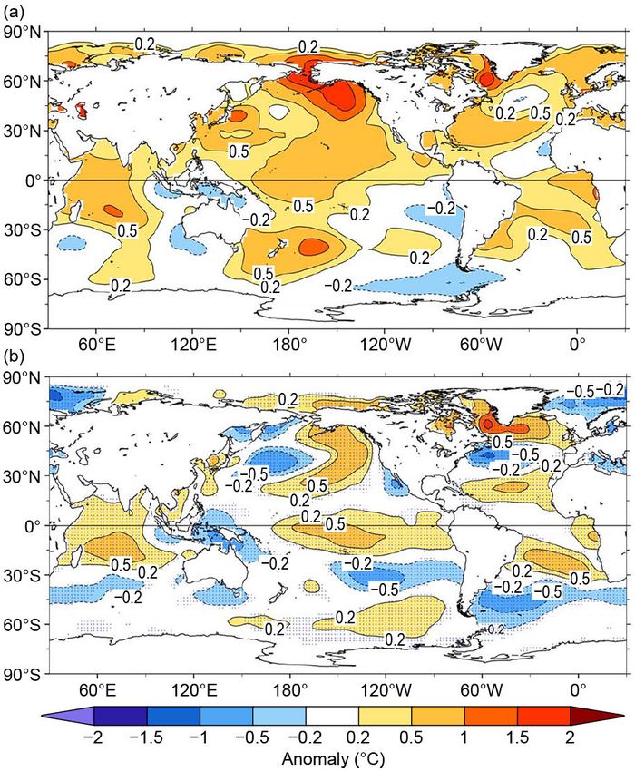
STATE OF THE CLIMATE IN 2019
                          Global Oceans

                                                                         Editors

                                                                     Jessica Blunden
                                                                      Derek S. Arndt

                                                                     Chapter Editors

                                                                                                                  Downloaded from http://journals.ametsoc.org/bams/article-pdf/101/8/S129/4991601/bamsd200105.pdf by guest on 14 October 2020
                                                                  Peter Bissolli
                                                              Howard J. Diamond
                                                          Matthew L. Druckenmiller
                                                               Robert J. H. Dunn
                                                               Catherine Ganter
                                                                Nadine Gobron
                                                                 Rick Lumpkin
                                                         Jacqueline A. Richter-Menge
                                                                     Tim Li
                                                              Ademe Mekonnen
                                                             Ahira Sánchez-Lugo
                                                                Ted A. Scambos
                                                               Carl J. Schreck III
                                                             Sharon Stammerjohn
                                                              Diane M. Stanitski
                                                                Kate M. Willett

                                                                     Technical Editor

                                                                     Andrea Andersen

                                                   BAMS Special Editor for Climate

                                                                      Richard Rosen

                                                  American Meteorological Society

AU G U S T 2 0 2 0 | S t a t e o f t h e C l i m a t e i n 2 0 1 9                      3. GLOBAL OCEANS   S130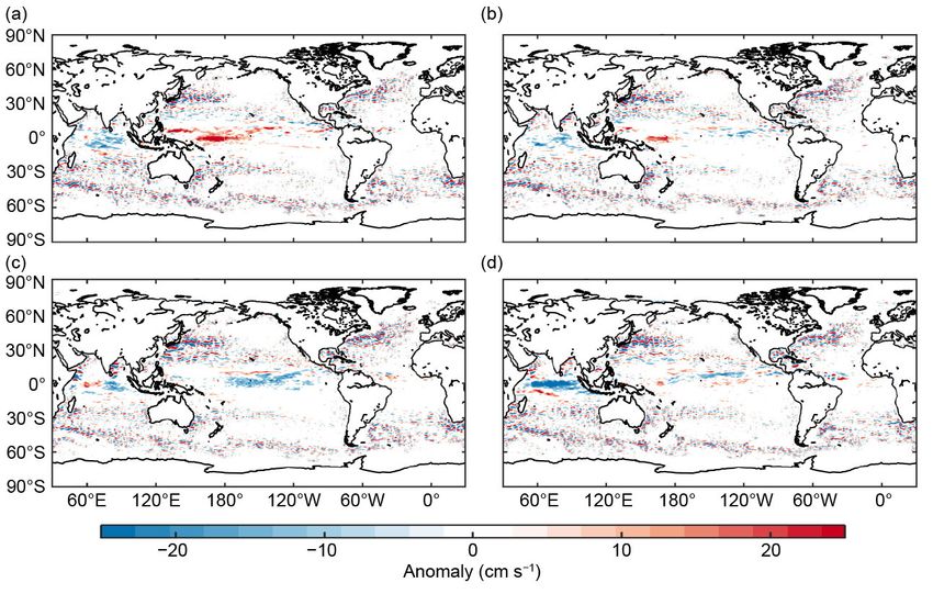
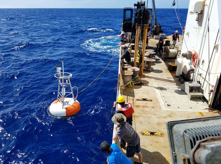
Cover credit:
2019 PIRATA Northeast Extension cruise on the NOAA ship Ronald H. Brown
Photo courtesy Dr. Renellys Perez (NOAA /AOML)

                                                                                                                Downloaded from http://journals.ametsoc.org/bams/article-pdf/101/8/S129/4991601/bamsd200105.pdf by guest on 14 October 2020
Global Oceans is one chapter from the State of the Climate in 2019 annual report and is avail-
able from https://doi.org/10.1175/BAMS-D-20-0105.1. Compiled by NOAA’s National Centers for
Environmental Information, State of the Climate in 2019 is based on contr1ibutions from scien-
tists from around the world. It provides a detailed update on global climate indicators, notable
weather events, and other data collected by environmental monitoring stations and instru-
ments located on land, water, ice, and in space. The full report is available from https://doi.org
/10.1175/2020BAMSStateoftheClimate.1.

How to cite this document:

Citing the complete report:
Blunden, J. and D. S. Arndt, Eds., 2020: State of the Climate in 2019. Bull. Amer. Meteor. Soc.,
101 (8), Si–S429, https://doi.org/10.1175/2020BAMSStateoftheClimate.1.

Citing this chapter:
Lumpkin, R. L., Ed., 2020: Global Oceans [in “State of the Climate in 2019"]. Bull. Amer. Meteor.
Soc., 101 (8), S129–S183, https://doi.org/10.1175/BAMS-D-20-0105.1.

Citing a section (example):
Franz, B. A., I. Cetinić, J. P. Scott, D. A. Siegel, and T. K. Westberry, 2020: Global ocean phyto-
plankton [in “State of the Climate in 2019"]. Bull. Amer. Meteor. Soc., 101 (8), S163–S169, https://
doi.org/10.1175/BAMS-D-20-0105.1.

  AU G U S T 2 0 2 0 | S t a t e o f t h e C l i m a t e i n 2 0 1 9                  3. GLOBAL OCEANS   S131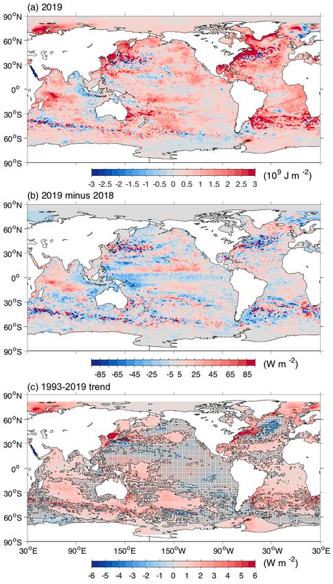
Editor and Author Affiliations (alphabetical by name)

Baringer, Molly, NOAA/OAR Atlantic Oceanographic and Meteorological                   Lankhorst, Matthias, Scripps Institution of Oceanography, University of
     Laboratory, Miami, Florida                                                            California at San Diego, La Jolla, California
Bif, Mariana B., Monterey Bay Aquarium Research Institute, Moss Landing,              Lee, Tong, NASA Jet Propulsion Laboratory, Pasadena, California
     California                                                                       Leuliette, Eric, NOAA/NESDIS Center for Satellite Applications and Research,
Boyer, Tim, NOAA/NESDIS National Centers for Environmental Information,                    College Park, Maryland
     Silver Spring, Maryland                                                          Li, Feili, College of Sciences, Georgia Institute of Technology, Atlanta, Georgia
Bushinsky, Seth M., University of Hawai'i at Mānoa, Honolulu, Hawai'i                 Lindstrom, Eric, Saildrone Inc., Alameda, California
Carter, Brendan R., Joint Institute for the Study of the Atmosphere and Ocean,        Locarnini, Ricardo, NOAA/NESDIS National Centers for Environmental
     University of Washington, and NOAA/OAR Pacific Marine Environmental                   Information, Silver Spring, Maryland
     Laboratory, Seattle, Washington                                                  Lozier, Susan, College of Sciences, Georgia Institute of Technology, Atlanta,
Cetinić, Ivona, NASA Goddard Space Flight Center, Greenbelt, Maryland, and                 Georgia
     Universities Space Research Association, Columbia, Maryland                      Lumpkin, Rick, NOAA/OAR Atlantic Oceanographic and Meteorological
Chambers, Don P., College of Marine Science, University of South Florida, St.              Laboratory, Miami, Florida
     Petersburg, Florida                                                              Lyman, John M., NOAA/OAR Pacific Marine Environmental Laboratory, Seattle,

                                                                                                                                                                           Downloaded from http://journals.ametsoc.org/bams/article-pdf/101/8/S129/4991601/bamsd200105.pdf by guest on 14 October 2020
Cheng, Lijing, International Center for Climate and Environment Sciences,                  Washington, and Joint Institute for Marine and Atmospheric Research,
     Institute of Atmospheric Physics, Chinese Academy of Sciences, Beijing,               University of Hawai'i, Honolulu, Hawai'i
     China                                                                            Marra, John J., NOAA/NESDIS National Centers for Environmental Information,
Chiba, Sanai, Japan Agency for Marine-Earth Science and Technology,                        Honolulu, Hawai'i
     Yokosuka, Japan                                                                  Meinen, Christopher S., NOAA/OAR Atlantic Oceanographic and
Dai, Minhan, Xiamen University, Xiamen, China                                              Meteorological Laboratory, Miami, Florida
Domingues, Catia M., Institute for Marine and Antarctic Studies, University of        Merrifield, Mark A., Scripps Institution of Oceanography, University of
     Tasmania, Antarctic Climate and Ecosystems Cooperative Research Centre,               California at San Diego, La Jolla, California
     and Australian Research Council’s Centre of Excellence for Climate System        Mitchum, Gary T., College of Marine Science, University of South Florida, St.
     Science, Hobart, Tasmania, Australia                                                  Petersburg, Florida
Dong, Shenfu, NOAA/OAR Atlantic Oceanographic and Meteorological                      Moat, Ben, National Oceanography Centre, Southampton, United Kingdom
     Laboratory, Miami, Florida                                                       Monselesan, Didier, CSIRO Oceans and Atmosphere, Hobart, Tasmania,
Fassbender, Andrea J., Monterey Bay Aquarium Research Institute, Moss                      Australia
     Landing, California                                                              Nerem, R. Steven, Colorado Center for Astrodynamics Research, Cooperative
Feely, Richard A., NOAA/OAR Pacific Marine Environmental Laboratory,                       Institute for Research in Environmental Sciences, University of Colorado
     Seattle, Washington                                                                   Boulder, Boulder, Colorado
Frajka-Williams, Eleanor, National Oceanography Centre, Southampton,                  Perez, Renellys C., NOAA/OAR Atlantic Oceanographic and Meteorological
     United Kingdom                                                                        Laboratory, Miami, Florida
Franz, Bryan A., NASA Goddard Space Flight Center, Greenbelt, Maryland                Purkey, Sarah G., Scripps Institution of Oceanography, University of California
Gilson, John, Scripps Institution of Oceanography, University of California at             at San Diego, La Jolla, California
     San Diego, La Jolla, California                                                  Rayner, Darren, National Oceanography Centre, Southampton, United Kingdom
Goni, Gustavo, NOAA/OAR Atlantic Oceanographic and Meteorological                     Reagan, James, Earth System Science Interdisciplinary Center/Cooperative
     Laboratory, Miami, Florida                                                            Institute for Satellite Earth System Studies, University of Maryland, College
Hamlington, Benjamin D., NASA Jet Propulsion Laboratory, Pasadena,                         Park, Maryland and NOAA/NESDIS National Centers for Environmental
     California                                                                            Information, Silver Spring, Maryland
Hu, Zeng-Zhen, NOAA/NCEP Climate Prediction Center, College Park, Maryland            Rome, Nicholas, Consortium for Ocean Leadership, Washington, D.C.
Huang, Boyin, NOAA/NESDIS National Centers for Environmental Information,             Sanchez-Franks, Alejandra, National Oceanography Centre, Southampton,
     Asheville, North Carolina                                                             United Kingdom
Ishii, Masayoshi, Department of Atmosphere, Ocean and Earth System                    Schmid, Claudia, NOAA/OAR Atlantic Oceanographic and Meteorological
     Modeling Research, Meteorological Research Institute, Japan                           Laboratory, Miami, Florida
     Meteorological Agency, Tsukuba, Japan                                            Scott, Joel P., NASA Goddard Space Flight Center, Greenbelt, Maryland and
Jevrejeva, Svetlana, National Oceanography Centre, Liverpool, United                       Science Application International Corporation, Beltsville, Maryland
     Kingdom                                                                          Send, Uwe, Scripps Institution of Oceanography, University of California at San
Johns, William E., Rosenstiel School of Marine and Atmospheric Science,                    Diego, La Jolla, California
     University of Miami, Miami, Florida                                              Siegel, David A., University of California at Santa Barbara, Santa Barbara,
Johnson, Gregory C., NOAA/OAR Pacific Marine Environmental Laboratory,                     California
     Seattle, Washington                                                              Smeed, David A., National Oceanography Centre, Southampton, United
Johnson, Kenneth S., Monterey Bay Aquarium Research Institute, Moss                        Kingdom
     Landing, California                                                              Speich, Sabrina, École Normale Supérieure Laboratoire de Météorologie
Kennedy, John, Met Office Hadley Centre, Exeter, United Kingdom                            Dynamique, Paris, France
Kersalé, Marion, Cooperative Institute for Marine and Atmospheric Studies,            Stackhouse Jr., Paul W., NASA Langley Research Center, Hampton, Virginia
     University of Miami, Miami, Florida and NOAA/OAR Atlantic Oceanographic          Sweet, William, NOAA/NOS Center for Operational Oceanographic Products
     and Meteorological Laboratory (AOML), Miami, Florida                                  and Services, Silver Spring, Maryland
Killick, Rachel E., Met Office Hadley Centre, Exeter, United Kingdom                  Takeshita, Yuichiro, Monterey Bay Aquarium Research Institute, Moss
Landschützer, Peter, Max Planck Institute for Meteorology, Hamburg, Germany                Landing, California

                 AU G U S T 2 0 2 0 | S t a t e o f t h e C l i m a t e i n 2 0 1 9                                                    3. GLOBAL OCEANS            S132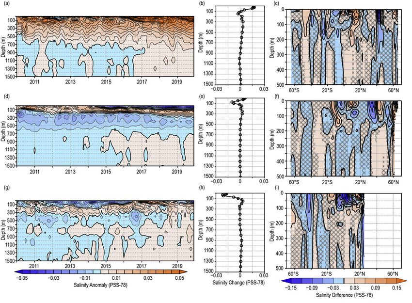
Thompson, Philip R., Department of Oceanography, University of Hawai'i at             Weller, Robert A., Woods Hole Oceanographic Institution, Woods Hole,
    Mānoa, Honolulu, Hawai'i                                                              Massachusetts
Triñanes, Joaquin A., Laboratory of Systems, Technological Research Institute,        Westberry, Toby K., Oregon State University, Corvallis, Oregon
    Universidad de Santiago de Compostela, Campus Universitario Sur,                  Widlansky, Matthew J., Joint Institute for Marine and Atmospheric Research,
    Santiago de Compostela, Spain; NOAA/OAR Atlantic Oceanographic and                    University of Hawai'i at Mānoa, Honolulu, Hawai'i
    Meteorological Laboratory, Miami, Florida, and Cooperative Institute for          Wijffels, Susan E., Woods Hole Oceanographic Institution, Woods Hole,
    Marine and Atmospheric Studies, University of Miami, Miami, Florida                   Massachusetts
Visbeck, Martin, GEOMAR Helmholtz Centre for Ocean Research Kiel, Kiel,               Wilber, Anne C., Science Systems and Applications, Inc., Hampton, Virginia
    Germany                                                                           Yu, Lisan, Woods Hole Oceanographic Institution, Woods Hole, Massachusetts
Volkov, Denis L., Cooperative Institute for Marine and Atmospheric Studies,           Yu, Weidong, National Marine Environmental Forecasting Center, State Oceanic
    University of Miami, Miami, Florida and NOAA/OAR Atlantic Oceanographic               Administration, Beijing, China
    and Meteorological Laboratory (AOML), Miami, Florida                              Zhang, Huai-Min, NOAA/NESDIS National Centers for Environmental
Wanninkhof, Rik, NOAA/OAR Atlantic Oceanographic and Meteorological                       Information, Asheville, North Carolina
    Laboratory, Miami, Florida

                                                                                                                                                                     Downloaded from http://journals.ametsoc.org/bams/article-pdf/101/8/S129/4991601/bamsd200105.pdf by guest on 14 October 2020
        Editorial and Production Team

Andersen, Andrea, Technical Editor, TeleSolv Consulting LLC, NOAA/NESDIS              Misch, Deborah J., Graphics Support, Innovative Consulting & Management
    National Centers for Environmental Information, Asheville, North Carolina             Services, LLC, NOAA/NESDIS National Centers for Environmental
Griffin, Jessicca, Graphics Support, Cooperative Institute for Satellite Earth            Information, Asheville, North Carolina
    System Studies, North Carolina State University, Asheville, North Carolina        Riddle, Deborah B., Graphics Support, NOAA/NESDIS National Centers for
Hammer, Gregory, Content Team Lead, Communications and Outreach, NOAA/                    Environmental Information, Asheville, North Carolina
    NESDIS National Centers for Environmental Information, Asheville, North           Veasey, Sara W., Visual Communications Team Lead, Communications and
    Carolina                                                                              Outreach, NOAA/NESDIS National Centers for Environmental Information,
Love-Brotak, S. Elizabeth, Lead Graphics Production, NOAA/NESDIS National                 Asheville, North Carolina
    Centers for Environmental Information, Asheville, North Carolina

                 AU G U S T 2 0 2 0 | S t a t e o f t h e C l i m a t e i n 2 0 1 9                                                3. GLOBAL OCEANS           S133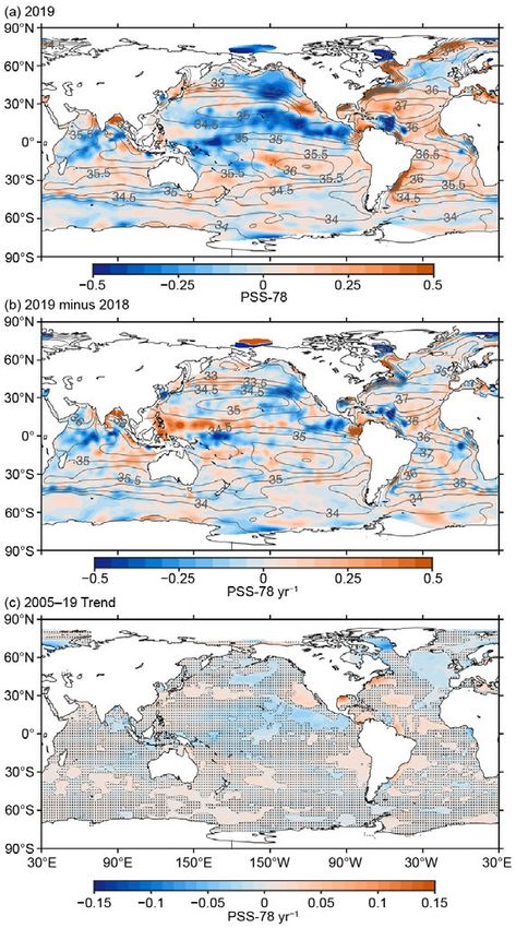
3. Table of Contents

List of authors and affiliations...................................................................................................S132
a. Overview ..................................................................................................................................S135
b. Sea surface temperature.........................................................................................................S136
c. Ocean heat content.................................................................................................................S140
d. Salinity......................................................................................................................................S144
		 1. Introduction.................................................................................................................S144
		 2. Sea surface salinity......................................................................................................S144
		 3. Subsurface salinity.......................................................................................................S146
e. Global ocean heat, freshwater, and momentum fluxes.......................................................S149

                                                                                                                                                               Downloaded from http://journals.ametsoc.org/bams/article-pdf/101/8/S129/4991601/bamsd200105.pdf by guest on 14 October 2020
		 1. Surface heat fluxes......................................................................................................S150
		 2. Surface freshwater fluxes............................................................................................S151
		 3. Wind stress...................................................................................................................S152
		 4. Long-term perspective................................................................................................S152
f. Sea level variability and change.............................................................................................S153
g. Suface currents........................................................................................................................S156
		 1. Pacific Ocean................................................................................................................S156
		 2. Indian Ocean................................................................................................................S158
		 3. Atlantic Ocean..............................................................................................................S158
h. Atlantic meridional overturning circulation and associated heat transport......................S159
i. Global ocean phytoplankton...................................................................................................S163
     Sidebar 3.1: BioGeoChemical Argo......................................................................................S167
j. Global ocean carbon cycle.......................................................................................................S170
		 1. Introduction.................................................................................................................S170
		 2. Air–sea carbon dioxide fluxes.....................................................................................S170
		 3. Large-scale carbon and pH changes in the ocean interior.......................................S173
     Sidebar 3.2: OceanObs’19.................................................................................................... S174
Appendix: Acronym List..............................................................................................................S176
References....................................................................................................................................S178

*Please refer to Chapter 8 (Relevant datasets and sources) for a list of all climate variables and
datasets used in this chapter for analyses, along with their websites for more information and
access to the data.

    AU G U S T 2 0 2 0 | S t a t e o f t h e C l i m a t e i n 2 0 1 9                                                             3. GLOBAL OCEANS     S134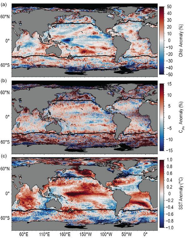
3. GLOBAL OCEANS
Rick Lumpkin, Ed.

a. Overview—R. Lumpkin
   In this chapter, we examine the state of the global oceans in 2019, focusing both on changes from
2018 to 2019 and on the longer-term perspective. Sidebars focus on the significant and ongoing
scientific results from the growing array of Argo floats measuring biogeochemical properties, and
on the OceanObs’19 conference, a once-per-decade event focusing on sustaining and enhancing

                                                                                                                  Downloaded from http://journals.ametsoc.org/bams/article-pdf/101/8/S129/4991601/bamsd200105.pdf by guest on 14 October 2020
the global ocean-observing system.
   The year 2019 marks the eighth consecutive year that global mean sea level increased relative to
the previous year, reaching a new record: 87.6 mm above the 1993 average (Fig. 3.14a) and peaking
in the middle of the year. The globally averaged 2019 sea surface temperature anomaly (SSTA)
was the second highest on record, surpassed only by the record El Niño year of 2016. The warm-
ing trend of ocean heat content (OHC) from 2004 to 2019 corresponds to a rate exceeding 0.20°C
decade-1 near the surface, declining to 30 W m−2 and were much larger than climatology in most of the central and eastern
tropical Indian Ocean basin (Fig. 3.10a). This heat gain was associated with increased surface
radiation (Fig. 3.10c) and drove increased turbulent heat loss to the atmosphere (Fig. 3.10d). In the
lead-up to the extreme dipole event, westward geostrophic current anomalies developed across
the basin, reaching maxima of ~40 cm s−1 at the peak of the dipole (Fig. 3.18). By the end of the
year, there was a significant east-to-west sea level anomaly gradient across the tropical Indian
Ocean (Fig. 3.15d).
   The tropical Pacific was characterized by a transition from a diminishing La Niña in 2018 to
the development of a weak El Niño by early 2019. Sustained negative values of the Oceanic Niño
Index over the last decade produced positive anomalies in the flux of CO2 from the ocean to the
atmosphere in the eastern tropical Pacific (Fig. 3.27c). In the North Pacific, sea surface temperatures
(SSTs) increased significantly in the latter half of 2019 (Figs. 3.2c,d), leading to the reemergence
of a “warm blob” that was associated with a decrease in precipitation (Fig. 3.11d) and winds (Fig.
3.12a). In the northwest subpolar Pacific and western Bering Sea, positive anomalies in the flux
of CO2 from the ocean to the atmosphere were related to sustained above-average SSTA there
(Fig. 3.27c).

  AU G U S T 2 0 2 0 | S t a t e o f t h e C l i m a t e i n 2 0 1 9                    3. GLOBAL OCEANS   S135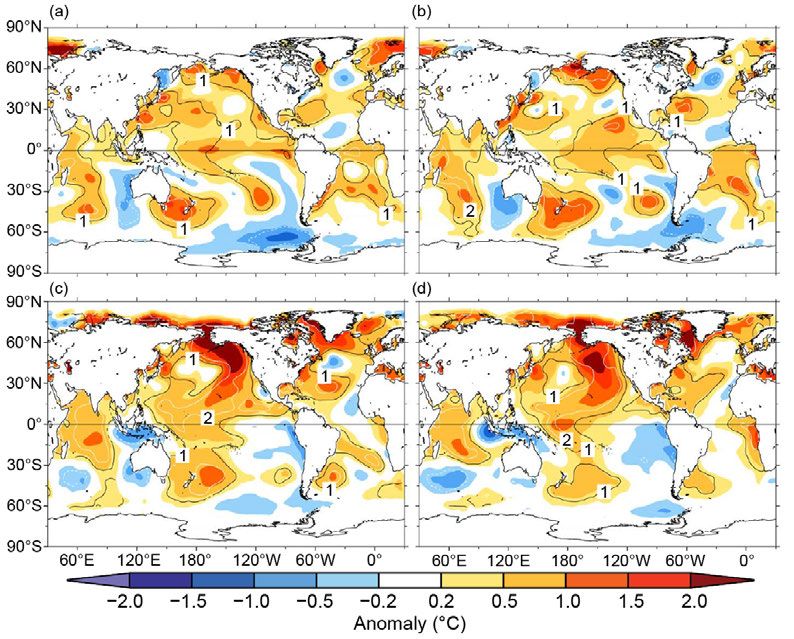
Positive SSTAs were observed in the tropical Atlantic, corresponding to the development of
an Atlantic Niño. The North Atlantic was characterized by a tripole-like SSTA pattern (Fig. 3.1a),
associated with positive net heat flux anomalies from 30°S to 60°N (Figs. 3.10a,b). Dramatic SST
increase in the Labrador Sea (Fig. 3.1a) was associated with the reduction of sea ice coverage.
Upper ocean heat content south of Greenland, which had been anomalously low since 2009,
increased in 2019 (Fig. 3.4a).
   The October 2018–September 2019 globally-averaged concentration of chlorophyll-a (chla)
varied from its 22-year monthly climatology by ±6% (Fig. 3.25b), while the concentration of phyto-
planktonic carbon (Cphy) varied by ±2% (Fig. 3.25d), indicating neutral El Niño–Southern Oscilla-
tion conditions. Regionally, chla was suppressed by 10%–30% where SST anomalies were positive,
while variations of Cphy were far less dramatic. This is because above-average SST anomalies are
associated with shallow mixed layers and thus increased light exposure to phytoplankton in that
layer, leading in turn to reduced cellular chla and a decoupling of chla and Cphy concentrations.
    For this year’s report, we are pleased to re-introduce a section focusing on the Atlantic me-

                                                                                                                Downloaded from http://journals.ametsoc.org/bams/article-pdf/101/8/S129/4991601/bamsd200105.pdf by guest on 14 October 2020
ridional overturning circulation (AMOC). In this section, we learn that decadal-scale variability
of the southward deep western boundary current in the subtropical North Atlantic is poorly
correlated with the relatively constant (at these time scales) northward-flowing Florida Current,
and that rapid changes in the Florida Current can be driven by hurricanes; the passage of Hur-
ricane Dorian coincided with the lowest transport measurement of the current ever recorded.
The strength of the AMOC in the subtropical North Atlantic significantly decreased between
2004–08 and 2008–12 (Smeed et al. 2018) and has remained lower since then (Moat et al. 2019,
2020), consistent with a reduction of deep water production farther north. Direct measurements
in the subpolar North Atlantic, collected by the Overturning in the Subpolar North Atlantic Pro-
gram (OSNAP) array, challenge the conventional wisdom that deep water formation changes are
strongly associated with changes in convection in the Labrador Sea, instead pointing to changes
solely in the Irminger and Iceland basins (Lozier et al. 2019b). In the South Atlantic, interannual
variations in the AMOC strength are associated with both density-driven and pressure-driven
fluctuations (Meinen et al. 2018).

b. Sea surface temperature —B. Huang, Z.-Z. Hu, J. J. Kennedy, and H.-M. Zhang
   The sea surface temperature (SST) over the global ocean (all water surfaces, including seas and
great lakes) in 2019 is assessed using three updated products of SST and its uncertainty. These
products are the Extended Reconstruction Sea-Surface Temperature version 5 (ERSSTv5; Huang
et al. 2017, 2020), Daily Optimum Interpolation SST version 2 (DOISST; Reynolds et al. 2007), and
U.K. Met Office Hadley Centre SST (HadSST.3.1.1.0 and HadSST.4.0.0.0; Kennedy et al. 2011a,b,
2019). See the State of the Climate in 2018 report for details of these calculations. SST anomalies
(SSTAs) are calculated relative to their own climatologies over 1981–2010. The magnitudes of
SSTAs are compared against SST standard deviations (std. dev.) over 1981–2010.
   Averaged over the global oceans, ERSSTv5 analysis shows that SSTAs increased significantly
from 0.33° ± 0.03°C in 2018 to 0.41° ± 0.03°C in 2019. The uncertainty in ERSSTv5 is slightly smaller
than that in ERSSTv4, as determined by a Student’s t-test using a 1000-member ensemble based
on ERSSTv5 with randomly drawn parameter values within reasonable ranges in the SST recon-
structions (Huang et al. 2015, 2020).
   Figure 3.1a shows annually averaged SSTA in 2019. In most of the North Pacific, SSTAs were
between +0.5°C and +1.0°C except for near the Bering Strait (+1.5°C), about +0.5°C in the west-
ern South Pacific, and between −0.2°C and +0.2°C in the eastern South Pacific. The extreme
warm event in the northeast Pacific is referred to as Blob 2.0 (Amaya et al. 2020). In the Atlantic,
SSTAs were between +0.2°C and +0.5°C except for the tropical North Atlantic and near the coast
of Africa (−0.2°C to 0°C), central North Atlantic near 45°N and 30°W (0°C), and the Labrador Sea
(about +1.5°C). In the Indian Ocean, SSTAs were +0.5°C west of 90°E and slightly below average

   AU G U S T 2 0 2 0 | S t a t e o f t h e C l i m a t e i n 2 0 1 9                 3. GLOBAL OCEANS   S136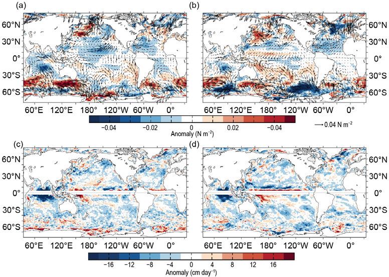
(−0.2°C) in the regions surrounding
                                                                               the Maritime Continent and western
                                                                               Australia.
                                                                                  In comparison with averaged SST
                                                                               in 2018, the averaged SST in 2019 in-
                                                                               creased by +1.0°C to +1.5°C south of
                                                                               Greenland (Fig. 3.1b) and was +0.2°C
                                                                               to +0.5°C higher in the northeastern
                                                                               Pacific stretching from Alaska and
                                                                               Canada toward the central North
                                                                               Pacific, in the central-eastern tropi-
                                                                               cal Pacific, in the Pacific sector of
                                                                               the Southern Ocean south of 50°S,
                                                                               in the tropical North Atlantic over

                                                                                                                                Downloaded from http://journals.ametsoc.org/bams/article-pdf/101/8/S129/4991601/bamsd200105.pdf by guest on 14 October 2020
                                                                               10°–30°N, in the tropical South At-
                                                                               lantic over 10°–30°S, in the eastern
                                                                               equatorial Atlantic, and in most of
                                                                               the Indian Ocean. In contrast, the
                                                                               SST decreased by −0.2°C to −0.5°C
                                                                               in the North Atlantic poleward of
                                                                               60°N, in the subtropical North At-
                                                                               lantic between 30°N and 45°N, in
                                                                               the subpolar South Atlantic south
                                                                               of 35°S, in the northwestern North
                                                                               Pacific between 30°N and 65°N, in
                                                                               the western tropical Pacific, in the
Fig. 3.1. (a) Annually averaged SSTAs (°C) in 2019 and (b) difference of       subtropical South Pacific between
annually averaged SSTAs between 2019 and 2018. SSTAs are relative              20°S and 40°S, and in the southern
to 1981–2010 climatology. The SST difference in (b) is significant at          Indian Ocean between 30°S and
95% level in stippled areas.                                                   45°S. These SST changes are statis-
                                                                               tically significant at the 95% confi-
                                                                               dence level based on an ensemble
                                                                               analysis of 1000 members.
               The pattern of cooling in the western North Pacific and warming in the eastern North Pacific
            (Fig. 3.1b) may be associated with a shift of the Pacific Decadal Oscillation (PDO; Mantua and Hare
            2002) index from a negative phase in 2018 to near neutral in 2019. The warming in the central-
            eastern tropical Pacific (Fig. 3.1b) is associated with a transition from the weak La Niña over 2017/18
            to the weak El Niño over 2018/19. The warming in the western Indian Ocean is associated with an
            enhanced Indian Ocean dipole (IOD; Saji et al. 1999; see section 4h) from 0.3°C in 2018 to 0.8°C
            in 2019. The monthly IOD index reached its highest level since 1997 in October 2019 that affected
            patterns of precipitation and precipitation-minus-evaporation over the Maritime Continent and
            Australia (Fig. 3.11, see section 7h4).
               The seasonal variations in SST in 2019 were profound. In most of the North Pacific, SSTAs were
            +0.2°C to +0.5°C (1 std. dev. above average) in December–February (DJF) and March–May (MAM)
            (Figs. 3.2a,b). The anomaly increase ranged from +0.5°C to +2.0°C (2 std. dev.) in June–August (JJA)
            and September–November (SON; Figs. 3.2c,d). In contrast, in the western South Pacific, SSTAs
            were high (+1.0°C; ≥2 std. dev.) in DJF, MAM, and JJA and lower in SON, albeit still above average
            (+0.5°C; ≥1 std. dev.). In the eastern South Pacific, SSTAs persisted at about −0.2°C, although
            these anomalies stretched farther westward and equatorward in JJA and SON (Figs. 3.2c,d) than
            in DJF and MAM (Figs. 3.2a,b) following the evolution of the equatorial Pacific cold tongue. In the

             AU G U S T 2 0 2 0 | S t a t e o f t h e C l i m a t e i n 2 0 1 9                       3. GLOBAL OCEANS   S137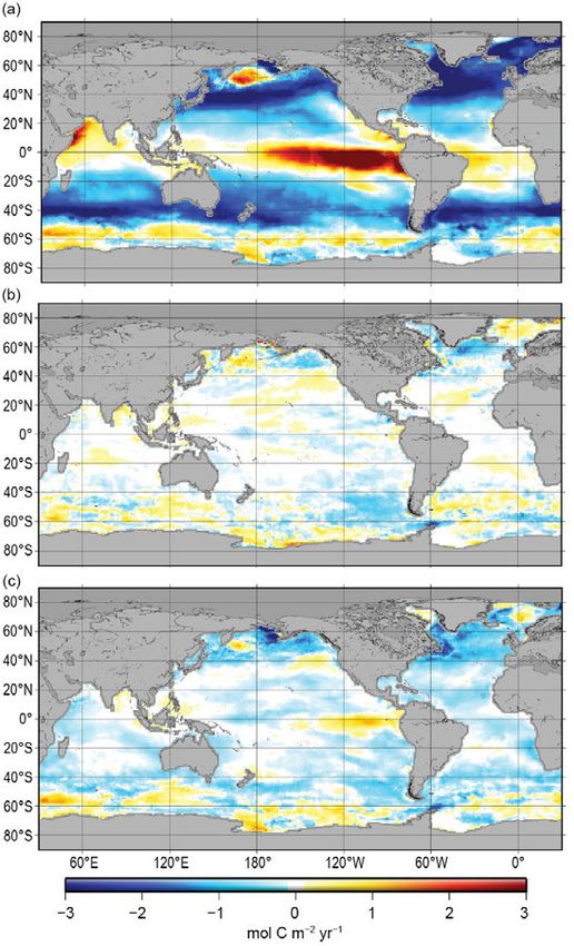
Southern Ocean between the date line and 30°W, SSTAs were −0.5°C to −1.5°C (1 std. dev. below
          average) in DJF and MAM but were closer to average in JJA and SON.
             It should be noted that there was an unusual heat content anomaly during the summer and
          spring around New Zealand (Figs. 3.2a,b). The Tasman Sea has seen a series of marine heatwaves
          in the past few years (Oliver et al. 2017; Perkins-Kirkpatrick et al. 2019; Babcock et al. 2019). In
          December 2019, SSTAs to the east of New Zealand were significantly above average.
             In the western Indian Ocean, SSTAs persisted in the range of +0.5°C to +1.0°C (1–2 std.
          dev. above average) throughout all seasons (Fig. 3.2), while SSTAs were from −0.5°C to −1.0°C
          (1–2 std. dev. below average) in the eastern Indian Ocean and regions of the Maritime Continent.
          The warm western Indian Ocean and the cold southeastern Indian Ocean resulted in an extremely
          strong positive phase of the IOD event and the highest IOD index value since 1997.
             Along the coasts of the Arctic, SSTs were near average in DJF and MAM (Figs. 3.2a,b) but above
          average (+1.0°C to +2.0°C; ≥2 std. dev.) in JJA and SON (Figs. 3.2c,d), which may be directly associ-
          ated with the reduction of sea ice concentration. Similarly, south of Greenland, SSTs were near

                                                                                                                            Downloaded from http://journals.ametsoc.org/bams/article-pdf/101/8/S129/4991601/bamsd200105.pdf by guest on 14 October 2020
          average in DJF and MAM but significantly above average in JJA and SON (+1.0°C to +2.0°C; ≥2 std.
          dev.), associated with the reduction of sea ice concentration in these areas. In the Labrador Sea,
          SSTAs were high in JJA and SON but lower in DJF and MAM.
             In the northern North Atlantic between 60°N and 80°N, above-average SSTs persisted through-
          out all seasons (+0.5°C to 1.0°C; 1 to 2 std. dev.). In the North Atlantic between 30°N and 60°N,
          SSTAs were negative (–0.5°C) in DJF, MAM, and JJA (Figs. 3.2a,b,c) but closer to average in SON
          (Fig. 3.2d). In the tropical North Atlantic, SSTAs were slightly below average (−0.5°C) throughout
          all seasons. In the equatorial Atlantic, SSTAs were +0.5°C above average in DJF and MAM, weak-
          ening in JJA, and strengthening again in SON, associated with the emergence of a weak Atlantic
          Niño that usually peaks in JJA (Chang et al. 2006). In the subtropical South Atlantic, SSTAs were

Fig. 3.2. Seasonally averaged SSTAs of ERSSTv5 (°C; shading) for (a) Dec–Feb 2018/19, (b) Mar–May 2019, (c) Jun–Aug 2019,
and (d) Sep–Nov 2019. The normalized seasonal mean SSTA based on seasonal mean 1 std. dev. over 1981–2010, indicated
by contours of −1 (dashed white), 1 (solid black), and 2 (solid white).

            AU G U S T 2 0 2 0 | S t a t e o f t h e C l i m a t e i n 2 0 1 9                  3. GLOBAL OCEANS    S138
+0.5°C to +1.0°C (1 to 2 std. dev.) in DJF and MAM, and the area of warm SSTAs was reduced in
JJA and further diminished in SON.
Overall, the global ocean warming trends of SSTs since the 1950s remained significant (Figs.
3.3a,b; Table 3.1), with noticeably higher SSTAs in 2019 (+0.41°C) than in 2018 (+0.33°C). The
year 2019 was the second-warmest year since 1950 after the record year of 2016 (+0.44°C). The
linear trends of globally annually averaged SSTAs were 0.10° ± 0.01°C decade−1 over 1950–2019
(Table 3.1). The warming appeared largest in the tropical Indian Ocean (Fig. 3.3e; 0.14° ± 0.02°C
decade−1) and smallest in the North Pacific (Fig. 3.3d; 0.09° ± 0.03°C decade−1). The uncertainty of
the trends represents the 95% confidence level of the linear fitting uncertainty and 1000-member
data uncertainty.
Table 3.1. Linear trends (°C decade –1) of annually and regionally averaged SSTAs from ERSSTv5, HadSST3,
and DOISST. The uncertainties at 95% confidence level are estimated by accounting for the effective
sampling number quantified by lag-1 auto correlation on the degrees of freedom of annually-averaged
Downloaded from http://journals.ametsoc.org/bams/article-pdf/101/8/S129/4991601/bamsd200105.pdf by guest on 14 October 2020
SST series.
Product Region 2000–2019 (°C decade –1) 1950–2019 (°C decade –1)
HadSST.3.1.1.0 Global 0.140 ± 0.065 0.086 ± 0.016
DOISST Global 0.156 ± 0.058 N/A
ERSSTv5 Global 0.170 ± 0.075 0.101 ± 0.013
ERSSTv5 Tropical Pacific (30°N–30°S) 0.188 ± 0.185 0.102 ± 0.028
ERSSTv5 North Pacific (30°–60°N) 0.287 ± 0.172 0.087 ± 0.028
ERSSTv5 Tropical Indian Ocean (30°N–30°S) 0.199 ± 0.098 0.141 ± 0.018
ERSSTv5 North Atlantic (30°–60°N) 0.142 ± 0.087 0.101 ± 0.034
ERSSTv5 Tropical Atlantic (30°N–30°S) 0.133 ± 0.097 0.109 ± 0.020
ERSSTv5 Southern Ocean (30°–60°S) 0.129 ± 0.060 0.099 ± 0.016
In addition to the long-term SST trend and interannual variability, interdecadal variations of
SSTAs can be seen in all ocean basins, although the amplitude of the variations was smaller in the
Southern Ocean (Fig. 3.3h). The variations associated with the Atlantic Multidecadal Variability
(Schlesinger and Ramankutty 1994) can be identified in the North Atlantic with warm periods in
the 1950s and over the 1990s–2010s, and a cold period over the 1960s–80s (Fig. 3.3f). Similarly,
SSTAs in the North Pacific (Fig. 3.3d) decreased from the 1950s to the late 1980s, followed by an
increase from the later 1980s to the 2010s.
SSTAs in ERSSTv5 were compared with those in DOISST, HadSST3.1.1.0, and HadSST.4.0.0.0. All
data sets were averaged to an annual 2° × 2° grid for comparison purposes. Comparisons (Fig. 3.3)
indicate that the SSTA departures of DOISST and HadSST.3.1.1.0 from ERSSTv5 are largely within
2 std. dev. (gray shading in Fig. 3.3). The 2 std. dev. was derived from a 1000-member ensemble
analysis based on ERSSTv5 (Huang et al. 2020) and centered to SSTAs of ERSSTv5. Overall, the
HadSST4.0.0.0 is more consistent with ERSSTv5 than HadSST.3.1.1.0. In the 2000s–10s, SSTAs in
the Southern Ocean were slightly higher in DOISST than in ERSSTv5. Previous studies (Huang
et al. 2015; Kent et al. 2017) have indicated that these SSTA differences are mostly attributed to
the differences in bias corrections to ship observations in those products. These SST differences
resulted in a slightly weaker SSTA trend in HadSST.3.1.1.0 over both 1950–2019 and 2000–19 (Table
3.1). In contrast, SST trends were slightly higher in DOISST over 2000–19.
AU G U S T 2 0 2 0 | S t a t e o f t h e C l i m a t e i n 2 0 1 9 3. GLOBAL OCEANS S139Downloaded from http://journals.ametsoc.org/bams/article-pdf/101/8/S129/4991601/bamsd200105.pdf by guest on 14 October 2020
Fig. 3.3. Annually averaged SSTAs (°C) of ERSSTv5 (solid white) and 2 std. dev. (gray shading) of ERSSTv5, SSTAs of DOISST
(solid green), and SSTAs of HadSST.3.1.1.0 (solid red) and HadSST.4.0.0.0 (dotted blue) in 1950–2019 except for (b). (a)
Global, (b) global in 1880–2019, (c) tropical Pacific Ocean, (d) North Pacific Ocean, (e) tropical Indian Ocean, (f) North At-
lantic Ocean, (g) tropical Atlantic Ocean, and (h) Southern Ocean. The year 2000 is indicated by a vertical black dotted line.
c. Ocean heat content—G. C. Johnson, J. M. Lyman, T. Boyer, L. Cheng, C. M. Domingues, J. Gilson, M. Ishii, R. E. Killick,
D. Monselesan, S. G. Purkey, and S. E. Wijffels
One degree of warming in the global ocean stores more than 1000 times the heat energy of one
degree of warming in the atmosphere owing to the higher mass of the ocean (280 times that of
the atmosphere) and the larger heat capacity of water (four times that of air). Ocean warming ac-
counts for about 89% of the total increase in Earth’s energy storage from 1960 to 2018, compared
to the atmosphere’s 1%. Ocean currents also transport substantial amounts of heat (Talley 2003).
Ocean heat storage and transport play large roles in the El Niño–Southern Oscillation (ENSO;
Johnson and Birnbaum 2017), tropical cyclone activity (Goni et al. 2009), sea level variability and
rates of change (section 3f), and melting of ice sheet outlet glaciers around Greenland (Castro de
la Guardia et al. 2015) and Antarctica (Schmidtko et al. 2014).
Maps of annual (Fig. 3.4) upper (0–700 m) ocean heat content anomaly (OHCA) relative to a
1993–2019 baseline mean are generated from a combination of in situ ocean temperature data
and satellite altimetry data following Willis et al. (2004), but using Argo (Riser et al. 2016) data
downloaded in January 2020. Near-global average seasonal temperature anomalies (Fig. 3.5) ver-
sus pressure from Argo data (Roemmich and Gilson 2009, updated) since 2004 and in situ global
AU G U S T 2 0 2 0 | S t a t e o f t h e C l i m a t e i n 2 0 1 9 3. GLOBAL OCEANS S140Downloaded from http://journals.ametsoc.org/bams/article-pdf/101/8/S129/4991601/bamsd200105.pdf by guest on 14 October 2020
Fig. 3.5. (a) Near-global (80°N–65°S, excluding continental
shelves, the Indonesian seas, and the Sea of Okhostk) inte-
grals of monthly ocean temperature anomalies (°C; updated
from Roemmich and Gilson 2009) relative to record-length
average monthly values, smoothed with a 5-month Hanning
filter and contoured at odd 0.02°C intervals (see color bar)
versus pressure and time. (b) Linear trend of temperature
anomalies over time for the length of the record in (a) plotted
versus pressure in °C decade−1 (orange line), and trend with
a Niño3.4 regression removed (blue line) following Johnson
and Birnbaum (2017).
estimates of OHCA (Fig. 3.6) for three pressure
Fig. 3.4. (a) Combined satellite altimeter and in situ ocean layers (0–700 m, 700–2000 m, and 2000–6000 m)
temperature data estimate of upper (0–700 m) OHCA from seven different research groups are also
(× 109 J m−2) for 2019 analyzed following Willis et al. (2004),
discussed.
but using an Argo monthly climatology and displayed
The 2018/19 tendency of 0–700 m OHCA
relative to the 1993–2019 baseline. (b) 2019 minus 2018
combined estimates of OHCA expressed as a local surface (Fig. 3.4b) in the Pacific shows a decrease along
heat flux equivalent (W m−2). For (a) and (b) comparisons, the equator, with a near-zonal band of increase
note that 95 W m−2 applied over one year results in a 3 × just to the north, consistent with the discharge
10 9 J m−2 change of OHCA. (c) Linear trend from 1993–2019 of heat from the equatorial region after the weak
of the combined estimates of upper (0–700 m) annual El Niño of 2018/19 and a decrease in eastward
OHCA (W m−2). Areas with statistically insignificant trends
surface current anomalies north of the equator
are stippled.
from 2018 to 2019 (see Fig. 3.17b). Outside of the
equatorial region in the Pacific, there are nearly
zonal bands of increases and decreases that tend to tilt equatorward to the west. Structures like
these are quite common in the OHCA tendency maps from previous years and are reminiscent
of Rossby wave dynamics. There are also, as usual, small-scale increases and decreases at eddy
scales especially visible in and poleward of the subtropical gyres. Throughout much of the Pacific,
the 2019 upper OHCA is generally above the long-term average (Fig. 3.4a), with the most notable
departures being patches of below-average values southwest and south of Hawaii and low values
in the Southern Ocean from Drake Passage to about 150°W.
AU G U S T 2 0 2 0 | S t a t e o f t h e C l i m a t e i n 2 0 1 9 3. GLOBAL OCEANS S141Fig. 3.6. (a) Annual average global integrals of in situ estimates of
upper (0–700 m) OHCA (ZJ; 1 ZJ = 1021 J) for 1993–2019 with standard
errors of the mean. The MRI/JMA estimate is an update of Ishii et al.
(2017). The CSIRO/ACE CRC / IMAS-UTAS estimate is an update of
Domingues et al. (2008). The PMEL /JPL /JIMAR estimate is an update
and refinement of Lyman and Johnson (2014). The NCEI estimate
follows Levitus et al. (2012). The Met Office Hadley Centre estimate
is computed from gridded monthly temperature anomalies (relative
to 1950–2019) following Palmer et al. (2007). The IAP/CAS estimate
is reported in Cheng et al. (2020). See Johnson et al. (2014) for de-
tails on uncertainties, methods, and datasets. For comparison, all
estimates have been individually offset (vertically on the plot), first
to their individual 2005–19 means (the best-sampled time period),
and then to their collective 1993 mean. (b) Annual average global
integrals of in situ estimates of intermediate (700–2000 m) OHCA for
1993–2018 with standard errors of the mean, and a long-term trend
Downloaded from http://journals.ametsoc.org/bams/article-pdf/101/8/S129/4991601/bamsd200105.pdf by guest on 14 October 2020
with one standard error uncertainty shown from 1992.4–2011.5 for
deep and abyssal (z > 2000 m) OHCA following Purkey and Johnson
(2010) but updated using all repeat hydrographic section data avail-
able from https://cchdo.ucsd.edu/ as of January 2020.
In the Indian Ocean, the 2018/19 tendency of 0–700-m OHCA (Fig. 3.4b) shows the strongest
increases in a near-zonal band that again tilts equatorward to the west, starting at about 12°S
well off the west coast of Australia and ending at about 6°S near Africa. The largest decreases are
observed in the eastern portion of the basin, just to the west of Indonesia and Australia, as well as
patchy decreases between 35°S and 20°S across the basin and south of Australia. Smaller increases
are evident across much of the Arabian Sea and the western portion of the Bay of Bengal. Upper
OHCA values for 2019 were above the 1993–2019 mean in much of the Indian Ocean (Fig. 3.4a),
with especially high values northeast of Madagascar and below-average values mostly found
west of Indonesia and Australia. This pattern is consistent with a positive Indian Ocean dipole
(IOD) pattern of SSTs (section 3b), which has been linked to bushfires in Australia and flooding
in East Africa (see sections 7h4 and 7e3, respectively). It is also consistent with the increase in
westward surface current anomalies along and south of the equator in the Indian Ocean from
2018 to 2019 (see Fig. 3.17b).
The 2018/19 tendencies of 0–700-m OHCA (Fig. 3.4b) in the Atlantic Ocean are generally toward
warming in the tropics and subtropics, as well as in the subpolar North Atlantic from northern
Europe to northern Canada. Large-scale 2018/19 cooling tendencies are located east of Argentina
and east of Canada from Nova Scotia to St. John’s, Newfoundland. The only large-scale regions
in the Atlantic with below-average heat content in 2019 (Fig. 3.4a) were east of Argentina and
north of Norway. In a change from recent years, upper OHCA in 2019 was above the 1993–2019
average south of Greenland, in the vicinity of the Irminger Sea, where a cold area had persisted
since around 2009 (see previous State of the Climate reports). However, the warm conditions off
the east coast of North America that have also persisted since around 2009 intensified further.
In 2019, there were no large areas in the North Atlantic that were cooler than average.
The large-scale statistically significant (Fig. 3.4c) regional patterns in the 1993–2019 local
linear trends of upper OHCA are quite similar to those from 1993–2018 (Johnson et al. 2019). The
limited areas with statistically significant negative trends are found mostly south of Greenland
in the North Atlantic, south of the Kuroshio Extension across the North Pacific, in portions of the
eastern South Pacific, and in the Red Sea. The much larger areas with statistically significant
positive trends include much of the rest of the Atlantic Ocean, the western tropical Pacific, the
central North Pacific, most of the Indian Ocean, most of the marginal seas except the Red Sea, and
AU G U S T 2 0 2 0 | S t a t e o f t h e C l i m a t e i n 2 0 1 9 3. GLOBAL OCEANS S142much of the South Pacific Ocean. The Arctic and portions of the Southern Ocean show warming
as well, although those regions have limited in situ data.
Near-global average seasonal temperature anomalies (Fig. 3.5a) from the start of 2004 through
the end of 2019 exhibit a clear record-length warming trend (Fig. 3.5b, orange line). In addition,
during El Niño events (e.g., 2009/10 and 2014–16) the surface-to-100-dbar is warmer than surround-
ing years and 100–400 dbar is cooler as the east-west tilt of the equatorial Pacific thermocline
flattens out (e.g., Roemmich and Gilson 2011; Johnson and Birnbaum 2017). The opposite pattern
holds during La Niña events (e.g., 2007/08 and 2010–12) as the equatorial Pacific thermocline
shoals in the east and deepens in the west. The overall warming trend (Fig. 3.5b, orange line)
from 2004 to 2019 exceeds 0.2°C decade−1 near the surface, declining to less than 0.03°C decade−1
below 300 dbar and about 0.01°C decade−1 by 2000 dbar. Removing a linear regression against the
Niño3.4 index, which is correlated with ocean warming rates (e.g., Johnson and Birnbaum 2017),
results in a decadal warming trend (Fig. 3.5b, blue line) that is slightly smaller in the upper 100
dbar, at about 0.18°C decade−1 near the surface and slightly larger than the simple linear trend
Downloaded from http://journals.ametsoc.org/bams/article-pdf/101/8/S129/4991601/bamsd200105.pdf by guest on 14 October 2020
from about 100 dbar to 300 dbar, as expected given the large El Niño near the end of the record.
Since the start of 2017, temperatures from the surface to almost 2000 dbar are higher than the
2004–19 average (Fig. 3.5a). While 2018 was slightly warmer than 2019 from 110–225 dbar, 2019
was as warm or warmer than all other years over the full measured depth range.
The analysis is extended back in time from the Argo period to 1993 using sparser, more hetero-
geneous historical data collected mostly from ships (e.g., Abraham et al. 2013). The six different
estimates of annual globally integrated 0–700-m OHCA (Fig. 3.6a) all reveal a large increase since
1993, with all of the analyses reporting 2019 as a record high. The globally integrated 700–2000-m
OCHA annual values (Fig. 3.6b) vary more among analyses, but all report 2019 as a record high,
and the long-term warming trend in this layer is also clear. Globally integrated OHCA values in
both layers vary more both from year to year for individual years and from estimate to estimate
in any given year prior to the achievement of a near-global Argo array around 2005. The water
column from 0–700 and 700–2000 m gained 14 (±5) and 6 (±1) Zettajoules (ZJ), respectively (means
and standard deviations given) from 2018 to 2019. Causes of differences among estimates are
discussed in G. C. Johnson et al. (2015).
The rate of heat gain from linear fits to each of the six global integral estimates of 0–700 m
OHCA from 1993 through 2019 (Fig. 3.6a) ranges from 0.36 (±0.06) to 0.41 (±0.04) W m−2 applied over
the surface area of Earth (Table 3.2).
Linear trends from 700 m to 2000 m Table 3.2. Trends of ocean heat content increase (in W m –2 applied over
over the same time period range from the 5.1 × 10¹⁴ m2 surface area of Earth) from seven different research
groups over three depth ranges (see Fig. 3.6 for details). For the 0–700
0.14 (±0.04) to 0.32 (±0.03) W m−2. m and 700–2000 m depth ranges, estimates cover 1993–2019, with
Trends in the 0–700-m layer all agree 5%–95% uncertainties based on the residuals taking their temporal
within their 5%–95% uncertainties, correlation into account when estimating degrees of freedom (Von
Storch and Zwiers 1999). The 2000–6000-m depth range estimate, an
but as noted in previous reports, update of Purkey and Johnson (2010), uses data from 1981 to 2019, but
the Pacific Marine Environmental the globally averaged first and last years are 1992.4 and 2011.5, again
Laboratory/Joint Institute of Marine with 5%–95% uncertainty.
and Atmsopheric Research/Jet Pro- Global ocean heat content trends (W m −2)
for three depth ranges
pulsion Laboratory (PMEL/JIMAR/
Research Group 0–700 m 700–2000 m 2000–6000 m
JPL) trend in the 700–2000 m layer,
MRI/JMA 0.36 ± 0.06 0.24 ± 0.05 —
which is quite sparsely sampled prior
to the start of the Argo era (circa CSIRO/ACE/CRC/IMAS/UTAS 0.40 ± 0.06 — —
2005), does not. Different methods PMEL/JPL/JIMAR 0.39 ± 0.13 0.32 ± 0.03 —
for dealing with under-sampled re- NCEI 0.39 ± 0.06 0.19 ± 0.06 —
gions in analyses likely cause this Met Office Hadley Centre 0.37 ± 0.13 0.14 ± 0.04 —
disagreement. For 2000–6000 m, IAP/CAS 0.41 ± 0.04 0.19 ± 0.01 —
the linear trend is 0.06 (±0.03) W m −2 Purkey and Johnson — 0.06 ± 0.03
AU G U S T 2 0 2 0 | S t a t e o f t h e C l i m a t e i n 2 0 1 9 3. GLOBAL OCEANS S143from June 1992 to July 2011, using repeat hydrographic section data collected from 1981 to 2019 to
update the estimate of Purkey and Johnson (2010). Summing the three layers (with their slightly
different time periods), the full-depth ocean heat gain rate for the period from approximately
1993 to 2019 ranges from 0.55 to 0.79 W m−2. Estimates starting circa 2005 have much smaller
uncertainties (e.g., Johnson et al. 2016).
d. Salinity—G. C. Johnson, J. Reagan, J. M. Lyman, T. Boyer, C. Schmid, and R. Locarnini
1) Introduction—G. C. Johnson and J. Reagan
Salinity, the fraction of dissolved salts in water, and temperature determine the density of
seawater at a given pressure. At high latitudes where vertical temperature gradients are small,
low near-surface salinity values can be responsible for much of the density stratification. At lower
latitudes, fresh near-surface barrier layers can limit the vertical extent of ocean exchange with
the atmosphere (e.g., Lukas and Lindstrom 1991). Salinity variability can alter the density pat-
terns that are integral to the global thermohaline circulation (e.g., Gordon 1986; Broecker 1991).
Downloaded from http://journals.ametsoc.org/bams/article-pdf/101/8/S129/4991601/bamsd200105.pdf by guest on 14 October 2020
One prominent limb of that circulation, the Atlantic meridional overturning circulation (AMOC;
section 3h), is particularly susceptible to changes in salinity (e.g., Liu et al. 2017). Salinity is a
largely conservative water property, indicating where a water mass was originally formed at
the surface and subducted into the ocean’s interior (e.g., Skliris et al. 2014). Where precipitation
dominates evaporation, near-surface conditions are fresher (i.e., along the Intertropical Conver-
gence Zone [ITCZ] and at high latitudes), and where evaporation dominates precipitation, they
are saltier (i.e., in the subtropics). With ~80% of the global hydrological cycle taking place over
the ocean (e.g., Durack 2015), near-surface salinity changes over time can serve as a broad-scale
rain gauge (e.g., Terray et al. 2012) used to diagnose hydrological cycle amplifications associated
with global warming (e.g., Durack et al. 2012). Finally, besides atmospheric freshwater fluxes,
other factors modify salinity, such as advection, mixing, entrainment, sea ice melt/freeze, and
river runoff (e.g., Ren et al. 2011).
To investigate interannual changes of subsurface salinity, all available salinity profile data are
quality controlled following Boyer et al. (2018) and then used to derive 1° monthly mean gridded
salinity anomalies relative to a long-term monthly mean for the period 1955–2012 (World Ocean
Atlas 2013 version 2 [WOA13v2]; Zweng et al. 2013) at standard depths from the surface to 2000-m
depth (Boyer et al. 2013). In recent years, the largest source of salinity profiles is the profiling
floats of the Argo program (Riser et al. 2016). These data are a mix of real-time (preliminary) and
delayed-mode (scientific quality controlled) observations. Hence, the estimates presented here
could change after all data are subjected to scientific quality control. The sea surface salinity (SSS)
analysis relies on Argo data downloaded in January 2020, with annual maps generated following
Johnson and Lyman (2012) as well as monthly maps of bulk (as opposed to skin) SSS data from
the Blended Analysis of Surface Salinity (BASS; Xie et al. 2014). BASS blends in situ SSS data with
data from the Aquarius (Le Vine et al. 2014; mission ended in June 2015), Soil Moisture and Ocean
Salinity (SMOS; Font et al. 2013), and recently from Soil Moisture Active Passive (SMAP; Fore et al.
2016) satellite missions. Despite the larger uncertainties of satellite data relative to Argo data,
their higher spatial and temporal sampling allows higher spatial and temporal resolution maps
than are possible using in situ data alone at present. All salinity values used in this section are
dimensionless and reported on the Practical Salinity Scale-78 (PSS-78; Fofonoff and Lewis 1979).
2) Sea surface salinity—G. C. Johnson and J. M. Lyman
Unlike sea surface temperature (SST), for which anomalies tend to be damped by air–sea heat
exchanges, SSS has no direct feedback with the atmosphere, so large-scale SSS anomalies can
more easily persist over years. For instance, the 2019 fresh subpolar SSS anomaly observed in
the northeast Pacific (Fig. 3.7a) arguably began in 2016, centered more in the central subpolar
North Pacific, shifting eastward and building somewhat in strength and size between then and
AU G U S T 2 0 2 0 | S t a t e o f t h e C l i m a t e i n 2 0 1 9 3. GLOBAL OCEANS S144now (see previous State of the Climate re-
ports). This fresh anomaly may be associated
with the marine heat waves in the area that
occurred in 2014–16 (e.g., Gentemann et al.
2017) and again in 2019 (see Fig. 3.1a). A fresh
anomaly like this one would tend to increase
stratification and reduce the ability of storms
to deepen the mixed layer into colder sub-
surface water during winter, possibly even
promoting warm SST anomalies.
In the tropical Pacific, the fresh 2019 SSS
anomaly (Fig. 3.7a) observed over much of
the ITCZ and South Pacific Convergence Zone
(SPCZ) began around 2015 (see previous State
Downloaded from http://journals.ametsoc.org/bams/article-pdf/101/8/S129/4991601/bamsd200105.pdf by guest on 14 October 2020
of the Climate reports). While the location
and strength have fluctuated somewhat, the
persistence of this feature may be linked to
increased precipitation in the area expected
during El Niño conditions, which have oc-
curred twice between 2015 and 2019. In the
tropical Atlantic, the fresh anomaly north
of the Amazon and Orinoco River outlets
has grown from 2016 to 2019. In contrast to
these longer-term patterns, the tropical In-
dian Ocean was mostly anomalously salty
in the east and anomalously fresh in the
west in 2019 (Fig. 3.7a), a pattern dominated
by the changes from 2018 to 2019 (Fig. 3.7b)
and perhaps related to the strongly positive
phase of the Indian Ocean dipole (IOD) in
2019 (Fig. 3.1), which brings more precipita-
tion to the west and drier conditions to the
east (Fig. 3.11).
In 2019, salty SSS anomalies are associ-
Fig. 3.7. (a) Map of the 2019 annual surface salinity anom- ated with the subtropical salinity maxima in
aly (colors, PSS-78) with respect to monthly climatological the South Indian, the South Pacific, and the
1955–2012 salinity fields from WOA13v2 (yearly average, gray North and South Atlantic Oceans (Fig. 3.7a),
contours at 0.5 intervals, PSS-78). (b) Difference of 2019 and
patterns that have largely persisted since
2018 surface salinity maps (colors, PSS-78 yr−1). White ocean
at least 2006, the first year the State of the
areas are too data-poor (retaining < 80% of a large-scale
signal) to map. (c) Map of local linear trends estimated from Climate reported on SSS. Also in the subtrop-
annual surface salinity anomalies for 2005–19 (colors, PSS-78 ics, the 2005–19 SSS trend is toward saltier
yr−1). Areas with statistically insignificant trends at 5%–95% conditions, with some subtropical regions in
confidence are stippled. All maps are made using Argo data. all of those oceans exhibiting salinification
statistically significantly different from zero
with 5%–95% uncertainty ranges (Fig. 3.7c,
unstippled orange areas). In contrast, the subpolar North Pacific and North Atlantic both have
large regions with statistically significant freshening trends over 2005–19. These patterns are all
consistent with an increase in the hydrological cycle over the oceans as the atmosphere warms
and, therefore, can carry more water from regions (i.e., subtropical) where evaporation dominates
to regions (i.e., subpolar) where precipitation (and river runoff) dominates (Rhein et al. 2013). In
AU G U S T 2 0 2 0 | S t a t e o f t h e C l i m a t e i n 2 0 1 9 3. GLOBAL OCEANS S145the Indian Ocean, there are also 2005–19 trends toward saltier values in the already salty Arabian
Sea and fresher values in the already fresh Bay of Bengal. Finally, both the Brazil Current in the
subtropical South Atlantic and the Gulf Stream extension are anomalously salty in 2019 (Fig. 3.7a)
and show statistically significant trends toward saltier values from 2005 to 2019, with both areas
having strong warming trends from 0–700 m as well (Fig. 3.4c).
In 2019, the seasonal BASS (Xie et al. 2014) SSS anomalies (Fig. 3.8) show the persistence of the
Northern Hemisphere (NH) subpolar fresh anomalies and subtropical salty anomalies in both
hemispheres. Tropical anomalies tend to be more seasonal, with the fresh anomaly in the Pacific
ITCZ being strongest in boreal winter and spring, and the fresh anomaly north of the Amazon and
Orinoco outflows in the western tropical Atlantic being strongest in boreal summer and autumn.
With their higher spatial and temporal resolution, BASS data also confirm the persistent salty
anomalies in the Brazil Current and the Gulf Stream extension, both regions with large SSS gra-
dients near the coast, where the relatively sparse Argo sampling could cause mapping artifacts.
Downloaded from http://journals.ametsoc.org/bams/article-pdf/101/8/S129/4991601/bamsd200105.pdf by guest on 14 October 2020
Fig. 3.8. Seasonal maps of SSS anomalies (colors, PSS-78) from monthly blended maps of satellite and in situ salinity data
(BASS; Xie et al. 2014) relative to monthly climatological 1955–2012 salinity fields from WOA13v2 for (a) Dec–Feb 2018/19,
(b) Mar–May 2019, (c) Jun–Aug 2019, and (d) Sep–Nov 2019. Areas with maximum monthly errors exceeding 10 PSS-78
are left white.
3) Subsurface salinity—J. Reagan, T. Boyer, C. Schmid, and R. Locarnini
Subsurface salinity anomalies primarily originate near the surface where they are largest and
then weaken with depth; however, as these anomalies enter ocean’s deeper depths they may
persist for years or even decades. The Atlantic basin-average monthly salinity anomalies (relative
to the long-term mean from the World Ocean Atlas 2013; Zweng et al. 2013) exhibited a similar pat-
tern for the entire 2010–19 decade (Fig. 3.9a). Salty (>0.01) anomalies dominated the upper 500 m
with increasing salty anomalies near the surface (>0.05) and mostly weak anomalies (< |0.005|)
at depths greater than 500 m throughout the decade. In 2019, and for the second consecutive
year, the Atlantic Ocean basin experienced salty anomalies throughout the year from 0–1500 m.
Since late 2015, large salinity anomalies (>0.04) that initially only existed near the surface have
deepened to ~200 m in late 2019. There is also evidence of salty anomalies (>0.01) deepening
AU G U S T 2 0 2 0 | S t a t e o f t h e C l i m a t e i n 2 0 1 9 3. GLOBAL OCEANS S146You can also read


