State of the Global Climate 2020 - PROVISIONAL REPORT - World ...

WEATHER CLIMATE WATER

                                                                                                                             Climate 2020
                                                                                                        PROVISIONAL REPORT
                                                                                                                             State of the Global

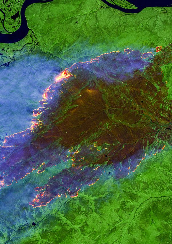
Forest Fire, Sakha Republic, Russia, June 2021 -- Copernicus Sentinel / Sentinel Hub / Pierre Markuse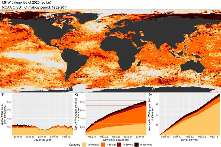

State of the Global Climate 2020
                                   -Provisional report-
Key messages

Concentrations of the major greenhouse gases, CO2, CH4, and N2O, continued to increase in 2019
and 2020.

Despite developing La Niña conditions, global mean temperature in 2020 is on course to be one of
the three warmest on record. The past six years, including 2020, are likely to be the six warmest
years on record.

Sea level has increased throughout the altimeter record, but recently sea level has risen at a higher
rate due partly to increased melting of ice sheets in Greenland and Antarctica. Global mean sea level
in 2020 was similar to that in 2019 and both are consistent with the long-term trend. A small drop in
global sea level in the latter part of 2020 is likely associated with developing La Niña conditions,
similar to the temporary drops associated with previous La Niña events.

Over 80% of the ocean area experienced at least one marine heatwave in 2020 to date. More of the
ocean experienced marine heat waves classified as 'strong' (43%) than 'moderate' (28%).

2019 saw the highest ocean heat content on record and the rate of warming over the past decade
was higher than the long-term average, indicating continued uptake of heat from the radiative
imbalance caused by greenhouse gases.

In the Arctic, the annual minimum sea-ice extent was the second lowest on record and record low
sea-ice extents were observed in the months of July and October. Antarctic sea ice extent remained
close to the long-term average.

The Greenland ice sheet continued to lose mass. Although the surface mass balance was close to the
long-term average, loss of ice due to iceberg calving was at the high end of the 40-year satellite
record. In total, approximately 152 Gt of ice were lost from the ice sheet between September 2019
and August 2020.

Heavy rain and extensive flooding occurred over large parts of Africa and Asia in 2020. Heavy rain
and flooding affected much of the Sahel, the Greater Horn of Africa, the India subcontinent and
neighbouring areas, China, Korea and Japan, and parts of southeast Asia at various times of the year.

With 30 named storms (as of 17 November) the north Atlantic hurricane season had its largest
number of named storms on record with a record number making landfall in the United States of
America. The last storm of the season (to date) Iota, was also the most intense, reaching category 5.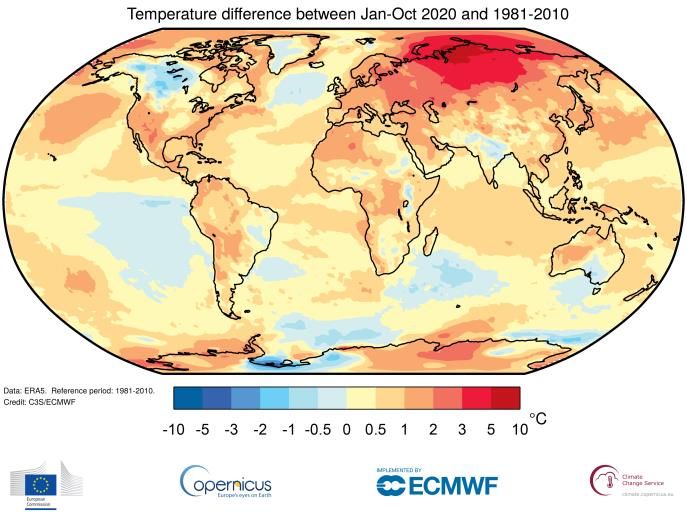

Tropical storm activity in other basins was near or below the long-term mean, although there were
severe impacts.

Severe drought affected many parts of interior South America in 2020, with the worst-affected areas
being northern Argentina, Paraguay and western border areas of Brazil. Estimated agricultural losses
were near US$3 billion in Brazil with additional losses in Argentina, Uruguay and Paraguay.

Climate and weather events have triggered significant population movements and have severely
affected vulnerable people on the move, including in the Pacific region and Central America.

Global climate indicators
Global Climate Indicators1 describe the changing climate, providing a broad view of the climate at a
global scale. They are used to monitor the domains most relevant to climate change, including the
composition of the atmosphere, the energy changes that arise from the accumulation of greenhouse
gases and other factors, as well as the responses of land, ocean and ice. Details on the data sets used
in each section can be found at the end of the report.

Temperature
The global mean temperature for 2020 (January to October) was 1.2 ± 0.1 °C above the 1850–1900
baseline, used as an approximation of pre-industrial levels (Figure 1). 2020 is likely to be one of the
three warmest years on record globally. The WMO assessment is based on five global temperature
datasets (Figure 1). All five of those data sets currently place 2020 as 2nd warmest for the year to
date when compared to equivalent periods in the past (January to October). However, the
difference between the top three years is small and exact rankings for each data set could change
once the year is complete. The spread of the five estimates for the January to October average is
between 1.11 °C and 1.23 °C.

Figure 1: Global annual mean temperature difference from preindustrial conditions (1850–1900). The two reanalyses (ERA5
and JRA-55) are aligned with the in situ datasets (HadCRUT, NOAAGlobalTemp and GISTEMP) over the period 1981–2010.
Data for 2020 run from January to October.

1   https://gcos.wmo.int/en/global-climate-indicators

The warmest year on record to date, 2016, began with an exceptionally strong El Niño, a
phenomenon which contributes to elevated global temperatures. Despite neutral or comparatively
weak El Niño conditions early in 20202, and La Niña conditions developing by late September3, the
warmth of 2020 is comparable to that of 2016.

With 2020 on course to be one of the three warmest years on record, the past six years, 2015–2020,
are likely to be the six warmest on record. The last five-year (2016–2020) and 10-year (2011–2020)
averages are also the warmest on record.

Although the overall warmth of the year is clear, there were variations in temperature anomalies
across the globe (Figure 2). While most land areas were warmer than the long-term (1981-2010)
average, one area in northern Eurasia stands out with temperatures more than five degrees above
average for the first 10 months of the year (see: Sidebar: The Arctic in 2020). Other notable areas of
warmth include limited areas of the southwestern United States, northern and western parts of
South America, parts of Central America, and wider areas of Eurasia including parts of China. For
Europe, it was the warmest January to October period on record. Areas of below-average
temperature on land included western Canada, limited areas of Brazil, northern India and south-
eastern Australia.

Figure 2: Temperature anomalies relative to the 1981-2010 long-term average from the ERA5 reanalysis for January to
October 2020. Credit: Copernicus Climate Change Service, ECMWF.

Greenhouse gases and stratospheric ozone
Atmospheric concentrations of greenhouse gases reflect a balance between emissions from human
activities, natural sources and biospheric and oceanic sinks. Increasing levels of greenhouse gases in
the atmosphere due to human activities are the major driver of climate change since the mid-20th
century.
Global averaged mole fractions of greenhouse gases are calculated from in situ observations from
multiple sites in the Global Atmosphere Watch Programme of WMO and partner networks. These
data are available from the World Data Centre for Greenhouse Gases operated by Japan
Meteorological Agency4.

2 https://origin.cpc.ncep.noaa.gov/products/analysis_monitoring/ensostuff/ONI_v5.php
3 http://www.bom.gov.au/climate/enso/wrap-up/archive/20200929.archive.shtml
4 https://gaw.kishou.go.jp/

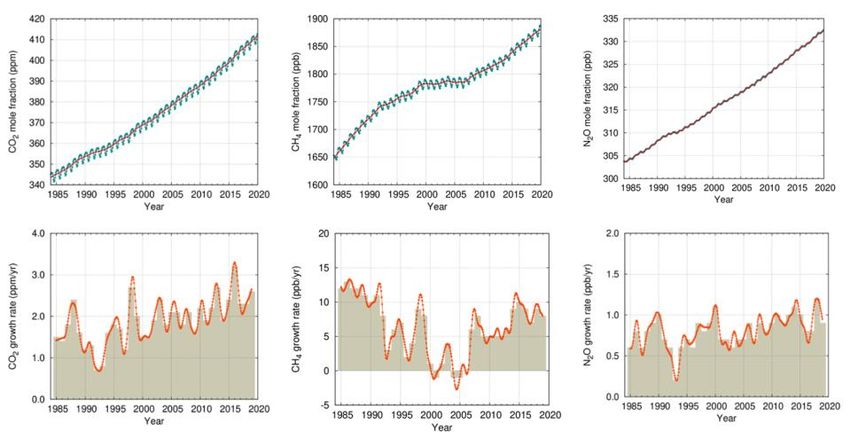
In 2019, greenhouse gas concentrations reached new highs (Figure 3), with globally averaged mole
fractions of carbon dioxide (CO2) at 410.5±0.2 parts per million (ppm), methane (CH4) at 1877±2
parts per billion (ppb) and nitrous oxide (N2O) at 332.0±0.1 ppb. These values constitute,
respectively, 148%, 260% and 123% of pre-industrial (before 1750) levels. The increase in CO2 from
2018 to 2019 (2.6 ppm) was larger than both the increase from 2017 to 2018 (2.3 ppm) and the
average over the last decade (2.37 ppm per year). For CH4, the increase from 2018 to 2019 was
slightly lower than from 2017 to 2018 but still higher than the average over the last decade. For N2O,
the increase from 2018 to 2019 was also lower than that observed from 2017 to 2018 and practically
equal to the average growth rate over the past 10 years.
The temporary reduction in emissions in 2020 related to measures taken in response to COVID-195 is
likely to lead to only a slight decrease in the annual growth rate of CO2 concentration in the
atmosphere, which will be practically indistinguishable from the natural interannual variability
driven largely by the terrestrial biosphere. Real-time data from specific locations, including Mauna
Loa (Hawaii) and Cape Grim (Tasmania) indicate that levels of CO2, CH4 and N2O continued to
increase in 2020.
The IPCC Special Report on Global Warming of 1.5 °C found that limiting warming to 1.5°C above
pre-industrial levels implies reaching net zero CO2 emissions globally around 2050 and concurrent
deep reductions in emissions of non-CO2 forcers.

Figure 3: Top row: Globally averaged mole fraction (measure of concentration), from 1984 to 2019, of CO2 in parts per
million (left), CH4 in parts per billion (centre) and N2O in parts per billion (right). The red line is the monthly mean mole
fraction with the seasonal variations removed; the blue dots and line show the monthly averages. Bottom row: the growth
rates representing increases in successive annual means of mole fractions for CO 2 in parts per million per year are shown as
grey columns (left), CH4 in parts per billion per year (centre) and N2O in parts per billion per year (right) (Source: WMO
Global Atmosphere Watch).

Stratospheric ozone and ozone-depleting gases
Following the success of the Montreal Protocol, use of halons and CFCs has been reported as
discontinued but their levels in the atmosphere continue to be monitored. Because of their long
lifetime, these compounds will remain in the atmosphere for many decades and even if there were
no new emissions, there is still more than enough chlorine and bromine present to cause complete
destruction of ozone in Antarctica from August to December. As a result, the formation of the

5Liu, Z., Ciais, P., Deng, Z. et al. Near-real-time monitoring of global CO 2 emissions reveals the effects of the COVID-19 pandemic. Nat
Commun 11, 5172 (2020). https://doi.org/10.1038/s41467-020-18922-7

Antarctic ozone hole continues to be an annual spring event with year-to-year variation in its size
and depth governed to a large degree by meteorological conditions.

The 2020 ozone hole developed relatively early and continued growing resulting in a large and deep
ozone hole which, as of November 2020, has a larger than average (1979-2019 mean) area of ozone
depletion and lower than average minimum ozone. The ozone hole area reached its maximum area
for 2020 on 20 September at 24.8 million km2, the same area as in 2018. The area of the hole was
closer to the maxima observed in years such as 2015 (28.2 million km2) and 2006 (29.6 million km2)
than 2019 (16.4 million km2) according to an analysis from the National Aeronautics and Space
Administration (NASA).

At the other end of the earth, unusual atmospheric conditions led to ozone concentrations over the
Arctic falling to a record low for the month of March. Unusually weak “wave” events in the upper
atmosphere left the polar vortex relatively undisturbed, preventing mixing of ozone-rich air from
lower latitudes. In addition, the stratospheric polar vortex over the Arctic was strong and this,
combined with consistently very low temperatures, allowed a large area of polar stratospheric
clouds to grow. When the sun rises after the polar winter, it triggers chemical processes in the polar
stratospheric clouds that lead to depletion of ozone. Measurements from weather balloons
indicated ozone depletion surpassing the levels reported in 2011 and together with satellite
observations point to stratospheric ozone levels down to around 205 Dobson Units on March 12,
2020. The typical lowest ozone values previously observed over the Arctic in March are at least 240
Dobson Units.

Ocean
The majority of the excess energy that accumulates in the earth system due to increasing
concentrations of greenhouse gases is taken up by the ocean. The added energy warms the ocean
and the consequent thermal expansion of the water leads to sea level rise. The surface ocean has
warmed more rapidly than the interior and this can be seen in the rise of global mean temperature
and also in the increased incidence of marine heatwaves. As the concentration of CO2 in the
atmosphere rises, so too does the concentration of CO2 in the oceans. This affects ocean chemistry,
lowering the average pH of the water, a process known as ocean acidification. All these changes
have broad range of impacts in the oceans and coastal areas.

Ocean heat content
Increasing human emissions of CO2 and other greenhouse gases cause a positive radiative imbalance
at the top of the atmosphere – the Earth Energy Imbalance (EEI) - which is driving global warming
through an accumulation of energy in the form of heat in the Earth system6,7,8. Ocean Heat Content
(OHC) is a measure of this heat accumulation in the Earth system, as around 90% of it is stored in the
ocean. A positive EEI signals that the Earth’s climate system is still responding to the current forcing9
and that more warming will occur even if the forcing does not increase further10.

Historical measurements of subsurface temperature back to the 1940s mostly rely on shipboard
measurement systems, which constrains the availability of subsurface temperature observations at a

6 Hansen, J. et al. (2011). Earth’s energy imbalance and implications. Atmospheric Chemistry and Physics. https://doi.org/10.5194/acp-11-
13421-2011
7 Rhein, M. et al. 2013. Climate change 2013: The physical science basis.
8
  von Schuckmann, K. et al. (2016). An imperative to monitor Earth’s energy imbalance. In Nature Climate Change.
https://doi.org/10.1038/nclimate2876
9 Hansen, J. et al. (2005). Earth’s Energy Imbalance: Confirmation and Implications. Science, 308(5727), 1431 LP – 1435.

https://doi.org/10.1126/science.1110252
10 Hansen, J. et al. (2017). Young people’s burden: requirement of negative CO2 emissions. Earth Syst. Dynam., 8(3), 577–616.

https://doi.org/10.5194/esd-8-577-2017

global scale and at depth11. With the deployment of the Argo network of autonomous profiling
floats, which first achieved near-global coverage in 2006, it is now possible to routinely measure
OHC changes down to a depth of 2000m 12,13.

Various research groups have developed estimates of global OHC. Although they all rely more or less
on the same database, the estimates show differences arising from the various statistical treatments
of data gaps, the choice of climatology and the approach used to account for instrumental
biases14,15. A concerted effort has been established to provide an international view on the global
evolution of ocean warming 16, and an update to 2019 is shown in Figure 4 and Figure 5. More details
can be found in von Schuckmann et al. (2020).

Figure 4: 1960-2019 ensemble mean time series and ensemble standard deviation (2-sigma, shaded) of global ocean heat
content (OHC) anomalies relative to the 2005-2017 climatology for the 0-300m (grey), 0-700m (blue), 0-2000m (yellow) and
700-2000m depth layer (green). The ensemble mean is an outcome of a concerted international effort, and all products
used are listed at the end of the report and in the legend of Figure 5. Note that values are given for the ocean surface area
between 60°S-60°N, and limited to the 300m bathymetry of each product. Updated from von Schuckmann et al. (2020).

The 0-2000m depth layer of the global ocean continued to warm in 2019 reaching a new record high
(Figure 4), and it is expected that it will continue to warm in the future 17. Heat storage at
intermediate depth (700-2000m) increased at a comparable rate to the 0-300m depth layer, which is
in general agreement among the 15 international OHC estimates (Figure 5). All data sets agree that
ocean warming rates show a particularly strong increase in the past two decades. Moreover, there is
a clear indication that heat sequestration into the ocean below 700m depth took place over the past
six decades linked to an increase of OHC trends over time. Ocean warming rates for the 0-2000m
depth layer reached record rates of 1.2 (0.8) ± 0.2 Wm-2 for the ocean (global) area over the period

11 Abraham, J. P. et al. (2013). A review of global ocean temperature observations: Implications for ocean heat content estimates and
climate change. Reviews of Geophysics, 51(3), 450–483. https://doi.org/10.1002/rog.20022
12 Riser, S. C. et al. (2016). Fifteen years of ocean observations with the global Argo array. Nature Climate Change, 6(2), 145–153.

https://doi.org/10.1038/nclimate2872
13 Roemmich, D. et al. (2019). On the Future of Argo: A Global, Full-Depth, Multi-Disciplinary Array. In Frontiers in Marine Science (Vol. 6, p.

439). https://www.frontiersin.org/article/10.3389/fmars.2019.00439
14 Boyer, T. et al. (2016). Sensitivity of Global Upper-Ocean Heat Content Estimates to Mapping Methods, XBT Bias Corrections, and

Baseline Climatologies. Journal of Climate, 29(13), 4817–4842. https://doi.org/10.1175/JCLI-D-15-0801.1
15 von Schuckmann, K. et al. (2016). An imperative to monitor Earth’s energy imbalance. In Nature Climate Change.

https://doi.org/10.1038/nclimate2876
16 von Schuckmann, K. et al. (2020). Heat stored in the Earth system: Where does the energy go? The GCOS Earth heat inventory team.

Earth Syst. Sci. Data Discuss., 2020, 1–45. https://doi.org/10.5194/essd-2019-255
17 IPCC, 2019: Summary for Policymakers. In: IPCC Special Report on the Ocean and Cryosphere in a Changing Climate[H.-O. Pörtner, D.C.

Roberts, V. Masson-Delmotte, P. Zhai, M. Tignor, E. Poloczanska, K. Mintenbeck, A. Alegría, M. Nicolai, A. Okem, J. Petzold, B. Rama, N.M.
Weyer (eds.)]. In press.

2010-2019. Below 2000m depth, the ocean also warmed albeit at the lower rate of 0.07 ± 0.04 Wm-2
from 1991-201818.

Figure 5: Linear trends of global ocean heat content (OHC) as derived from different temperature products (colors).
References are provided at the end of the report. The ensemble mean and standard deviation (2-sigma) is given in black,
respectively. The shaded areas show trends from different depth layer integrations, i.e. 0-300m (light turquoise), 0-700m
(light blue), 0-2000m (purple) and 700-2000m (light purple). For each integration depth layer, trends are evaluated over
four periods: historical (1960-2019), altimeter era (1993-2019), golden Argo era (2005-2019), and the most recent period
2010-2019. Updated from von Schuckmann et al. (2020).

Sea level
On average, since early 1993, the altimetry-based global mean rate of sea level rise amounts to
3.3 ± 0.3 mm/yr. The rate has also increased over that time. A greater loss of ice mass from the ice
sheets is the main cause of the accelerated rise in the global mean sea level19.

Global mean sea level in 2020 has been similar to that in 2019 (Figure 6, left). A small decrease in the
latter part of 2020 is likely related to La Niña conditions in the tropical Pacific. Interannual changes
of global mean sea level around the long-term trend are correlated with ENSO variability (Figure 6,
right). During La Niña events, such as that in late 2020 and the strong La Niña of 2011, shifts in
rainfall patterns transfer water mass from the ocean to tropical river basins on land, temporarily
reducing global mean sea level. The opposite is observed during El Niño (e.g. the strong 2015-16 El
Niño).

18 Update from Purkey, S. G., and G. C. Johnson, 2010: Warming of Global Abyssal and Deep Southern Ocean Waters between the 1990s
and 2000s: Contributions to Global Heat and Sea Level Rise Budgets. J. Climate, 23, 6336–6351, https://doi.org/10.1175/2010JCLI3682.1.
19 World Climate Research Programme (WCRP) Global Sea Level Budget Group, 2018: Global sea-level budget 1993–present. Earth System

Science Data, 10, 1551–1590, https://doi.org/10.5194/essd-10-1551-2018.

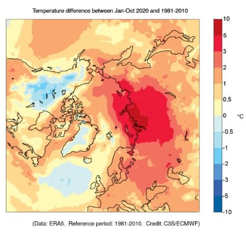
Figure 6: (left) Satellite altimetry-based global mean sea level for January 1993 to October 2020 (last data : 13 October
2020). Data from the ESA climate change Initiative sea level project, from January 1993 to December 2015, (thick black
curve); extended by the Copernicus Marine and Environment Service, CMEMS, until August 2020 (blue curve) and with near
real time altimetry data from the Jason-3 mission beyond August 2020 (red curve). The thin black curve is a quadratic
function that best fits the data. Vertical dashed lines mark the start of each year from 2016 to 2021. (right) Interannual
variability of the (with the quadratic function shown in left-hand panel subtracted) global mean sea level (blue curve) with
the multivariate ENSO index (red curve) superimposed.

At a regional scale, sea level continues to rise non-uniformly. The strongest regional trends over the
period January 1993 to January 2020 are seen in the southern hemisphere: east of Madagascar in
the Indian Ocean; east of New Zealand in the Pacific Ocean; and east of Rio de la Plata/South
America in the south Atlantic. An elongated eastward pattern is also seen in the north Pacific. A
strong pattern that was seen in the western tropical Pacific over the first two decades of the
altimetry record is now fading, suggesting that it was related to short-term variability. Regional sea
level trends are dominated by variations in ocean heat content20. However, in some regions such as
the Arctic, salinity changes due to freshwater input from the melting of ice on land play an important
role.

Marine heatwaves
As with heatwaves on land, extreme heat can affect the near-surface layer of the oceans with a
range of consequences for marine life and dependent communities. Satellite retrievals of sea-
surface temperature can be used to monitor marine heatwaves (MHWs). MHWs are categorised
here as Moderate, Strong, Severe or Extreme (for definitions see Marine heatwave data).

Much of the ocean experienced at least one 'Strong' MHW at some point in 2020 (Figure 7a).
Conspicuously absent are MHWs in the Atlantic Ocean south of Greenland, and in the eastern
equatorial Pacific. The Laptev Sea experienced an ‘Extreme’ MHW from June to October. Sea ice
extent was unusually low in the region and adjacent land areas experienced heatwaves during the
summer. Another important MHW to note in 2020 was the return of the semi-persistent warm
region in the northeast Pacific. This event is similar in scale to the original 'blob' 21,22, which
developed around 2013 with remnants lasting until 201623. Approximately one fifth of the global

20 IPCC, 2019: IPCC Special Report on the Ocean and Cryosphere in a Changing Climate [H.-O. Pörtner, D.C. Roberts, V. Masson-Delmotte,
P. Zhai, M. Tignor, E. Poloczanska, K. Mintenbeck, A. Alegría, M. Nicolai, A. Okem, J. Petzold, B. Rama, N.M. Weyer (eds.)].
21
   Gentemann, C. L. et al., 2017: Satellite sea surface temperatures along the West Coast of the United States during the 2014 –2016
northeast Pacific marine heat wave. Geophysical Research Letters, 4 4, 312– 319, doi:10.1002 /2016GL071039.
22 Di Lorenzo, E. and N. Mantua, 2016: Multi-year persistence of the 2014/15 North Pacific marine heatwave. Nature Climate Change,

6(11), p.1042, doi: 10.1038/nclimate308
23 Schmeisser, L., Bond, N. A., Siedlecki, S. A., & Ackerman, T. P. (2019). The role of clouds and surface heat fluxes in the maintenance of

the 2013–2016 Northeast Pacific Marine heatwave. Journal of Geophysical Research: Atmospheres, 124(20), 10772-10783.

ocean was experiencing a MHW on any given day in 2020 (Figure 7b). This is similar to 2019, but less
than the 2016 peak of 23%. More of the ocean experienced MHWs classified as 'strong' (43%) than
'moderate' (28%). In total, 82% of the ocean experienced at least one MHW during 2020 (to date,
Figure 7c), which is less than both 2019 (84%), and the 2016 peak (88%).

Figure 7: (A) Global map showing the highest MHW category (for definitions see Marine heatwave data) experienced at
each pixel over the course of the year, estimated using the NOAA OISST v2.1 dataset (reference period 1982–2011). Light
grey indicates that no MHWs occurred in a pixel over the entire year; (B) Stacked bar plot showing the percentage of ocean
pixels experiencing an MHW on any given day of the year; (C) Stacked bar plot showing the cumulative percentage of the
ocean that experienced an MHW over the year24.Horizontal lines in this figure show the final percentages for each category
of MHW; (D) Stacked bar plot showing the cumulative number of MHW days averaged over all pixels in the ocean 25(Source:
Robert Schlegel, IMEV).

Ocean acidification
The ocean absorbs around 23% of the annual emissions of anthropogenic CO2 to the atmosphere 26,
thereby helping to alleviate the impacts of climate change on the planet 27. The ecological costs of
this process to the ocean are high, as the CO2 reacts with seawater, lowering its pH, a process known
as ocean acidification. Ocean acidification affects many organisms and ecosystem services,
threatening food security by endangering fisheries and aquaculture. This is particularly a problem in
the polar oceans because of the ocean chemistry of these cold regions. It also affects coastal
protection by weakening coral reefs, which shield coastlines. As the acidity of the ocean increases,
its capacity to absorb CO2 from the atmosphere decreases, hampering the ocean’s role in
moderating climate change. Regular global observation and measurement of ocean acidification is
needed to improve the understanding of its consequences, enable modelling and prediction of
change and variability, and help inform mitigation and adaptation strategies.

Global efforts have been made to collect and compare ocean acidification observation data, which
contribute towards the Sustainable Development Goal (SDG) 14.3 and the associated SDG Indicator
14.3.1: "Average marine acidity (pH) measured at agreed suite of representative sampling stations".

24
   These values are based on when in the year a pixel first experiences its highest MHW category, so no pixel is counted more than once
25 This is taken by finding the cumulative MHW days per pixel for the entire ocean and dividing that by the overall number of ocean pixels
(~690 000).
26 https://library.wmo.int/doc_num.php?explnum_id=10100
27 Le Quéré, C., Andrew, R. M., Friedlingstein, P., Sitch, S., Pongratz, J., Manning, A. C., et al. (2018). Global carbon budget 2017. Earth Syst.

Sci. Data 10, 405–448. doi: 10.5194/essd-10-405-2018

The data are summarised in Figure 8 (left) and show an increase of variability (minimum and
maximum pH values are highlighted) and a decline in average pH at the available observing sites
between 2015 and 2019. The more steady global change (Figure 8, right) estimated from a wider
variety of sources including measurements of other variables, contrasts with the regional and
seasonal variations in ocean carbonate chemistry seen at individual sites. The increasing number of
available data highlight the variability and the trend in ocean acidification and the need for sustained
long-term observations to better characterize the natural variability in ocean carbonate chemistry.

Figure 8: (left) Surface pH values based on ocean acidification data submitted to the 14.3.1 data portal (http://oa.iode.org)
for the time period from 1 January 2010 to 8 January 2020. Grey circles – calculated pH of data submissions (including all
data sets with data for at least two carbonate parameters); blue circles – average annual pH (based on data sets with data
for at least two carbonate parameters); red circles – annual minimum pH; green circles – annual maximum pH. Note that
the number of stations is not constant with time. (right) Global mean surface pH from E.U. Copernicus Marine Service
Information (blue). The shaded area indicates the estimated uncertainty in each estimate.

Cryosphere
The cryosphere is the domain that comprises the frozen parts of the earth. The cryosphere provides
key indicators of the changing climate, but it is one of the most under-sampled domains. The major
cryosphere indicators used in the provisional statement are sea-ice extent and mass balance of the
Greenland ice sheets, both of which can be routinely measured using satellite data. Specific snow
events are covered in the section on High-impact events in 2020. Other cryosphere indicators
including glacier mass balance and permafrost, which are measured in situ, are not covered in the
provisional statement as it takes time to gather and process the data.

Sea ice
In the Arctic, the annual minimum sea-ice extent in September was the second lowest on record
(Figure 9) and record low sea-ice extents were observed in the months of July and October. April and
August extents were among the five lowest in the 42-year satellite data record. Antarctic sea ice
remained close to the long-term average. For more details on the datasets used see Sea ice data.

In the Arctic, the maximum sea-ice extent for the year was reached on 5 March 2020. At just above
15 million km2, this was the 10th or 11th (depending on the data set used) lowest maximum extent on
record28. Sea-ice retreat in late March was mostly in the Bering Sea. In April, the rate of decline was
similar to that of recent years, and the mean sea-ice extent for April was between 2nd and 4th lowest,
effectively tied with 2016, 2017, and 2018.

Record high temperatures north of the Arctic Circle in Siberia (see Sidebar: The Arctic in 2020)
triggered an acceleration of sea-ice melt in the East Siberian and Laptev Seas, which continued well

28   http://nsidc.org/arcticseaicenews/2020/03/

into July. Sea-ice extent for July was the lowest on record29 (7.28 million km2). The sea-ice retreat in
the Laptev Sea was the earliest observed in the satellite era. Towards the end of July, a cyclone
entered the Beaufort Sea and spread the sea-ice out, temporarily slowing the decrease of the ice
extent. In mid-August, the area affected by the cyclone melted rapidly which, combined with the
sustained melt in the East Siberian and Laptev Seas, made the August extent the 2nd or 3rd lowest on
record.

The 2020 Arctic sea-ice extent minimum was observed on 15 September at 3.74 million km2, marking
only the second time on record that the Arctic sea-ice extent shrank to less than 4 million km2. Only
2012 had a lower minimum extent at 3.39 million km2. Vast areas of open ocean were observed in
the Chukchi, East Siberian, Laptev, and Beaufort Seas, notwithstanding a tongue of multi-year ice
that survived the 2020 melt season in the Beaufort Sea30 (Figure 10).

Refreeze was slow in late September and October in the Laptev and East Siberian Seas, probably due
to the accumulated heat in the upper ocean since the early retreat in late June. Arctic sea-ice extent
was the lowest on record for October.

In the Antarctic, the minimum sea-ice extent was observed later than usual, on 2 March, at
2.73 million km2. Sea-ice extent was close to the climatological average for most of the year and was
above average in September and October. The maximum extent was reached on 28 September at
18.95 million km2.

Figure 9: Sea-ice extent difference from the 1981-2010 average in the Arctic (left) and Antarctic (right) for the months with
maximum ice cover (Arctic: March, Antarctic: September) and minimum ice cover (Arctic: September, Antarctic: February).
Data from EUMETSAT OSI SAF v2p1 (Lavergne et al., 2019) and NSIDC v3 (Fetterer et al., 2017).

29   https://cryo.met.no/en/arctic-seaice-summer-2020
30   https://cryo.met.no/en/arctic-seaice-september-2020

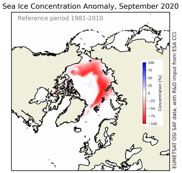
Figure 10: Sea Ice Concentration anomaly against the 1981-2010 period for the Arctic (EUMETSAT OSI SAF v2p1 data, with
R&D input from ESA CCI). Sea-ice concentration is a parameter used to describe how densely the sea ice is packed. It is
expressed by a continuous scale from complete ice cover (100%) to an open ocean with no ice (0%).

Greenland Ice Sheet
Despite the exceptional warmth in large parts of the Arctic, in particular the very unusual
temperatures that were observed in eastern Siberia since February 2020, temperatures over
Greenland were close to the long-term mean (see Figure 2). The ice sheet ended the September
2019 to August 2020 season with an overall loss of 152 Gt (gigatons) of ice from surface melting, the
discharge of icebergs and from melting of glacier tongues by warm ocean water (Figure 11). This
means that the ice sheet continued to lose ice, though at a slower rate than seen in 2019 (which saw
a loss of 329 Gt).

Changes in the mass of the Greenland ice sheet reflect the combined effects of surface mass balance
(SMB) – defined as the difference between snowfall and run-off from the ice sheet, which is always
positive at the end of the year – and mass losses at the periphery from the calving of icebergs and
the melting of glacier tongues that meet the ocean. The 2019-20 Greenland SMB was +349 Gt of ice,
which is close to the 40-year average of +341 Gt. However, ice loss due to iceberg calving was at the
high end of the 40-year satellite record. The Greenland SMB record is now four decades long and,
although it varies from one year to another, there has been an overall decline in the average SMB
over time (Figure 11). In the 1980s and 1990s, the average SMB gain was about +416 Gt/year. It fell
to +270 Gt in the 2000s and +260 Gt in the 2010s.

The GRACE satellites and the follow-up mission GRACE-FO measure the tiny change of the
gravitational force due to changes in the amount of ice. This gives us an independent measure of the
total mass balance. Based on this data, it can be seen that the Greenland ice sheet has lost about
4200 Gt from April 2002 to August 2019, which contributed to a sea level rise of slightly more than 1
cm. This is in good agreement with the mass balance from SMB and discharge, which during the
same period was 4261 Gt.

The 2019-20 melt season on the ice sheet started on 22 June, 10 days later than the 1981-2020
average. As in previous years, there were losses along the Greenlandic west coast and gains in the
east. In mid-August, unusually large storms brought four times the normal monthly precipitation to
western Greenland, most of which fell as snow that temporarily stopped the net loss of ice and was

decisive in reducing the amount of melt, quite different from the previous year 2018-19 with
extended high pressure periods and large amounts of sunshine which significantly increased the
amount of melt in summer.

Figure 11: Components of the total mass balance of the Greenland Ice Sheet 1986-2020. Blue: Surface mass balance31,
green: discharge, red: total mass balance, the sum of Surface Mass Balance and discharge32.

Drivers of short-term climate variability
There are many different natural phenomena, often referred to as climate patterns or climate
modes, that affect weather at timescales ranging from days to several months. Surface
temperatures change relatively slowly over the ocean, so recurring patterns in sea surface
temperature can be used to understand and, in some cases, predict the more rapidly changing
patterns of weather over land on seasonal time scales. Similarly, albeit at a faster rate, known
pressure changes in the atmosphere can help explain certain regional weather patterns.

In 2020, the El Niño–Southern Oscillation, a phenomenon measured by both the oceans and the
atmosphere, and the Arctic Oscillation, an atmospheric phenomenon, each contributed to specific
weather events in different parts of the world. The Indian Ocean Dipole, which played a key role in
the events of 2019 was near-neutral for much of 2020.

El Niño Southern Oscillation (ENSO)
ENSO is one of the most important drivers of year-to-year variability in weather patterns around the
world. It is linked to hazards such as heavy rains, floods, and drought. El Niño, characterised by
higher-than-average sea surface temperatures in the eastern Pacific and a weakening of the trade
winds, typically has a warming influence on global temperatures. La Niña, which is characterised by
below-average sea-surface temperatures in the central and eastern Pacific and a strengthening of
the trade winds, has the opposite effect.

Sea-surface temperatures at the end of 2019 were close to or exceeded El Niño thresholds in the
Niño 3.4 region33. These persisted into the early months of 2020, but the event did not strengthen

31 http://polarportal.dk/en/greenland/surface-conditions/.
32 Mankoff, K.D. et al. (2020) Greenland Ice Sheet solid ice discharge from 1986 through March 2020 Earth Syst. Sci. Data, 12, 1367–1383,
https://doi.org/10.5194/essd-12-1367-2020
33 https://origin.cpc.ncep.noaa.gov/products/analysis_monitoring/ensostuff/ONI_v5.php

and sea surface temperature anomalies in the eastern Pacific fell in March. After a six-month period
of neutral conditions – that is, sea surface temperatures within 0.5 °C of normal – the cool-phase, La
Niña, developed in August and strengthened in October, although it was technically still defined as
weak (0.5–1.0°C below normal). The atmosphere also responded with stronger than average trade
winds, indicating a coupling with the sea surface temperatures. La Niña conditions are associated
with above-average hurricane activity in the North Atlantic, which has experienced a record number
of named tropical storms during its 2020 hurricane season. La Niña is expected to persist through
the first quarter of 202134.

Arctic Oscillation (AO)
The AO is a large-scale atmospheric pattern that influences weather throughout the Northern
Hemisphere. The positive phase is characterised by lower-than-average air pressure over the Arctic
and higher-than-average pressure over the northern Pacific and Atlantic Oceans. The jet stream is
parallel to the lines of latitude and farther north than average, locking up cold Arctic air, and storms
can be shifted northward of their usual paths. The mid-latitudes of North America, Europe, Siberia,
and East Asia generally see fewer cold air outbreaks than usual during the positive phase of the AO.
A negative AO has the opposite effect, associated with a more meandering jet stream and cold air
spilling south into the mid-latitudes.

The AO was strongly positive during the Northern Hemisphere 2019-20 winter and was the strongest
in February since January 1993. This contributed to the warmest winter on record for Asia and
Europe and the sixth warmest for the contiguous United States, contrasted by Alaska’s coldest
winter in more than two decades. Additionally, the positive winter phase of the Arctic Oscillation has
been linked to low sea ice extent the following summer (Rigor et al. 200235). See the section on Sea
ice.

Sidebar: The Arctic in 2020
The Arctic is undergoing drastic changes as the global temperature increases. Since the mid-1980s,
Arctic surface air temperatures have warmed at least twice as fast as the global average, while sea
ice, the Greenland ice sheet and glaciers have declined over the same period and permafrost
temperatures have increased. This has potentially large implications not only for Arctic ecosystems,
but also for the global climate through various feedbacks36.

For the first 10 months of 2020, the Arctic stands out as the region with the largest temperature
deviations from the long-term average. Contrasting conditions of ice, heat and wildfires were seen in
the eastern and western Arctic (Figure 12). A strongly positive phase of the Arctic Oscillation during
Winter 2019-20 set the scene early in the year, with higher than average temperatures across
Europe and Asia and well-below average temperatures in Alaska, a pattern which persisted through
much of the year.

In a large region of the Siberian Arctic, temperature anomalies for January to October were more
than 3 °C, and in its central coastal parts more than 5 °C, above average (Figure 14). A preliminary
record temperature was set for north of the Arctic Circle, of 38 °C on 20 June in Verkhoyansk 37,

34 https://ane4bf-datap1.s3-eu-west-1.amazonaws.com/wmocms/s3fs-public/ckeditor/files/El-Nino-La-Nina-Update-October-2020-
en.pdf?UGaW3HcT_wYatEuK8tCOdCqjq4Qr4kSb
35 Rigor, I. G., Wallace, J. M., & Colony, R. L. (2002). Response of sea ice to the Arctic Oscillation. Journal of Climate, 15(18), 2648–2663.

https://doi.org/10.1175/1520-0442(2002)0152.0.CO;2

36 IPCC, 2019: IPCC Special Report on the Ocean and Cryosphere in a Changing Climate [H.-O. Pörtner, D.C. Roberts, V. Masson-Delmotte,
P. Zhai, M. Tignor, E. Poloczanska, K. Mintenbeck, A. Alegría, M. Nicolai, A. Okem, J. Petzold, B. Rama, N.M. Weyer (eds.)].
37 https://public.wmo.int/en/media/news/reported-new-record-temperature-of-38%C2%B0c-north-of-arctic-circle

during a prolonged heatwave. Heatwaves and heat records were also observed in other parts of the
Arctic (see High-impact events in 2020) and extreme heat was not confined to the land only. An
“extreme” marine heatwave affected large areas of the Arctic Ocean north of Eurasia (see Figure 7).
Sea ice in the Laptev Sea, offshore from the area of highest temperature anomalies on land, was
unusually low through the summer and autumn. Indeed, sea ice extent was particularly low along
the Siberian coastline, with the Northern Sea Route ice-free or close to ice free from July to October.

Although the Arctic was predominantly warmer than average for this period, some regions, including
parts of Alaska and Greenland, saw close-to or below-average temperatures. As a result, the 2019-20
surface mass balance for Greenland was close to the 40-year average. Nevertheless, the decline of
the Greenland ice sheet continued during the 2019-20 season, but the loss was below the typical
amounts seen during the last decade (see Cryosphere). Sea ice conditions along the Canadian
archipelago were close to average at the September minimum and the western passage remained
closed38.

The wildfire season in the Arctic during 2020 has been particularly active, but with large regional
differences. The region north of the Arctic circle saw the most active wildfire season in an 18-year
data record, as estimated in terms of fire radiative power and CO2 emissions released from fires. The
main activity was concentrated in the eastern Siberian Arctic, which was also drier than average.
Regional reports39 for eastern Siberia indicate that the forest fire season started earlier than
average, and for some regions ended later, resulting in long-term damage to local ecosystems.
Alaska, as well as Yukon and the Northwest Territories reported fire activity that was well below
average.

38 Arctic Climate Forum https://arctic-rcc.org/sites/arctic-rcc.org/files/presentations/acf-fall-2020/2%20-%20Day%202%20-%20ACF-
6_Arctic_summary_MJJAS_2020_v2.pdf
39 https://arctic-rcc.org/sites/arctic-rcc.org/files/presentations/acf-fall-2020/3%20-%20Day%201-

%20ACF%20October%202020%20Regional%20Overview%20Summary%20with%20extremes%20-281020.pdf

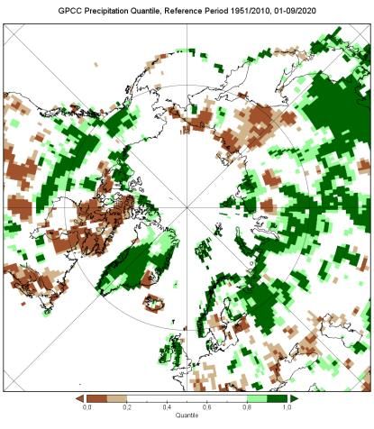
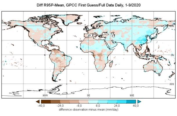
Figure 12: (top left) Temperature anomalies for the Arctic relative to the 1981-2010 long-term average from the ERA5
reanalysis for January to October 2020. Credit: Copernicus Climate Change Service, ECMWF. (top right) Fire Radiative
Power, a measure of heat output from wildfires, in the Arctic Circle between June and August 2020. Credit: Copernicus
Atmosphere Monitoring Service, ECMWF (bottom left) Total precipitation in Jan-Sep 2020, expressed as a percentile of the
1951–2010 reference period, for areas that would have been in the driest 20% (brown) and wettest 20% (green) of years
during the reference period, with darker shades of brown and green indicating the driest and wettest 10%, respectively
Credit: Global Precipitation Climatology Centre (GPCC). (bottom right) sea-ice concentration anomaly for September 2020.
Credit: EUMETSAT OSI SAF data with R&D input from ESA CCI.

High-impact events in 2020
Although understanding broad-scale changes in the climate is important, the most acute impacts of
weather and climate are often felt during extreme meteorological events such as heavy rain and
snow, droughts, heatwaves, cold waves, and storms, including tropical storms. These can lead to or
exacerbate other high-impact events such as flooding, landslides, wildfires and avalanches.

A year of widespread flooding, especially in Africa and Asia
Very extensive flooding occurred over large parts of Africa in 2020. Rainfall was well above average
in most of the Greater Horn of Africa during the March-May “long rains” season, following a similarly
wet season in October-December 2019. This was followed by above-average rainfall across the vast
majority of the Sahel region, from Senegal to Sudan, during the summer monsoon (Figure 13).
Flooding was extensive across many parts of the region, although Sudan and Kenya were the worst-
affected with 285 deaths reported in Kenya40, and 155 deaths and over 800,000 people affected in

40   EM-DAT.

Sudan41, along with further indirect impacts from disease. Countries reporting loss of life or
significant displacement of populations included Sudan, South Sudan, Ethiopia, Somalia, Kenya,
Uganda, Chad, Nigeria, Niger, Benin, Togo, Senegal, Côte d’Ivoire, Cameroon and Burkina Faso. Many
lakes and rivers reached record high levels, including Lake Victoria in May, and the Niger River at
Niamey and the Blue Nile at Khartoum in September.

Figure 13: (left) Total precipitation in Jan-Sep 2020, expressed as a percentile of the 1951–2010 reference period, for areas
that would have been in the driest 20% (brown) and wettest 20% (green) of years during the reference period, with darker
shades of brown and green indicating the driest and wettest 10%, respectively (Source: Global Precipitation Climatology
Centre (GPCC), Deutscher Wetterdienst, Germany). (right) Difference between the observed 95th percentile of daily
precipitation total in Jan-Sep 2020 and the long-term mean based on 1982-2016 (full year). Blue indicate more extreme
daily precipitation events and brown less than the long-term means.

India had one of its two wettest monsoon seasons since 1994, with nationally-averaged rainfall for
June to September 9% above the long-term average. Heavy rain, flooding and landslides also
affected surrounding countries. August was the wettest month on record for Pakistan, and 231 mm
of rain fell on 28 August at Karachi-Faisal, the highest daily total on record in the Karachi area. More
than 2000 deaths were reported during the season in India, Pakistan, Nepal, Bangladesh,
Afghanistan and Myanmar42, including 145 deaths in flash flooding in Afghanistan in late August, and
166 deaths in a landslide at a mine in Myanmar in early July, following heavy rain.

Persistent high rainfall in the Yangtze River catchment in China in the monsoon season also caused
severe flooding. The June-July period was particularly wet and floods affected the Yangtze and its
tributaries, with the Three Gorges Dam discharging water at its maximum capacity. Reported
economic losses exceeded US$15 billion, and at least 279 deaths were reported during the period. It
was also a very wet summer monsoon season over the Korean Peninsula, with the Republic of Korea
experiencing its third-wettest summer, and parts of western Japan were affected by significant
flooding in July.

Parts of southeast Asia experienced severe flooding in October and November. The worst affected
area was central Vietnam, where heavy rains typical of the arrival of the northeast monsoon were
exacerbated by a succession of tropical cyclones and depressions, with eight making landfall in less
than five weeks. Hué received over 1800 mm of rain in the week from 7 to 13 October, and a total of
2615 mm for the month of October. The flooding also extended further west into Cambodia.

Other regions to experience significant loss of life in floods (mostly flash floods associated with
extreme local rainfall) included Indonesia in January, Brazil in January and March, the Democratic

41   Reliefweb, Situation Report, Sudan, 13 November 2020.
42   EM-DAT.

Republic of the Congo and Rwanda in April and May, and Yemen in July. Jakarta had its wettest day
since 1996 with 377 mm at Halim Airport on 1 January, and Belo Horizonte its wettest day on record
with 172 mm on 24 January. Khombole in Senegal had its wettest day on record with 225.8 mm on 5
September.

Heatwaves, drought and wildfire
Severe drought affected many parts of interior South America in 2020, with the worst-affected areas
being northern Argentina, Paraguay and western border areas of Brazil. It was the second-driest
January-August period on record for the northeast region of Argentina, whilst rainfall for the period
was also far below average in Paraguay. Estimated agricultural losses were near US$3 billion in Brazil
with additional losses in Argentina, Uruguay and Paraguay. Peru also experienced drought conditions
between January and March, mainly in the north of the country43. As the drought continued, a major
heatwave stretched across the region in late September and early October, extending east and north
to cover much of interior Brazil. It reached 44.6 °C on 5 October at Nova Maringá and Água Clara,
whilst individual locations which had their hottest day on record included Cuiaba, Curitiba, Belo
Horizonte and Asuncion. There was significant wildfire activity across all three countries from mid-
year onwards, with some of the most significant wildfires occurring in the Pantanal wetlands in
western Brazil.

2020 has been an exceptionally warm year in most of Russia, especially Siberia. Temperatures
averaged over Russia for January to August were 3.7 °C above average, 1.5 °C above the previous
record set in 2007. In parts of northern Siberia the year to date has been 5 °C or more above
average. The heat culminated in late June, when it reached 38.0 °C at Verkhoyansk on the 20th,
provisionally the highest known temperature anywhere north of the Arctic Circle. Abnormal warmth
also extended to other parts of the high Arctic outside Russia, with temperatures reaching records
on 25 July of 21.9 °C at Eureka (Canada), and 21.7 °C at Svalbard Airport. Extensive wildfires occurred
through many parts of northern Siberia, contributing to record high wildfire-related carbon
emissions during the Arctic summer44, and the warmth contributed to exceptionally early sea ice
retreat along the Russian Arctic coast.

A number of exceptionally large wildfires, including the largest fires ever recorded in the states of
California and Colorado, occurred in the western United States in late summer and autumn.
Widespread drought conditions through the western half of the country, particularly the interior
southwest, contributed to the fires, as did a very weak summer monsoon. July to September were
the hottest and driest on record for the southwest. Abnormal lightning activity in coastal California
in mid-August also ignited many fires. The most destructive fires were in California and western
Oregon, with over 8,500 structures destroyed in California and 2,000 in Oregon; 41 deaths in total
were attributed to the fires across multiple states 45. There were also a number of episodes of
extreme heat. Death Valley reached 54.4 °C on 16 August, the highest known temperature in the
world in at least the last 80 years, whilst 49.4 °C on 6 September at Woodland Hills was a record for
greater Los Angeles.

Major wildfires in eastern Australia which had burned through the later part of 2019 continued into
early 2020, before finally being controlled after heavy rain in early February. Drought conditions
which had prevailed since early 2017 eased from January onwards, but there were a number of
episodes of extreme heat in early 2020. Penrith in western Sydney reached 48.9 °C on 4 January, the

43 https://cdn.www.gob.pe/uploads/document/file/1325635/INFORME-LLUVIAS-2019-2020%20FINAL-29-09-2020v2.pdf
44 Copernicus Atmosphere Monitoring Service.
45 NCEI Billion-Dollar Weather and Climate Disasters. https://www.ncdc.noaa.gov/billions/events/US/2020

highest observed in an Australian metropolitan area, whilst Canberra, which set monthly records in
all three summer months, reached a new high of 44.0 °C on the same day. Severe smoke pollution
also affected many parts of southeastern Australia in the early part of 2020. A number of stations in
New Zealand reported their longest dry spell on record between late December 2019 and late
February 2020.

A major heatwave affected the Caribbean region and Mexico in April. Temperatures reached 39.7 °C
at Veguitas on 12 April, a national record for Cuba, whilst Havana also had its hottest day with
38.5 °C. In eastern Mexico temperatures exceeded 45 °C at a number of locations, reaching as high
as 48.8 °C at Gallinas on 12 April, whilst very high readings in Central America included 41.2 °C at San
Agustin Acasaguatlan (Guatemala). Further extreme heat in September saw national or territorial
records set for Dominica, Grenada and Puerto Rico.

Dry conditions affected parts of north-central Europe during spring and summer 2020, although
generally not to the same extent as in 2018 or 2019. April was especially dry, with Romania and
Belarus having their driest April on record and Germany and the Czech Republic their second driest,
while Geneva, Switzerland had a record 43-day dry spell from 13 March to 24 April. There was also a
significant heatwave in western Europe in August. Whilst it was generally not as intense as those of
2019 (except locally on the northern coast of France), many locations, particularly in northern
France, reached temperatures which ranked second behind the 2019 heatwaves, and De Bilt
(Netherlands) had a record eight consecutive days above 30 °C. In early September the focus of
extreme heat shifted to the eastern Mediterranean, with all-time records at locations including
Jerusalem (42.7 °C) and Eilat (48.9 °C) on 4 September, following a late July heatwave in the Middle
East in which Kuwait Airport reached 52.1 °C and Baghdad 51.8 °C.

It was a very hot summer in parts of east Asia. Hamamatsu (41.1 °C) equalled Japan’s national record
on 17 August, and Taipei had its hottest day on record with 39.7 °C on 24 July. Hong Kong had a
record run of 13 consecutive hot nights, with a daily minimum temperature of 28 °C or above, from
19 June to 1 July, followed by 11 consecutive hot nights from 5 to 15 July.

Long-term drought continued to persist in parts of southern Africa, particularly the Northern and
Eastern Cape Provinces of South Africa, although heavy winter rains saw water storages reach full
capacity in Cape Town, continuing the recovery from extreme drought, which peaked in 2018.
Rainfall during the 2019-20 summer rainy season in interior southern Africa was locally heavy, but
long-term drought persisted in some areas.

Extreme cold and snow
North America’s most significant snowstorm of the 2019-20 winter occurred on 17-18 January in
Newfoundland. St. John’s received 75 cm of snow, including a record daily snowfall, and wind gusts
of 126 km/h. Later in the year, there were two extreme early-season cold episodes in autumn. In the
second week of September, widespread snowfalls occurred in lowland Colorado, including Denver,
where a September record high of 38.3 °C had been set only three days earlier, on 5 September.
Later, in October, a major cold outbreak brought exceptionally low temperatures and winter
precipitation across a broad region of the Rocky Mountains and central states. A damaging ice storm
in Oklahoma City saw power outages which lasted for days across more than half the city, whilst
further north, Potomac, Montana reached −33.9 °C on 25 October, the earliest autumn date on
which temperatures had fallen below −30 °C at a climate station anywhere in the United States
(excluding Alaska).

The extremely wet and warm winter in northern Europe resulted in exceptionally low snow cover in
many places – Helsinki experienced a record low number of snow-covered days, breaking the
previous record by a wide margin – but in far northern Europe, where temperatures were above
average but still cold enough for snow, the snowpack was exceptionally heavy. At Sodankylä
(Finland), the snowpack reached record depths in mid-April. A cold May led to a delayed melt with
some cover persisting into June, while flooding occurred in late May and early June with the spring
melt. Rain-on-snow events prevented some reindeer herds from reaching feed.

It was a cold winter in southern South America. Tierra del Fuego had its most significant cold spell
since 1995 in late June and early July, with Rio Grande recording a maximum of −8.8 °C and
minimum of −16.5 °C on 1 July. Paraguay saw record minimum temperatures for August in a number
of places. Snow cover in Patagonia was the second-most extensive since 2000 and sea ice formed
along parts of the Tierra del Fuego coast. Some stock losses were reported. In August, a cold wave in
the north of Peru’s Amazonia saw temperatures at Caballacocha reach 12.8°C, the lowest
temperature recorded there since 1975.

Abnormal low-elevation snowfalls occurred in Tasmania in early August. On 4 August, snow settled
to sea level in Launceston, the city’s most significant snowfall since 1921. Liawenee, in the central
highlands, reached −14.2 °C on 7 August, a Tasmanian record low.

Tropical storms and an exceptionally active North Atlantic hurricane season
The number of tropical cyclones globally was above average in 2020, with 96 named tropical storms
(to 17 November) in the 2020 Northern Hemisphere and 2019-20 Southern Hemisphere seasons.
The North Atlantic region had a very active season, with 30 tropical cyclones as of 17 November,
more than double the long-term average and breaking the record for a full season, set in 2005. Most
other basins had cyclone numbers near or slightly below average.

The Accumulated Cyclone Energy (ACE) index, which integrates cyclone intensity and longevity, was
well below average in all basins except the North Atlantic and North Indian Oceans, with the
Northwest Pacific about 50% below the long-term average. Whilst ACE seasonal values for the North
Atlantic were above average, they were well short of seasonal records.

The exceptionally active North Atlantic season resulted in a large number of landfalls. 12 systems
made landfall in the United States, breaking the previous record of nine; five of them in the state of
Louisiana. The most severe impacts of the season in the United States came from Laura, which
reached category 4 intensity and made landfall on 27 August near Lake Charles in western Louisiana,
with extensive wind and storm surge damage. Laura was also associated with extensive flood
damage in Haiti and the Dominican Republic in its developing phase. 77 deaths and US$14 billion in
economic losses46 were attributed to the storm across the three countries. Later in the season, two
major hurricanes made landfall in rapid succession in Central America. Hurricane Eta made landfall
as a category 4 system on the east coast of Nicaragua on 3 November, causing severe flooding in the
region as it moved slowly across Nicaragua, Honduras and Guatemala. Eta moved offshore on 6
November and re-intensified to a tropical storm, making further landfalls in Cuba and on the Florida
Keys. Iota was even stronger, becoming the season’s first category 5 system off the Nicaraguan coast
on 16 November.

46   NCEI Billion-Dollar Weather and Climate Disasters (economic losses), EM-DAT (deaths).