Statistical analysis of chemical computational
←
→
Page content transcription
If your browser does not render page correctly, please read the page content below
Statistical analysis of chemical computational
         systems with M ULTI V E S TA and A LCHEMIST

    Abstract—The chemical-oriented approach is an emerging            To sum up, the simulator has been enriched with: (1) a
paradigm for programming the behaviour of densely distributed         language (M ULTI Q UATE X) to compactly and cleanly express
and context-aware devices (e.g. in ecosystems of displays tailored    systems properties, decoupled from the model specification;
to crowd steering, or to obtain profile-based coordinated visual-     (2) the automatized estimation of the expected values of
ization). Typically, the evolution of such systems cannot be easily   M ULTI Q UATE X expressions with respect to n independent
predicted, thus making of paramount importance the availability
of techniques and tools supporting prior-to-deployment analysis.
                                                                      simulations, with n large enough to respect a user-specified
Exact analysis techniques do not scale well when the complexity       confidence interval; (3) the generation of gnuplot input files to
of systems grows: as a consequence, approximated techniques           visualize the obtained results; (4) a client-server architecture
based on simulation assumed a relevant role. This work presents       to distribute simulations. The tool is validated by analyzing a
a new simulation-based distributed tool addressing the statistical    crowd steering model reminiscent of the one presented in [12].
analysis of such a kind of systems, which has been obtained
by chaining two existing tools: M ULTI V E S TA and A LCHEMIST.          Synopsis. §II introduces A LCHEMIST and describes the
The former is a recently proposed lightweight tool which allows       crowd steering scenario, while §III outlines the main features
to enrich existing discrete event simulators with distributed         of M ULTI V E S TA. Then §IV discusses the integration of the
statistical analysis capabilities, while the latter is an efficient   two tools, while §V validates the obtained tool. Finally, §VI
simulator for chemical-oriented computational systems. The tool       reports some concluding remarks and future works.
is validated against a crowd steering scenario, and insights on
the performance are provided by discussing how these scale                                         II.       A LCHEMIST
distributing the analysis tasks on a multi-core architecture.
                                                                          A LCHEMIST is a simulator targeting chemical-oriented
                                                                      computational systems. It is aimed at bridging the gap between:
                      I.   I NTRODUCTION                              (1) tools that provide programming/specification languages
    The number of intercommunicating devices spread around            devoted to ease the construction of the simulation process,
the world is constantly increasing: sensors, phones, tablets,         especially targeting computing and social simulation (e.g. as in
eyeglasses and many other everyday objects are carrying more          the case of simulation based on multi-agents [8], [13]–[16]);
and more computational and communicational capabilities.              and (2) tools that stick to foundational languages, which
Such a computationally dense environment called for new               typically offer better performance, mostly used in biology-
programming approaches, many of them inspired by natural              oriented applications [17]–[20]. A LCHEMIST extends the basic
systems, e.g. biological [1], [2], physical [3] and chemical [4],     computational model of chemical reactions – still retaining its
[5]. In all of them, the overall system’s behaviour emerges from      high performance – aiming at easing its applicability to complex
local, simple and probabilistic interactions among the devices        situated computational systems (following the chemical-oriented
composing the computational continuum. For this reason, most          abstractions studied in [4]). In particular, A LCHEMIST is based
of the work in literature focuses on modelling single devices.        on an optimised version of the Gillespie’s SSA [21] called Next
When this reductionist point of view is adopted, a difficult task     Reaction Method [22], properly extended with the possibility
in the development methodology is to assert system properties:        to deal with a mobile and dynamic “environment” (adding/re-
the system’s evolution can not be easily predicted and thus           moving reactions, data-items and topological connections). The
multiple simulations runs are performed [6]–[9]. Obvious              underlying meta-model and simulation framework are built
questions accompany these procedures: how reliable are the            to be as generic as possible, and as such they can have a
obtained values? How is the number of performed simulation            wide range of applications like pervasive computing, social
chosen? And how many simulations are required in order to             interactions and computational biology [23].
state system properties with a certain degree of confidence?              A detailed description of the simulator’s meta-model and
Moreover, there is frequently a lack of decoupling between the        its engine’s internals are out of the scope of this work. The
model specification and the definition of the system’s properties     interested reader can find a deeper insight in [10]. A LCHEMIST
of interest: they are often embedded in the model, and their          is written in Java and is still actively developed. It currently
values are obtained via logging during the simulation process.        consists of about 630 classes for about 100’000 lines of code,
    This work presents a new tool obtained chaining                   and it is released 1 as open source (GPL licensed).
A LCHEMIST [10], an efficient state-of-the-art simulator
for chemical-oriented computational systems, with M ULTI -            A. A crowd steering scenario
V E S TA [11], a recently proposed lightweight tool which allows         Our reference scenario, depicted in Figure 1, consists of
to enrich existing discrete event simulators with distributed         a hall of 20 × 10 meters on whose floor a regular grid of
statistical analysis capabilities. The result is thus a statistical
analysis tool tailored to chemical-inspired pervasive systems.          1 http://alchemist.apice.unibo.it.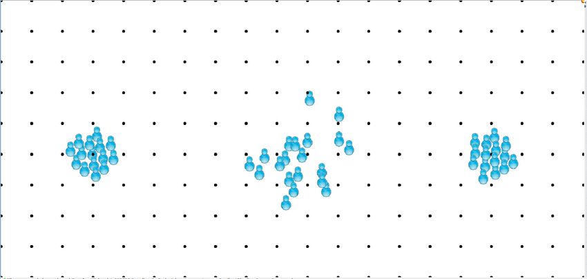
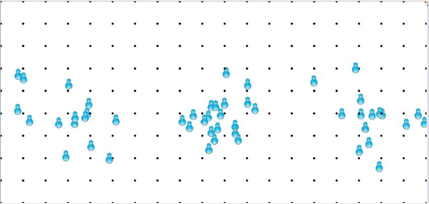
Fig. 1.   Three snapshots of the reference scenario showing: the system at the initial stage (left), an intermediate state (centre), and the final situation (right).

200 computationally enabled sensors is deployed. In the hall,                         dynamicity, gradients must then provide a feature commonly
three groups of 15 people each are located. One group, on                             identified as self-healing ability. Fortunately, nice algorithms
the left, wants to get to a point of interest (POI) on the right.                     have already been proposed for self-healing gradients [25],
Another group, on the right, desires to get to a POI on the left.                     [26]. Similar manipulations of self-healing gradients have been
Finally, a third group stands in the centre of the hall. Each                         used in other works, by aggregating multiple gradients [27],
person is equipped with a smartphone. Devices (i.e. sensors                           by combining them with local information [28], or both [29].
and smartphones) are able to communicate with devices within                             2) The pedestrians model: A LCHEMIST provides a realistic
their communication range (1.5 meters). Sensors can count                             pedestrian model, based primarily on [30]. We relied on such
the people in such range, while smartphones provide real time                         model to obtain a realistic physical interaction among people.
suggestions to the user about the direction to be taken. Users are                    A deep analysis of this model is out of the scope of this work.
supposed to follow the advices of their smartphone whenever
possible, however, a pedestrian model that makes them subject                             3) Implementation with a chemical metaphor: In this
to physical interactions is used. Such model also includes the                        scenario we propose a solution relying on the SAPERE concepts
social desire of not breaking the group, which may lead the                           of “live semantic annotation” (LSA) and “eco-law” [4]. LSAs
users to choose a direction different from the suggested one.                         are “semantic annotations” in the sense that they can carry
                                                                                      semantic information, and they are “live” in the sense that they
    In such a scenario, we want to deploy a fully distributed                         are in charge of reflecting the perceived status of the world
crowd steering system, in which the sensors automatically build                       for every device. All the data in the system are encoded as
optimal paths, so that from whichever location in the hall, each                      LSA, for instance in the considered scenario both the spatial
user can move towards the desired direction. We also want to                          gradient and the crowd level detection are reified in form of
employ the local real time information about the number of                            LSAs. The eco-laws are a particular class of rewriting rules
users in the surroundings in order to make less crowded paths                         that manipulate, aggregate, create and delete LSAs.
advantaged over those who would steer the user on a jammed
                                                                                      environment 0 1.5                                                                 1
area. Finally, we want to detect the user preference about the                        l s a source                                              2
destination, and correctly select which route to follow.                              l s a source_template                                     3
                                                                                      l s a gradient_template                                     4
    1) A model based on computational fields: Our strategy                            l s a gradient1                                           5
                                                                                      l s a gradient2                                          6
is to rely on computational fields, namely a distributed data                         l s a crowd                                                             7
structure that carries, for each point in space, a contextualized                     /************************ Sensors ************************/                       8
information. A very notable example of computational field is                         p l a c e 200 nodes i n r e c t (0,0,19,9) i n t e r v a l 1                      9
                                                                                      containing                                                                        10
the gradient, in which each device is in charge to estimate its                       i n p o i n t (16, 4)                                          11
distance from the closest device designated as source of the                          i n p o i n t ( 3, 4)                                         12
gradient (e.g. the POIs). Figure 2 shows intuitively how the                          with r e a c t i o n s                                                            13
                                                                                      r e a c t i o n SAPEREGradient params "ENV,NODE,RANDOM,                           14
spatial gradient structure works. If we consider each of the two                               source_template,gradient_template,2,((Distance+#D)
POIs of our scenario as a source of a different gradient, and                                  +(0.5*L)),crowd,10000,10" []-->[]
                                                                                      eco -law compute_crowd []-1-> [agent CrowdSensor params "ENV,                     15
we program our sensors properly, we will have each device                                      NODE"]
instructed on its distance from each of the POIs. Along with the                      /**************** Group on the left side ****************/                        16
distance information, also the next hop towards each of the POIs                      p l a c e 15 nodes i n c i r c l e (3, 4, 3)                                      17
                                                                                      c o n t a i n i n g i n a l l                                     18
can be stored. Consequently, if descended, the gradient guides                        with r e a c t i o n s                                                            19
the user towards its POI along an optimal path. This strategy                         []-100->[agent SocialForceEuropeanAgent params "ENV,NODE,                         20
has been used before in crowd simulations, with the gradient                                   RANDOM,gradient1,2,1,false"]
                                                                                      /**************** Group on the right side ****************/                       21
statically computed at the beginning of the simulation in order                       p l a c e 15 nodes i n c i r c l e (16, 4, 3)                                     22
to obtain information about the scenario and the obstacles [24].                      c o n t a i n i n g i n a l l                                     23
                                                                                      with r e a c t i o n s                                                            24
    For our purposes, however, a static gradient is not enough. In                    []-100->[agent SocialForceEuropeanAgent params "ENV,NODE,                         25
                                                                                               RANDOM,gradient2,2,2,false"]
fact, we want to dynamically modify this spatial data structure                       /**** Group standing still in the center of the hall ****/                        26
in order to take into account the crowding level of each area:                        p l a c e 20 nodes i n c i r c l e (10, 4, 2)                                     27
this means that each sensor must dynamically manipulate its                           c o n t a i n i n g i n a l l                                             28

local information, and propagate it coherently. Even if not                           Listing 1.   SAPERE-DSL Specification for our experiment
considered in our reference scenario, similar requirements arise
in case we deal with unpredicted events, such as network                                 The details on the implementation of the crowd steering
nodes failures, addition or movement. In order to obtain such                         algorithm are not reported in this paper, but are available in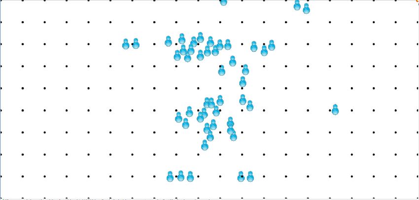
0                                4                                5
                                            0                              0                                  0
                                                                                                                         2
                                                                                                                                              0

                                    0                             1                                                              1
                                                                                                          1
                 0                                3                                4
                                                                                                                     3
                                                                                                                                          1

                             0                            2                                3
                                        0                             2                               2                      2

Fig. 2. A spatial gradient in a simple network in which the nodes are at distance 1 from their neighbours. The grey node is the source, and nodes are labelled
with the known distance from the source. From left: (i) the initial status of the network; (ii) the network once the gradient stabilised (iii) the re-shaping of
the gradient due to a node movement and subsequent link breaking; (iv) the re-shaping of the gradient due to node movement and subsequent new link creation

[12]. For the sake of reproducibility, in Listing 1 we show the                   time@POI() = i f { s . r v a l (13) == 30.0} t h e n s . r v a l (0)             1
                                                                                                                               e l s e #time@POI() f i ;           2
code snippet used to model the scenario in A LCHEMIST.                            e v a l E[ time@POI() ] ;                                                        3

                             III.   M ULTI V E S TA                               Listing 2.   The simple M ULTI Q UATE X expression Q1
                         2
    M ULTI V E S TA is a recently proposed statistical analyzer
for probabilistic systems [11], extending V E S TA [31] and
PV E S TA [32]. The analysis algorithms of M ULTI V E S TA are                    eval clauses. Each eval clause relies on the defined temporal
independent of the used model specification language: it is                       operators, and specifies a system property whose expected
only assumed that discrete event simulations can be performed                     value must be evaluated. As an example, Listing 2 depicts
on the input model. As described in [11], the tool offers a                       the simple M ULTI Q UATE X expression Q1 which intuitively
clean interface to integrate existing discrete event simulators,                  reads as: “compute the expected value of the time necessary to
enriching them with a property specification language, and with                   let all the individuals reach their target”. More in particular,
efficient distributed statistical analysis capabilities.                          lines 1-2 define a recursive temporal operator, composed by
                                                                                  the name of the operator (time@POI()), and by a path
    M ULTI V E S TA performs a statistical (Monte Carlo based)                    expression representing its body, i.e. a real-typed predicate
evaluation of M ULTI Q UATE X expressions, allowing to query                      possibly evaluated after performing steps of simulation. Line
about expected values of observations performed on simulations                    3 provides one eval clause, specifying that we are interested
of probabilistic models. A M ULTI Q UATE X expression may                         in evaluating the expected value of time@POI().
regard more than a measure of a model, in which case the
same simulations are reused to estimate them, thus improving                          In order to evaluate a M ULTI Q UATE X expression, M ULTI -
the performance of the analysis tasks. Moreover, the tool has a                   V E S TA performs several simulations, obtaining from each a list
client-server architecture allowing to distribute the simulations                 of samples (real numbers). One sample for each eval clause is
on different machines. A detailed description of M ULTI Q UA -                    obtained, thus all the queried measures are evaluated using the
TE X and of the procedure to estimate its expressions, omitted                    same simulations, improving performance. When evaluating the
in this work due to space constraints, is given in [11], [33].                    samples of a simulation, s is associated to the initial state of
The tool also supports the transient fragment of probabilistic                    the system, and then the eval clauses are evaluated. Consider
computation tree logic (PCTL) [34] and continuous stochastic                      the simple case of Q1 , having just one eval clause: at the
logic (CSL) [35], [36], for which statistical model checking                      first step of the simulation the guard of the if statement
algorithms based on the invocation of a series of inter-dependent                 (s.rval(13) == 30) is evaluated: “does in s all the 30
statistical hypothesis testing are implemented [37]. However,                     individuals have reached their target?”. If the guard is evaluated
this work focuses on M ULTI Q UATE X, as it generalizes the two                   to true, then s.rval(0) is returned, i.e. the current simulated
mentioned logics [33].                                                            time. Otherwise the expression is evaluated as #time@POI():
                                                                                  M ULTI V E S TA orders the simulator to advance of one step,
    Before defining a M ULTI Q UATE X expression, it is nec-
                                                                                  updates s, and then recursively evaluates time@POI(). Note
essary to specify the state characteristics to be observed.
                                                                                  that the operator # (named next) triggers the execution of a step
This model-specific step “connects” M ULTI Q UATE X with the
                                                                                  of simulation, thus if it is used in recursive temporal operators
simulated model. In particular, the state observations are offered
                                                                                  (like in Q1 ), it allows to query properties of states obtained
via the rval(i) predicate which returns a number in the real
                                                                                  after an unspecified number of steps. The evaluation evolves as
domain for each observation i. As sketched in Section IV,
                                                                                  described until a state satisfying the guard of the if statement
for the crowd steering scenario s.rval(0) corresponds to
                                                                                  is reached (which always happens in the considered model).
the current simulated time, s.rval(3) counts the number of
LSAs in the system, while s.rval(11), s.rval(12) and                                  The case of expressions with more eval clauses is similar,
s.rval(13) count, respectively, the number of people that                         the only difference is that, at each step of the simulation, all the
have reached the POI on the right, the one on the left, and                       eval clauses are evaluated: for each of them, either a real value,
both. Finally, s.rval(14) returns the average connectivity                        or the # operator followed by a temporal operator is returned.
degree of the devices (i.e. sensors and smartphones).                             In the first case, the sample relative to the eval clause is
    A M ULTI Q UATE X expression consists of a set of definitions                 obtained, and thus the eval clause is ignored for the rest of the
of parametric recursive temporal operators, followed by a list of                 simulation, in the second case a step of simulation is required.
                                                                                  The evaluation of the samples in a simulation terminates when
  2 http://code.google.com/p/multivesta/.                                         all the eval clauses completed their evaluation.
1 people@POI(x) = i f { s . r v a l (0) >= x} t h e n s . r v a l (13) people@POI(x) = i f { s . r v a l (0) >= x} t h e n s . r v a l (13) 1
2 e l s e #people@POI(x) f i ; e l s e #people@POI(x) fi; 2
3 e v a l E[ people@POI(30.0) ] ; e v a l E[ people@POI(10.0) ] ; e v a l E[ people@POI(15.0) ] ; 3
e v a l E[ people@POI(20.0) ] ; e v a l E[ people@POI(25.0) ] ; 4
Listing 3. The M ULTI Q UATE X expression Q2 e v a l E[ people@POI(30.0) ] ; e v a l E[ people@POI(35.0) ] ; 5
Listing 5. The M ULTI Q UATE X expression M Q2
Basing on the samples obtained from simulations, M UL -
TI V E S TAestimates the expected values of M ULTI Q UATE X people@POI(x) = i f { s . r v a l (0) >= x} t h e n s . r v a l (13) 1
e l s e #people@POI(x) f i ; 2
expressions with respect to two user-defined parameters: α e v a l p a r a m e t r i c (E[ people@POI(x) ],x,10.0,5.0,35.0) ; 3
and δ. Considering the case of simple expressions with just
one eval clause, the estimations are computed as the mean Listing 6. M Q2 as a parametric multi-expression
value of the n samples obtained from n simulations, with n
large enough to grant that the size of the (1 − α) ∗ 100%
Confidence Interval (CI) is bounded by δ. In other words, if difficult to see that M Q1−2 corresponds to Q1 and Q2 .
a simple M ULTI Q UATE X expression is estimated as x, then,
with probability (1 − α), its actual expected value belongs to Listing 5 provides another interesting multi-expression
the interval [x − δ/2, x + δ/2]. (M Q2 ), that estimates the excepted number of people reaching
their target at the varying of the simulated time (i.e. at time 10,
Again, the case of expressions with multiple eval clauses 15, 20, 25, 30 and 35). In order to ease the writing of multi-
is similar. Note that the eval clauses may regard values of expressions like M Q2 , M ULTI Q UATE X provides parametric
different orders of magnitude, and thus the user may provide a multi-expression (or parametric expression in short), i.e. some
list of δ rather than just one. After having obtained a sample syntactic sugar (a macro) that allows to concisely write multi-
for every eval clause from a simulation, these values are used expressions evaluated at the varying of a parameter. Listing 6
to update the means of the samples obtained from previous depicts a parametric expression corresponding to M Q2 . In
simulations (one mean per eval clause). If the CIs have been line 3, the keyword parametric is used: provided a path
reached for every eval clause, the evaluation of the expression expression (people@POI(x)), a variable (x) and a range
is terminated, otherwise further simulations are performed. of values specified as min (10.0), increment (5.0) and max
Note that each eval clause may require a different number (35.0), the keyword is unrolled in the corresponding list of
of simulations to reach the required CI. Once the CI of an eval clauses (in this case those of Listing 5). Noteworthy,
eval clause has been reached, such eval clause is ignored in parametric takes as first parameter a list of path expressions,
eventual further simulations performed for other eval clauses. allowing to study more measures at the varying of a parameter.
Another interesting expression is Q2 of Listing 3, reading: It is assumed that expressions are properly typed: the guards
compute the expected number of people reaching the target after of if statements must be booleans, while the path expressions
30 units of simulated time. Q2 shows that temporal operators in the eval clauses must be real. Moreover, we restrict to
can have parameters (variables). Variables have to be bounded, bounded expressions, i.e. the subset of expressions which can
i.e. if they are in the right-hand-side of a temporal operator be evaluated performing a finite number of steps of simulation.
definition (i.e. after the equals sign), then they also have to
be in its left-hand-side, so that a value can be assigned to
them. Noteworthy, if rval(13) would evaluate to 1.0 in case IV. I NTEGRATING M ULTI V E S TA AND A LCHEMIST
a certain event happens in a simulation, and to 0.0 otherwise,
then Q2 would estimate the probability of such event. This section describes the integration of M ULTI V E S TA and
A LCHEMIST. Some steps (Section IV-A), have been tackled
The simple expressions Q1 and Q2 query a measure of the once and for all, while others are model-specific, and are thus
system (i.e. rval(0) in Q1 , or rval(13) in Q2 ), while related to the crowd steering scenario (Section IV-B).
one may be interested in more. As said, M ULTI Q UATE X
expressions may have lists of eval clauses, each studying a
different measure. We refer to expressions having more eval A. Simulator-specific integration
clauses as multi-expressions. Intuitively, a multi-expression Essentially, in order to allow the interaction with M UL -
with n eval clauses corresponds to n expressions sharing the TI V E S TA,A LCHEMIST has to fulfill two requirements: (1)
same temporal operators but having each one of the eval the ability to advance the simulation in a step-by-step man-
clauses. However, the multi-expression is more compact and ner (which is provided by the playSingleStepAndWait
is evaluated performing less simulations: just the maximal method in ISimulation interface); (2) the ability to
number of simulations required by the single simple expressions. analyse the model status after each simulation step, providing
Listing 4 provides the multi-expression M Q1−2 . It is not measures in form of real numbers about properties of interest.
Since both M ULTI V E S TA and A LCHEMIST are Java-
1 time@POI() = i f { s . r v a l (13) == 30.0} t h e n s . r v a l (0) based, their interaction has been easily realized by subclass-
2 e l s e #time@POI() f i ;
3 people@POI(x) = i f { s . r v a l (0) >= x} t h e n s . r v a l (13)
ing the NewState class of M ULTI V E S TA. The obtained
4 e l s e #people@POI(x) f i ; AlchemistState class is sketched in Listing 7, where
5 e v a l E[ time@POI() ] ; e v a l E[ people@POI(30.0) ] ; unnecessary details are omitted. The new class contains some
Listing 4. The M ULTI Q UATE X expression M Q1−2 A LCHEMIST-specific code, providing M ULTI V E S TA with the
simulation control and proper entry points for the analysis.1 p u b l i c c l a s s AlchemistState e x t e n d s NewState { ISimulation sim) {
2 p r i v a t e f i n a l EnvironmentBuilder eb; f i n a l IEnvironment env = sim.getEnvironment(); 2
3 p r i v a t e f i n a l l o n g maxS; i n t count = 0; 3
4 p r i v a t e f i n a l ITime maxT; s w i t c h (prop) { 4
5 p r i v a t e ISimulation sim; c a s e PEOPLE_RIGHT: 5
6 ... f o r ( f i n a l INode node : env) { 6
7 p u b l i c AlchemistState( f i n a l ParametersForState params) i f (isInRightArea(node, env)) { 7
throws ...{ count++; 8
8 s u p e r (params); } 9
9 f i n a l StringTokenizer otherparams = new StringTokenizer( } 10
params.getOtherParameters()); r e t u r n count; 11
10 // Initialization of Alchemist-specific parameters and ... 12
execution environment resorting to otherParams c a s e CONNECTIVITY: 13
11 } f o r ( f i n a l INode n : env) { 14
12 ... count+=env.getNeighborhood(n).getNeighbors().size(); 15
13 p u b l i c v o i d setSimulatorForNewSimulation( f i n a l i n t seed) { } 16
14 /* Stop current simulation, create a new one. */ r e t u r n (( d o u b l e ) count) / env.getNodesNumber(); 17
15 ... ... 18
16 sim.stop(); default: 19
17 sim.waitForCompletion(); r e t u r n 0; 20
18 ... } 21
19 env = getFreshEnvironment(seed); } 22
20 sim = new Simulation(env, maxS, maxT);
21 ... Listing 8. AlchemistStateEvaluator for the crowd steering model
22 }
23 ...
24 p u b l i c v o i d performOneStepOfSimulation() {
25 sim.playSingleStepAndWait();
26 } own observations of interest. These are managed resorting to
27 ... the default branch (lines 36-37), as described in Section IV-B.
28 p u b l i c d o u b l e rval( f i n a l i n t obs) {
29 i f (obs >= 0 && obs < StandardProperty.RESERVED_IDS) { The resulting integrated tool has been packaged within
30 s w i t c h (StandardProperty.fromInt(obs)) {
31 c a s e TIME: the standard A LCHEMIST distribution. Simply by downloading
32 r e t u r n getTime(); A LCHEMIST version 4 or newer, the user is enabled to exploit
33 c a s e STEP: the analysis capabilities of M ULTI V E S TA.
34 r e t u r n sim.getStep();
35 ...
36 default: B. Model-specific integration
37 r e t u r n getStateEvaluator().getVal(obs, t h i s );
38 }
39 }
Depending on the model at hand, it may be necessary
40 ... to refine the model-independent observations exposed by
41 } AlchemistState with a set of model-specific ones. This
42 }
can be done by simply instantiating the IStateEvaluator
Listing 7. AlchemistState extending M ULTI V E S TA’s NewState class interface provided by M ULTI V E S TA, constituted by the method
getVal(int observation, NewState state).
Listing 8 sketches AlchemistStateEvaluator, de-
In the constructor (lines 7-11), the superclass initialization fined for the crowd steering scenario. For the sake of brevity,
is done by a simple super() call. The remaining code ini- only two among all the properties of interest are reported: the
tializes A LCHEMIST specific parameters such as the maximum number of people that have reached the POI on the right side
time or number of steps to simulate. It is worth noting that those and the average connectivity of the devices.
are in general not required, since M ULTI V E S TA is generally
able to detect when the analysis requirements has been met, V. A NALYSIS OF THE SCENARIO
and consequently stop the simulation flow.
This section discusses the analysis performed on our crowd
The setSimulatorForNewSimulation() method is
steering scenario, resorting to the integration of M ULTI V E S TA
depitcted in lines 13-22. The goal of the method, invoked
and A LCHEMIST. The outcome of the analysis is summarized
by M ULTI V E S TA before performing a new simulation, is
in the three charts of Figure 3, showing, at the varying of the
to (re)initialize the status of the simulator, generating a new
simulated time, the expected values of: the number of people
simulation with the specified seed.
which have reached their POI (top), the average number of
In lines 24-26, performOneStepOfSimulation() connections of the devices (middle), and the number of LSAs
is provided: resorting to the A LCHEMIST method in the system (bottom).
playSingleStepAndWait(), it allows M ULTI V E S TA to
The three charts have been obtained by evaluating
order the execution of a single simulation step.
M ainM Q of Listing 9, having 5 parametric temporal operators
In order to inspect and analyse the simulation state, the (lines 1-10). people@RPOI and people@LPOI regard the
rval() method defined in lines 28-41 is invoked. The number of people which have reached, respectively, the POI
argument specifies the observation of interest. This method on the right and the one on the left. people@POI counts
inspects the simulation state for all aspects common to any instead how many people have reached their destination. The
A LCHEMIST model, e.g. in Listing 7 lines 31-35 are sketched fourth temporal operator (avgConn) regards the connectivity
the current simulated time and the number of performed degree of the devices. Finally, LSAs regards the number of
simulation steps. Clearly, each A LCHEMIST model will have its LSA in the system. The temporal operators are analysed at thePeople on their target zone people@POI(x) = i f { s . r v a l (0) >= x} t h e n s . r v a l (13) 1
30 e l s e #people@POI(x) f i ; 2
people@RPOI(x) = i f { s . r v a l (0) >= x} t h e n s . r v a l (11) 3
E[People at their destination]
25 Right to left e l s e #people@RPOI(x) f i ; 4
Left to right people@LPOI(x) = i f { s . r v a l (0) >= x} t h e n s . r v a l (12) 5
Total e l s e #people@LPOI(x) f i ; 6
20
avgConn(x) = i f { s . r v a l (0) >= x} t h e n s . r v a l (14) 7
e l s e #avgConn(x) f i ; 8
15 LSAs(x) = i f { s . r v a l (0) >= x} t h e n s . r v a l (3) 9
e l s e #LSAs(x) f i ; 10
10 e v a l p a r a m e t r i c (E[people@POI(x)],E[people@RPOI(x)], 11
E[people@LPOI(x)],E[avgConn(x)],E[LSAs(x)],
5 x,0.0,1.0,50.0);
0 Listing 9. The evaluated parametric multi-expression (M ainM Q)
0 5 10 15 20 25 30 35
Time (simulated seconds)
Average connectivity values, thus indicating the intervals in which the actual expected
11 values lie with probability 0.99.
10.8
E[node connectivity]
A. Comments on the obtained results
10.6
10.4
The top chart regards the first 3 temporal operators: the
top plot refers to the number of people in total which have
10.2 reached their target POI, while the two almost over-imposed
10
lower plots regard the number of people at the right POI and
at the left POI. All the three measures under analysis produced
9.8 monotonically increasing sigmoid curves. We can deduce from
0 5 10 15 20 25 30 35
this behaviour that there are no systemic errors in the crowd
Time (simulated seconds) steering system, such as people with no or wrong suggested
LSAs in the system
final destination, in which case we would have noticed one or
more flatted zones flawing the sigmoid curve. We note also
E[Total number of LSAs in the network]
700
that after around 30 simulated seconds all the people have
600 reached their target, and that it takes around 10 seconds for the
500 fastest walkers to get to their destination. Note that, despite
400
the analysis has been performed for 50 simulated seconds, the
charts presented in Figure 3 have been cut at time 35 to better
300 show the most relevant results: in fact, the system reaches
200 stability after this time, and no event of interest happens later.
100
Moreover we can also notice that people going from left to
right are slightly faster than the other group. This difference,
0
0 5 10 15 20 25 30 35
due to the asymmetric positioning of people in the centre of
Time (simulated seconds)
the scenario, is hardly visible and would have been impossible
to spot with a lower precision analysis.
Fig. 3. Analysis of the crowd steering scenario: (top) number of people at the The middle chart shows the evolution with time of the
POIs, (middle) average number of connections per device, (bottom) number
of LSAs in the system.
average number of connections of the devices (i.e. both sensors
and smartphones). Since each device is considered to be
connected to all those within a range of 1.5 meters, it also
gives us a hint about the crowding level. There is a noticeable
varying of the simulated time from 0 to 50 seconds, with step peak at around 8 seconds: it is due to a high number of people
1 (line 11). Thus the analysis consisted in the estimation of approaching the central group. After that, the peak disappears
the expected values of the 5 temporal operators instantiated when most people overtook the obstacle and are walking
with 50 parameters, for a total of 250 expected values. towards their POI. Finally, there is a growth: progressively,
people reach their destination and tend to create a crowd.
A high degree of precision has been required: α has been
set to 0.01, while the δ values (the size of the CIs) have been The bottom chart shows the number of LSAs in the whole
chosen considering the orders of magnitude of the measures: 0.5 system, indirectly giving hints on the global memory usage.
for the instances of people@POI(x), people@RPOI(x) Once the system is started, there is a very quick growth, due
and people@LPOI(x); 0.05 for avgConn(x); and 3 for to the gradient being spread from the sources to the whole
LSAs(x). To reach such a level of confidence, the tool ran sensors network and to the LSAs produced by the crowd-
approximately 2500 simulations, requiring less than a hour. sensing. The system reaches a substantial stability after a couple
of seconds. From that point on, the number of LSAs has very
The discussed confidence intervals are depicted in the little variations: the system has no “memory leak”, in the sense
aforementioned charts: the two lines drawn above and below that it does not keep on producing new LSAs without properly
the central lines represent the obtained CIs of the expected removing old data.Expressions Parametric expressions Parametric multi-expression
Performance scaling people@POI 39999.32 2567.26 n.a.
Total time / simulations number (seconds)
60000 22.5 people@RPOI 15891.13 1114.86 n.a.
55000 people@LPOI 15560.83 950.30 n.a.
Total execution time (seconds)
20 avgConn 90111.29 1372.64 n.a.
50000
Total execution time 17.5 LSAs 58630.45 2504.33 n.a.
45000
Total time / simulations number Total time 220193.02 8509.39 3215.95
40000 15
35000 12.5
30000 Fig. 5. Time performance improvements reusing simulations (seconds).
25000 10
20000 7.5
15000 5
10000 of Listing 9, analysed in this section, is an example of
5000 2.5 parametric multi-expression. As explicitated by Figure 5 (whose
0 0 reported analysis have been performed resorting to 48 servers),
5 10 15 20 25 30 35 40 45
the parametric expressions (second column) allowed us to save
Number of servers
a stunning 96% of execution time wrt the simple expressions
case without reuse of simulations (first column). Moreover, the
Fig. 4. Performance scaling with of the number of running servers. parametric multi-expression feature (third column) allowed us
to further cut down this time to a third. We can thus advocate
that, by exploiting the feature of reuse of simulations, for the
B. Performance assessment scenario under investigation we obtained a more than 68 times
faster analysis.
All our experiments have been run on an a machine equipped
with four Intel® Xeon® E7540 and 64GB of RAM, running
Linux 2.6.32 and Java 1.7.0 04-b20 64bit. VI. C ONCLUSIONS AND FUTURE WORKS
In order to measure the performance scaling of the tool, This paper presented a novel statistical analysis tool tailored
we ran our analysis multiple times varying the number of to chemical-inspired pervasive systems. The tool has been
M ULTI V E S TA servers deployed. Results are summarized by obtained by combining A LCHEMIST, an efficient state-of-the-
the dark line of Figure 4, showing that with only 1 server, the art simulator for chemical-oriented computational systems, with
analysis required almost 17 hours, while with more than 30 M ULTI V E S TA, a recently proposed lightweight tool which
servers it required less than a hour. For the considered scenario, allows to enrich existing discrete event simulators with efficient
by distributing simulations we have thus obtained a more than distributed statistical analysis capabilities.
18 times faster analysis.
By integrating A LCHEMIST with M ULTI V E S TA, the former
It is worth to note that such comparison of performance has been enriched with capabilities far from those usually
is affected by the statistical nature of the analysis procedure. offered by simulation tools. Mainly, it is now possible to
Indeed, M ULTI V E S TA may need to run a sightly different define in a clean and compact way the properties of interest,
number of simulations in order to obtain the same precision to decouple them from the model definition, and to automatize
in different evaluations. Intuitively, when evaluating a M ULTI - their evaluation. The analysis tasks can be performed efficiently,
Q UATE X expression resorting to x or to x + y servers, in both as the distribution of simulations is supported. Furthermore,
cases we initialize the first x servers with the same x seeds, another important benefit is the ability of evaluating more
generating thus the same x simulations. However, the remaining properties at once via parametric multi-expressions, thus
y servers are initialized with new seeds, and thus produce reducing the number of required simulations and speeding
new simulations. Clearly, by having different simulations, we up greatly the analysis operations.
may obtain different sample variances, requiring a different
number of simulations. For this reason, the bright line of The analysis capabilities and performance of the newly
Figure 4 depicts the time analysis normalized wrt the number of obtained tool have been evaluated in a crowd steering scenario
simulations (obtained dividing the overall analysis time by the regarding 45 smartphone-equipped people moving to a POI,
number of performed simulations). The two lines of Figure 4 immersed in an environment with a grid of 200 computationally
evolve accordingly, thus confirming the great performance gain enabled sensors. The analysis consisted in the estimation, with
brought by the distribution of simulations. high degree of precision, of 250 expected values, and required
less than an hour in total.
As discussed in Section III, other than distribution of
simulations, M ULTI V E S TA has a further important feature M ULTI V E S TA already supports several simulators (as
which dramatically reduces the time necessary to perform discussed in [11]). From now on M ULTI V E S TA is also part
analysis tasks: the tool is able to reuse the same simulations to of the A LCHEMIST distribution, and will be used in future for
estimate many expected values. The reusage happens on two performing analysis on complex scenarios, giving to all the
levels: (1) expressions can be made parametric, and thus the A LCHEMIST users the benefits described in this paper.
same simulations can be used for computing the same property
at the varying of a parameter (e.g. at different time steps). An
example is M Q2 of Listing 6; (2) it is possible to write multi- ACKNOWLEDGMENT
expressions (e.g. M Q1−2 of Listing 4), and thus use the same
simulations to obtain the expected values of multiple properties. Acknowledgements: Work supported by the European projects FP7-
Moreover, by combining these two features, it is possible to FET 256873 SAPERE, FP7-FET 257414 ASCENS, and FP7-STReP
reuse simulations for multiple parametric properties. M ainM Q 600708 QUANTICOL, and by the Italian PRIN 2010LHT4KM CINA.R EFERENCES [19] A. M. Uhrmacher and C. Priami, “Discrete event systems specification
in systems biology - a discussion of stochastic pi calculus and devs,” in
[1] R. Doursat, “Organically grown architectures: Creating decentralized, Proceedings of the 37th conference on Winter simulation, ser. WSC ’05.
autonomous systems by embryomorphic engineering,” in Organic Winter Simulation Conference, 2005, pp. 317–326. [Online]. Available:
computing. Springer, 2008, pp. 167–199. http://dl.acm.org/citation.cfm?id=1162708.1162767
[2] M. Viroli and M. Casadei, “Biochemical tuple spaces for self-organising [20] R. Ewald, C. Maus, A. Rolfs, and A. M. Uhrmacher, “Discrete
coordination,” Coordination Models and Languages, pp. 143–162, 2009. event modeling and simulation in systems biology,” Journal of
[3] M. Mamei, F. Zambonelli, and L. Leonardi, “Cofields: a physically Simulation, vol. 1, no. 2, pp. 81–96, 2007. [Online]. Available:
inspired approach to motion coordination,” Pervasive Computing, IEEE, http://dx.doi.org/10.1057/palgrave.jos.4250018
vol. 3, no. 2, pp. 52–61, 2004. [21] D. T. Gillespie, “Exact stochastic simulation of coupled chemical
[4] F. Zambonelli, G. Castelli, L. Ferrari, M. Mamei, A. Rosi, G. Di reactions,” The Journal of Physical Chemistry, vol. 81, no. 25, pp.
Marzo, M. Risoldi, A.-E. Tchao, S. Dobson, G. Stevenson, Y. Ye, 2340–2361, December 1977. [Online]. Available: http://dx.doi.org/10.
E. Nardini, A. Omicini, S. Montagna, M. Viroli, A. Ferscha, S. Maschek, 1021/j100540a008
and B. Wally, “Self-aware pervasive service ecosystems,” Procedia [22] M. A. Gibson and J. Bruck, “Efficient exact stochastic simulation of
Computer Science, vol. 7, pp. 197–199, Dec. 2011, proceedings of the chemical systems with many species and many channels,” J. Phys. Chem.
2nd European Future Technologies Conference and Exhibition 2011 A, vol. 104, pp. 1876–1889, 2000.
(FET 11). [Online]. Available: http://www.sciencedirect.com/science/ [23] S. Montagna, D. Pianini, and M. Viroli, “A model for drosophila
article/pii/S1877050911005667 melanogaster development from a single cell to stripe pattern formation,”
[5] S. Mariani and A. Omicini, “Molecules of knowledge: Self-organisation in Proceedings of the 27th Annual ACM Symposium on Applied
in knowledge-intensive environments,” Intelligent Distributed Computing Computing. ACM, 2012, pp. 1406–1412.
VI, pp. 17–22, 2013. [24] S. Bandini, S. Manzoni, and G. Vizzari, “Crowd modeling
[6] A. Molesini, M. Casadei, A. Omicini, and M. Viroli, “Simulation in and simulation: Towards 3d visualization,” in Recent Advances
agent-oriented software engineering: The SODA case study,” Science in Design and Decision Support Systems in Architecture and
of Computer Programming, Aug. 2011, special Issue on Agent- Urban Planning, J. P. Leeuwen and H. J. Timmermans, Eds.
oriented Design methods and Programming Techniques for Distributed Springer Netherlands, 2005, pp. 161–175. [Online]. Available:
Computing in Dynamic and Complex Environments. [Online]. Available: http://link.springer.com/chapter/10.1007/1-4020-2409-6 11
http://www.sciencedirect.com/science/article/pii/S0167642311001778 [25] J. Beal, J. Bachrach, D. Vickery, and M. Tobenkin, “Fast self-healing
[7] E. Babulak and M. Wang, “Discrete event simulation: State of the art,” gradients,” in Proceedings of the 2008 ACM symposium on Applied
iJOE, vol. 4, no. 2, pp. 60–63, 2008. computing. ACM, 2008, pp. 1969–1975.
[8] S. Bandini, S. Manzoni, and G. Vizzari, “Agent based modeling [26] J. Beal, “Flexible self-healing gradients,” in Proceedings of the 2009
and simulation: An informatics perspective,” Journal of Artificial ACM symposium on Applied Computing. ACM, 2009, pp. 1197–1201.
Societies and Social Simulation, vol. 12, p. 4, 2009. [Online]. Available: [27] J. L. Fernandez-Marquez, G. D. M. Serugendo, S. Montagna, M. Viroli,
http://EconPapers.repec.org/RePEc:jas:jasssj:2009-69-1 and J. L. Arcos, “Description and composition of bio-inspired design
[9] C. M. Macal and M. J. North, “Tutorial on agent-based modelling and patterns: a complete overview,” Natural Computing, pp. 1–25, 2013.
simulation,” Journal of Simulation, vol. 4, no. 3, pp. 151–162, 2010. [28] S. Montagna, M. Viroli, M. Risoldi, D. Pianini, and G. Di Marzo
[10] D. Pianini, S. Montagna, and M. Viroli, “Chemical-oriented simulation Serugendo, “Self-organising pervasive ecosystems: a crowd evacuation
of computational systems with Alchemist,” Journal of Simulation, 2013. example,” Software Engineering for Resilient Systems, pp. 115–129,
[Online]. Available: http://www.palgrave-journals.com/jos/journal/vaop/ 2011.
full/jos201227a.html [29] S. Montagna, D. Pianini, and M. Viroli, “Gradient-based self-organisation
[11] S. Sebastio and A. Vandin, “MultiVeStA: Statistical Model Checking patterns of anticipative adaptation,” in Self-Adaptive and Self-Organizing
for Discrete Event Simulators,” submitted to ValueTools 2013. Systems (SASO), 2012 IEEE Sixth International Conference on. IEEE,
2012, pp. 169–174.
[12] M. Viroli, D. Pianini, S. Montagna, and G. Stevenson, “Pervasive
[30] M. Chraibi, M. Freialdenhoven, A. Schadschneider, and A. Seyfried,
ecosystems: a coordination model based on semantic chemistry,” in
“Modeling the desired direction in a force-based model for pedestrian
27th Annual ACM Symposium on Applied Computing (SAC 2012),
dynamics,” arXiv preprint arXiv:1207.1189, 2012.
S. Ossowski, P. Lecca, C.-C. Hung, and J. Hong, Eds. Riva del
Garda, TN, Italy: ACM, 26–30 Mar. 2012. [Online]. Available: [31] K. Sen, M. Viswanathan, and G. Agha, “Vesta: A statistical model-
http://dl.acm.org/citation.cfm?doid=2245276.2245336 checker and analyzer for probabilistic systems,” in Quantitative Evalua-
tion of Systems, 2005. Second International Conference on the, 2005,
[13] M. Schumacher, L. Grangier, and R. Jurca, “Governing environments pp. 251–252.
for agent-based traffic simulations,” in Proceedings of the 5th
international Central and Eastern European conference on Multi- [32] M. AlTurki and J. Meseguer, “Pvesta: A parallel statistical model
Agent Systems and Applications V, ser. CEEMAS ’07. Berlin, checking and quantitative analysis tool,” in CALCO, ser. Lecture Notes
Heidelberg: Springer-Verlag, 2007, pp. 163–172. [Online]. Available: in Computer Science, A. Corradini, B. Klin, and C. Cı̂rstea, Eds., vol.
http://dx.doi.org/10.1007/978-3-540-75254-7 17 6859. Springer, 2011, pp. 386–392.
[14] S. Bandini, S. Manzoni, and G. Vizzari, “Crowd Behavior Modeling: [33] G. A. Agha, J. Meseguer, and K. Sen, “PMaude: Rewrite-based
From Cellular Automata to Multi-Agent Systems,” in Multi-Agent specification language for probabilistic object systems,” in QAPL 2005,
Systems: Simulation and Applications, ser. Computational Analysis, ser. ENTCS, A. Cerone and H. Wiklicky, Eds., vol. 153(2). Elsevier,
Synthesis, and Design of Dynamic Systems, A. M. Uhrmacher and 2006, pp. 213–239.
D. Weyns, Eds. CRC Press, Jun. 2009, ch. 13, pp. 389–418. [Online]. [34] H. Hansson and B. Jonsson, “A logic for reasoning about time and
Available: http://crcpress.com/product/isbn/9781420070231 reliability,” Formal Asp. Comput., vol. 6, no. 5, pp. 512–535, 1994.
[15] M. J. North, T. R. Howe, N. T. Collier, and J. R. Vos, “A declarative [35] A. Aziz, V. Singhal, and F. Balarin, “It usually works: The temporal
model assembly infrastructure for verification and validation,” in logic of stochastic systems,” in CAV, ser. Lecture Notes in Computer
Advancing Social Simulation: The First World Congress, S. Takahashi, Science, P. Wolper, Ed., vol. 939. Springer, 1995, pp. 155–165.
D. Sallach, and J. Rouchier, Eds. Springer Japan, 2007, pp. 129–140. [36] C. Baier, J.-P. Katoen, and H. Hermanns, “Approximate symbolic model
[16] E. Sklar, “Netlogo, a multi-agent simulation environment,” Artificial checking of continuous-time markov chains,” in CONCUR, ser. Lecture
Life, vol. 13, no. 3, pp. 303–311, 2007. Notes in Computer Science, J. C. M. Baeten and S. Mauw, Eds., vol.
1664. Springer, 1999, pp. 146–161.
[17] C. Priami, “Stochastic pi-calculus,” Comput. J., vol. 38, no. 7, pp. 578–
589, 1995. [37] K. Sen, M. Viswanathan, and G. Agha, “On statistical model checking
of stochastic systems,” in CAV, ser. Lecture Notes in Computer Science,
[18] T. Murata, “Petri nets: Properties, analysis and applications,” Proceedings K. Etessami and S. K. Rajamani, Eds., vol. 3576. Springer, 2005, pp.
of the IEEE, vol. 77, no. 4, pp. 541–580, Apr. 1989. [Online]. Available: 266–280.
http://dx.doi.org/10.1109/5.24143You can also read