STELLAR SPECTROSCOPY II - DETERMINATION OF STELLAR PARAMETERS AND ABUNDANCES Lezione VII-Fisica delle Galassie

STELLAR SPECTROSCOPY
 II.
DETERMINATION OF STELLAR PARAMETERS
 AND ABUNDANCES

 Lezione VII- Fisica delle Galassie
 Cap 8-9 Carrol & Ostlie

 And
 For neural network in astronomy:
 Leung & Bovy (2018)

 Laura Magrini

OUTLINE of the lecture (continuing from the previous lecture):

The aim of this lecture is to learn how we can obtain information about the
stellar parameters (temperature, surface gravity, global metallicity and
individual element abundances) from a stellar spectrum

 Globally it is a blackbody, but each
 small portion of the spectrum contains a
 large quantity of information

• The conditions for local thermodynamic equilibrium (LTE) are
 satisfied, and so, as already seen, the source function is equal to
 the Planck function, Sλ = Bλ

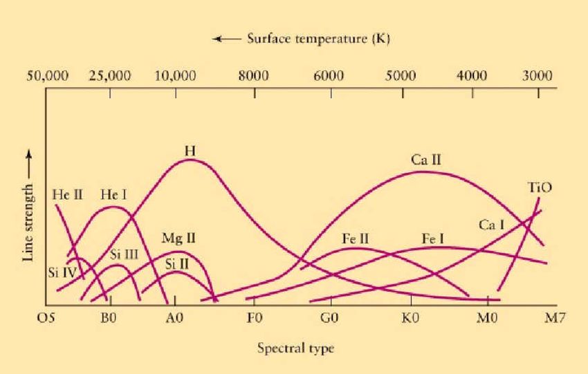
The formation of absorption
 lines
• Absorption lines are created when an atom absorbs a photon with exactly the same
 energy necessary to make an upward transition from a lower to a higher orbital
• The energy of photons depends on the types of stars (their effective Temperature)

What is an equivalent width?
The equivalent width of a spectral line is a
measure of the area of the line on a plot of
intensity versus wavelength.

It is found by forming a rectangle with a
height equal to that of continuum emission,
and finding the width such that the area of
the rectangle is equal to the area in the
spectral line.

It is a measure of the strength of spectral
features.

It is usually measured in mÅ.

What is an equivalent width?
• The opacity κλ of the stellar material is
 greatest at the wavelength at the center
 and it decreases moving into the wings.

• The center of the line is formed at
 lower T, thus in cooler regions of the
 stellar atmosphere.

• Moving into the wings from , the line
 formation occurs at higher T

• It merges with the continuum
 produced at an optical depth of 2/3.

Formation of an absorption line

 Form Lectures of H. Ludwig

• Hot, i.e. bright, continuous spectrum emitted in the deepest layers of the photosphere

• Part of the emitted light is intercepted by absorbing atoms in the higher atmosphere on the
 way out, forming the absorption line

Formation of an absorption line

 Form Lectures of H. Ludwig

• If the number of the absorbers increases, the line becomes deeper, and then it saturates

Line broadening
 Natural broadening:

Due to the uncertainty principle of Heisenberg, an electron in an excited states occupies its orbital for a short time, thus the
energy cannot be precise

 ΔE≃ / Δt (uncertainty in the energy)

Considering that the energy of a photon can be expressed as E=hc/λ , the associate uncertainty is

 2
 Δλ≃ λ /(1/ Δtin + 1/ Δtfin)
 "
where Δtin and Δtfin are the lifetimes of the electron in the initial and final states

• The lifetime of an electron in the first and second excited states of hydrogen is about Δt = 10−8 s.
• The natural broadening of the Hα line of hydrogen, λ = 656. 3 nm, is then Δλ ≈ 4. 57 10−5 nm~ 5 10-4 A~0.5 mA

Line broadening
 Doppler broadening:

In thermal equilibrium, the velocities of atoms (with mass m) follow the Maxwell-Boltzmann
distribution with the most probable velocity

 $%&
 V=√
 '

Since the atoms are moving, the wavelengths of the light absorbed or emitted by the atoms in the gas are
Doppler-shifted according to Δλ/λ = ±|vr |/c .

 Δλ≃ 2λ √
 2 $%&
 " '

The Doppler broadening of the Hα line of hydrogen, λ = 656. 3 nm in the Solar photosphere (T~5777 k),
 is then Δλ ≈ 4. 3 10−2 nm.

à The Doppler broadening is ~1000 greater than the natural broadening

Line broadening
 Pressure broadening:
The orbitals of an atom can be perturbed in a collision with a neutral atom or an ion. The results is called
collisional or pressure broadening.
The general shape of the line is like that found for natural broadening à damping profile or Lorentz
profile
An approximate calculation of the broadening can be done estimating the time between collision:

 ) +
 Δt = =
 * ,- $%&/'

with l mean free path, that can be expressed with , in which n number density and σ collision cross
section

 2
 The corresponding broadening is: Δλ ≃ λ 1/Δt
 C"

 2 $%&
 Δλ≃ λ n √
 C" '

The pressure broadening of the Hα line of hydrogen, λ = 656. 3 nm in the Solar photosphere (T~5777 k),
is then Δλ ≈ 2. 6 10−5 nm, similar to the natural broadening (but it depends in the condition of the star,
it can be much higher)

Line broadening
 Pressure broadening:
The broadening is proportional to the number density: narrower lines observed for the more luminous
giant and supergiant stars are due extended low density atmospheres. The typical pressure broadening
is similar to natural broadening.

Comparison of spectral line widths for A3 I and A3 V class stars. The broader lines for the V luminosity class star arises due
to the denser outer layers in the atmosphere of the main sequence star.

From http://outreach.atnf.csiro.au/education/senior/astrophysics/spectra_astro_types.html.

Line broadening
 Voigt profile:

The combination of Damping and Doppler profiles give a total profile called à Voigt profile

• Doppler broadening dominates near the center

• Damping dominates on the wings of the line

Calculation of spectral lines
• The shape and intensity of a spectral line is related to the abundance of the element Na, but not
 only….

• We need to know, how photons interacts with atoms:

 Ø Temperature and density to solve the Boltzmann and Saha equations (and to determine the
 broadening of the lines)

 Ø The probability of a given transition within the orbitals

 • The relative probabilities of an electron making a transition from the same initial orbital
 are given by the f –values or oscillator strengths for that orbital.

 • For instance: for hydrogen, f= 0. 637 for the Hα transition and f =0. 119 for Hβ.

Our goal is to determine the value of Na by comparing the calculated and observed line profiles.

Digression: how abundances are defined in astrophysics
• Abundances by mass, Z
The proportion of the matter made up of elements heavier than helium (Y) and hydrogen (X).
It is denoted by Z, which represents the sum of all elements heavier than helium, in mass fraction.
 X+Y+Z=1

Solar Z is 0.0134 (Asplund et al. 2009, ARAA 47, 481)

• Abundances by number (gas abundances)
The metallicity of gas is usually expressed by the number ratio of oxygen atoms (or other elements) to hydrogen atoms per
unit volume.
Usually a factor 12 is summed to the final value:
 O/H=log10(NO/NH)+12
 where NO and NH are the numbers of oxygen and hydrogen atoms per unit volume.

• Abundances by number, referred to Solar values (stellar abundances)
The metallicity of stars is usually expressed by the number ratio of iron atoms to hydrogen atoms per unit volume, with
respect to the solar values:
 [Fe/H] = log10(NFe/NH)star - log10(NFe/NH)Sun,
 where NFe and NH are the numbers of iron and hydrogen atoms per unit volume.

Digression: how abundances are defined in astrophysics
• From Z to [Fe/H]

fFe(α) is the number fraction of iron with respect to all the elements heavier than helium; mH is
the mass of the hydrogen atom; and mZ(α) is the average atomic mass of heavy elements weighted
by the number of atoms.

It is important to note that fFe(α) and mZ(α) depend on the fraction of α-elements ([α/Fe]).

• Here a tool online to convert Y and Z in to [Fe/H]:

 http://www2.astro.puc.cl/pgpuc/FeHcalculator2.php

Y~25% by mass, 8% by number of atoms

Going back…from absorption lines to number of absorbers
The curve of growth
The curve of growth is a curve that shows how the equivalent width of an absorption line
increases with the number of atoms producing the line.

The EWs of line depends on the number of absorber atoms [three regimes]

 • When the density of those atoms
 is small, the EWs grows linearly with
 their density (N)

 • When the density become higher the EWs
 tends to saturate, and thus it cannot be used as
 an indication of the abundances of the atoms

 • Finally the EWs is again proportional
 to the abundance (√N)

The curve of growth
• The number of absorbing atoms (abundance) can be determined by comparing the equivalent widths
 from different absorption lines produced by the same atom/ion in the same state (and so having the
 same column density in the stellar atmosphere) with a theoretical curve of growth.

 • On a common
 wavelength
 scale

 • Considering the
 oscillator
 strength of each
 line

The curve of growth
• A curve-of-growth analysis can also be applied to lines originating from atoms or ions in
 different initial states

 1. applying the Boltzmann equation to the relative numbers of atoms in different
 states of excitation allows us to calculate the excitation temperature à in LTE
 approximation it is the effective temperature

 2. It is possible to use the Saha equation to find either the electron pressure or the
 ionization temperature (if the other is known) in the atmosphere from the relative
 numbers of atoms at various stages of ionization.

Determination of stellar parameters from spectral analysis

1. Deriving the EFFECTIVE TEMPERATURE (from Boltzmann equation):

To compute the Teff of a star from its
spectrum, we require that the abundance of
an element is independent of the excitation
potential of the individual lines.

This is so because, all the lines of a given
element should give the same abundance
for the same star.

In practice, there is a (small) scatter around
 To use this method, we need many lines of a single
an average value. element sampling a range of EP, as for example FeI
 lines in cool stars (F-G-K stars).

A Teff which is incorrect will affect the weak
excitation potentials more than the strong
potentials or vice versa.

Determination of stellar parameters from spectral analysis

1. Deriving the EFFECTIVE TEMPERATURE (from Boltzmann equation):

 -500 K

 Lower EP à need more energy to be excited

 correct
 temperature

 If Teff is the correct one, all lines give the same abundance

 +500 K

 Higher EP à need less energy to be excited

Determination of stellar parameters from spectral analysis

2. Deriving the Pressure (proxy of surface gravity) (from Saha equation):

The surface gravity of a star of mass M⋆ and radius R⋆ is defined as g⋆ = GM⋆/R ⋆ 2, where G is the
gravitational constant.

For stellar types F, G or K, we can easily For the hydrostatic equilibrium condition,
measure elements in two ionization states, gravity is related to the gas pressure.
like FeI and FeII.
 From the Saha equation, we found that the
For a given star and a given element, there ratio between FeI and FeII depends on Pe
should be a single value for the abundance, N FeII/N FeI ∝ 1/Pe
no matter if the abundance is determined Assuming that the star is in ionization
from the neutral or the ionized state. equilibrium, we can estimate the pressure, and
 thus the surface gravity
We can then iterate on the gravity of our
model until the abundance of Fe I and Fe II à thus the ionization equilibrium is a good
are the same, constraining the stellar gravity. tool to derive gravity.

Determination of stellar parameters from spectral analysis

2. Deriving the Pressure (proxy of surface gravity) (from Saha equation):

 Mean of the abundance from neutral iron, FeI
 -0.4
 Lines of ionized iron, FeII

 correct
 gravity

 +0.4

The curve of growth for the abundances
Assuming that we derived Teff and log g –from spectroscopic analysis or for photometric analysis-,
we can now use the equivalent widths of different elements/transitions to derive the abundances

For weak lines (first regime) we have:

 transition Absorption
 Equivalent Constant for a given Abu Effective
 coefficient
 nda probability temp
 width of a star nce
 line

 • For weak lines, the equivalent width varies in a linear way with abundances

 • The abundance of an element (A) varies with the inverse of the temperature

 • The abundance depends linearly on the gf -values.

Determination of abundances:
the effect of temperature and gravity
 For instance:

 The strength of lines of ionized elements
 depends on the pressure (log g) and so
 their curve of growth
 depends on the pressure/density
 à log g affects ionized species though Kv

 The dependence on Teff is even stronger

 (from Grey, Lecture on spectral-line
 analysis)

We need to derive Teff and pressure (related to the surface gravity log g) to correctly measure
abundances.

Determination of abundances
Once derived Log g and Teff, from the EWs of absorption lines we can derive the abundances using
their theoretical curve of growth [in which we have fixed Teff and log g] à the comparison gives us
the abundance
 Which elements?

 Depending on the Teff, there are
 different dominating species in the
 atmospheres of stars.

 Limiting the parameter space where
 our approximations are valid

 à Iron I and Iron II dominates and
 allows us both Teff and Log g
 determination

Stellar atmosphere models
 Thus to solve the Boltzmann and Saha’s equations, we must know to the conditions inside the
 stellar atmospheres, specifically:

 • Temperature
 • Pressure (or Log g)
 • Opacity

 The characteristics of the stellar atmospheres are tabulated in several sets of model stellar
 atmospheres, e.g.:

 • Kurucz models: http://kurucz.harvard.edu/grids.html
 • MARCS models: http://marcs.astro.uu.se/
 • ATLAS modes: http://www.stsci.edu/hst/observatory/crds/castelli_kurucz_atlas.html

Stellar atmosphere models
Stellar atmospheric models are a tabulation of
physical parameters used to represent the
conditions inside an atmosphere.

Models are typically given as the electronic
pressure (Pe), the temperature (T) and the
optical depth for photons with λ=5000Å for
several layers (∼50) of a stellar atmosphere.

 • depth in column mass or optical depth at standard
It is customary in stellar atmosphere work to
 wavelength
use log g as equivalent for the pressure in the
 • temperature in K
atmosphere (which can be done if hydrostatic
 • number density of free electrons in cm -3
equilibrium is valid).
 • number density of all other particles (except
 electrons) in cm -3
 • column: density in g/cm 3

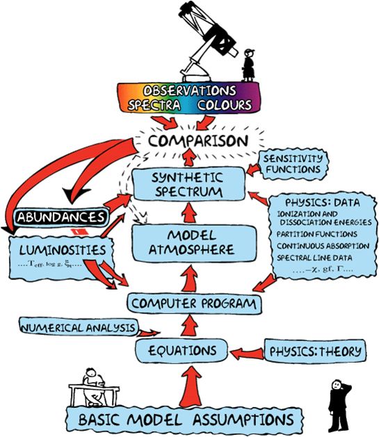
How-to

 Observed spectrum
 EW analysis

 +

 Model Atmosphere

 à
 Stellar parameters and abundances

Boltzmann and Saha’s equations, LTE, pp, etc.

Tools –some examples-
To measure EWs:
§ IRAF splot
§ Daospec http://www.cadc-ccda.hia-iha.nrc-
 cnrc.gc.ca/en/community/STETSON/daospec/
§ Ares http://www.astro.up.pt/~sousasag/ares/

Model Atmospheres:

■ Kurucz models: http://kurucz.harvard.edu/grids.html
■ MARCS models: http://marcs.astro.uu.se/
■ ATLAS modes: http://www.stsci.edu/hst/observatory/crds/castelli_kurucz_atlas.html

ATOMIC DATA:
• VALD: http://vald.astro.uu.se/

• NIST: http://physics.nist.gov/PhysRefData/ASD/lines_form.html

Tools –some examples-

to derive abundances:

§ MOOG http://www.as.utexas.edu/~chris/moog.html
§ ATLAS/SYNTHE (Kurucz) http://kurucz.harvard.edu
• (OS)MARCS: http://marcs.astro.uu.se/
• SME http://tauceD.sfsu.edu/Tutorials.html
§ Synspec http://nova.astro.umd.edu/Synspec43/synspec.html
§ ISPEC: https://www.blancocuaresma.com/s/iSpec
§ THE CANNON: https://www.sdss.org/dr14/irspec/the-cannon

Which elements we can measure:
The main ones are in cool stars:

Alpha-elements: O, Si, Mg, Ca, Ti

Iron-peak elements: V, Sc, Ni, Cr, Fe

Neutron-capture elements: Y, Eu, Ba

Is it enough?
In the previous slides, we have presented the spectral analysis based on several
assumptions, in particular LTE, hydrostatic equilibrium, homogeneity of stellar
atmospheres.

Reality is much more complex:

■ 1D vs 3D results

■ LTE vs NLTE

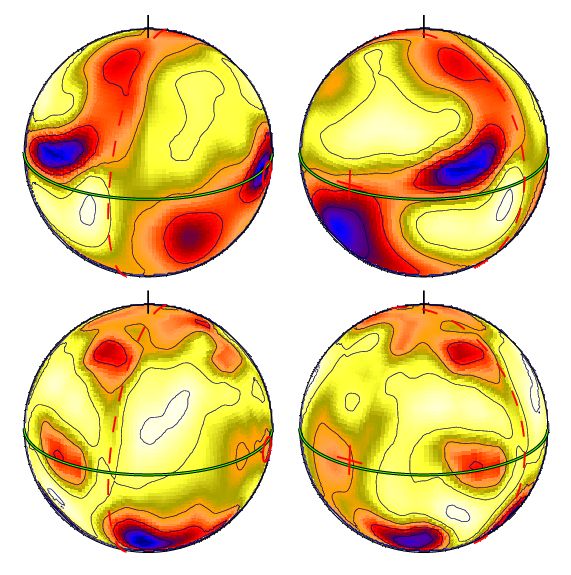
Homogeneity
■ Stellar atmospheres are not homogeneous.

■ They can have sunspots, granulations, non-radial
 pulsations, stellar spots in magnetic stars, clumps
 and shocks in hot star, winds etc.

Stationarityà hydrostatic equilibrium
■ The assumption of stationarity is valid in most
■ Exceptions: pulsating stars, supernovae, mass transfer in close
 binaries, etc.

Conservation of energy
■ Nuclear reactions and production of energy: stellar interiors
■ Negligible production of energy in the stellar atmospheres
■ Energy flux is conserved at any radius

 Local Thermodynamic Equilibrium

■ A star is far to be in thermodynamic equilibrium, since the energy is transported
 from the stellar interior to the surface

■ However in small volumes, we can assume LTE

■ We can consider T(r) as a function of stellar radius

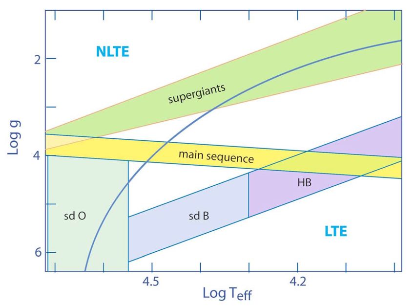
LTE vs. non-LTE
for particular conditions in stellar atmospheres LTE is no more a good approximation….

When we have to take non-LTE into account?
■ Rate of photon absorptions >> rate of collisions

■ Stellar atmospheres characterized by:
q High temperatures
q Low densities

 R. Kudritzki
 lecture

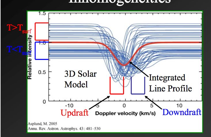
3D vs. 1D
if we want to consider the three-dimensional structure of the photosphere, taking into
account inhomogeneity….
 The stellar photosphere is characterized by:
 • convective flows
 • pulsating waves
 • rotating tornados
 • small-scale turbulent motions.

 The movie above is produced from a 3D computer
 simulation of these processes produced by Uppsala
 astronomers with the CO5BOLD code.

 Just like stationary 1D model atmospheres,
 dynamical 3D models are used to analyse observed
 stellar spectra, allowing in addition to study the
 effects of temperature fluctuations and motions.

 From these comparisons of observed and synthetic
 spectra, not only the properties of the stellar
 atmospheres themselves can be deduced, but also
https://www.physics.uu.se/research/astronomy-and-space-physics/research/stars/model- those of the interior and the outer envelope.
atmospheres/

3D vs. 1D
if we want to consider the three-dimensional structure of the photosphere, taking into
account inhomogeneity….the line profile changes because of the temperature variations

Figure from M. Bergemann

For a review on the effects of 3D and NLTE models:
New Light on Stellar Abundance Analyses: Departures from LTE and Homogeneity
M. Asplund
Annual Review of Astronomy and Astrophysics
Vol. 43:481-530 (September 2005)
https://doi.org/10.1146/annurev.astro.42.053102.134001

Effect of NLTE

 Our understanding of the mechanisms of

 production of some elements are related

 to incorrect abundance measurements

 For instance, manganese:

 • strong non-local thermodynamic

 equilibrium effects

 • but excellent observational databases
Battistini & Bensby (2015)

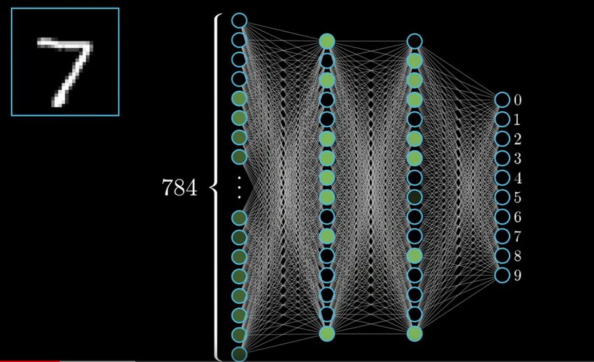
Automactic methods for stellar abundances
Galactic archaeology aims to determine the evolution of the Galaxy from the chemical and kinematical
properties of its individual stars.

This requires the analysis of data from large spectroscopic surveys, with sample sizes in tens of
thousands at present, with millions of stars being reached in the near future.

Such large samples require automated analysis techniques and classification algorithms to obtain
robust estimates of the stellar parameter values (and abundances).

 The sky coverage of three different galactic surveys: APOGEE (in black),
 Gaia-ESO (in red), and GALAH in blue.

Statistical methods for stellar abundances
• Methods based on the measurement of the EWs or on the synthesis of single absorption lines

• The determination of stellar parameters with these methods relies on the Boltzmann and Saha

 equations, and they are valid in the limits of LTE (and other approximations)

Pros:

• Stellar parameters and abundances measured with these methods have a strong physical basis

 (ionization and excitation equilibrium for the stellar parameters, curve of growth for the individual

 abundances)

Cons:

• They work better for high-resolution spectra (to avoid blends between lines, to measure continuum)

• Good knowledge of the atomic physics behind the line formation--> importance of a proper line list

New methods for stellar abundances
Grid of synthetic spectra: e.g. the Ambre project

• Comparison of the observed spectrum with a grid of

 synthetic spectra

• 2 minimization to find the ‘closer’ spectrum

• Determination of the stellar paramters

Pros:

• Full automatic and quick analysis
 AMBRE project:
• Can work also at lower resolution

Cons: designed to automatically analyse the spectral
 archives of the FEROS, UVES, HARPS and
• Degeneracy between temperature, gravity and FLAMES instruments with the MATISSE

 metallicity in some regions of the parameter space algorithm

• Need of a large spectral range (to avoid degeneracy)

New methods for stellar abundances
Grid of synthetic spectra: e.g. the Ambre project

 Using only the short
 spectral range of the
 spectrograph on board of
 the Gaia satellite, in some
 regions of the parameter
 space there is a strong
 degeneracy

 From Kordopatis et al. 2011

New methods for stellar abundances
 Using Gaia information to break the degeneracy (for all methods)
 From C.C. Worley

If unappreciated, degeneracies in stellar parameters can introduce biases and systematic errors in derived
quantities for stars
• Gaia, measuring distance, can help to estimate the absolute luminosity of the stars, and thus their gravity
 à breaking the degeneracy (using the definition of surface gravity GM/R2 and the Stefan-Boltzmann
 equation L∝R2 T4)

New methods for stellar abundances
Data driven methods: The Cannon (Ness et al. 2015)

• The Cannon is a data-driven method to determine stellar parameters and abundances (and more generally,

 stellar labels) for stars in large surveys.

• The Cannon relies on a subset of reference stars in the survey, with known labels. These labels can come from

 high resolution analyses from any wavelength regions and from comparisons with the most up to date stellar

 models.

• The Cannon then uses the reference objects with known labels to build a model that relates stellar labels to

 stellar flux at each wavelength.

• That model is then used to infer the stellar labels for the remaining stars in the survey (Ness et al. 2015).

• The Cannon is named after Annie Jump Cannon, who pioneered producing stellar classifications without

 physical models.

From The Data-Driven Approach to Spectroscopic Analyses, M. Ness

New methods for stellar abundances
Data driven methods: The Cannon (Ness et al. 2015)

Pros:

• Can be used to put together data from different surveys (if there are a good number of stars in both surveys to

 built up a common scale)

• Relates stellar flux to stellar labels (stellar parameters and abundances, but also mass and ages)

• Can be used to transfer label from high-resolution to low-resolution surveys

Cons:

• Need a good reference set (training set)

• Generally, you obtain the same kind of stars you put in the reference set

• The link with physics underlying the formation of stellar spectra is hidden (it is still there…in the training

 set...)

From The Data-Driven Approach to Spectroscopic Analyses, M. Ness

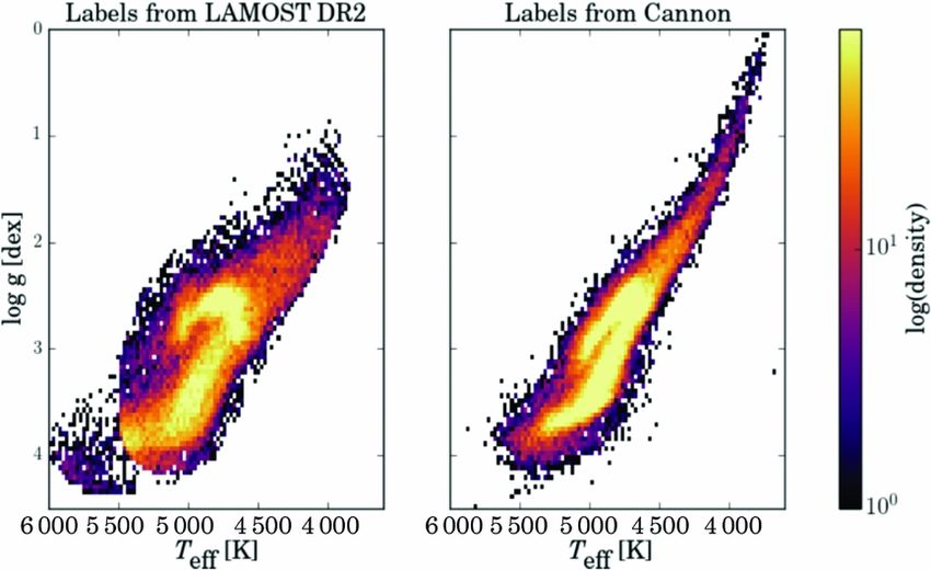
New methods for stellar abundances
Data driven methods: The Cannon (Ness et al. 2015)

à Transferring the information from APOGEE survey (R~28000) to LAMOST (R~2000) with The Cannon

With the Cannon there are plans to put on the same scale (using stars in common):
• 300 000 SEGUE stars
• GALAH (which has currently observed 300 000 stars with the aim to observe 1 million stars)
• APOGEE (which has currently observed 300 000 stars with the aim to observe 450 000 stars)

From The Data-Driven Approach to Spectroscopic Analyses, M. Ness

New methods for stellar abundances
Neural networks: Leung & Bovy (2019) and others (see also Fabbro et al. 2019)

Deep learning using artificial neural networks (ANNs) is getting increasing attention from astronomers, because
of its great potential for data-driven astronomy and its recent successes in many fields such as computer vision,
voice recognition, machine translation, etc.

Progress in ANNs in astronomy:
• Big data (large photometric –SDSS, LSST; astrometric –Gaia; spectroscopic –Gaia-ESO, APOGEE, LAMOST and
 future surveys, …)
• Cheap availability of fast computational hardware (graphics processing units (GPUs) à computer for gaming,
 which are also ideal for ANNs!)
• Advances in the methodology of ANNs
• Availability and accessibility of software platforms implementing this technology (free codes from ANNs, like
 Tensorflow (Abadi et al. 2016), keras (Chollett et al 2015), and astroNN (Leung & Bovy 2019))

The application to high-resolution spectra:
• With a training set of data (~1000 stars) analyzed with more traditional means, ANNs can process high-
 resolution spectra faster and more reliably than other methods

New methods for stellar abundances
Neural networks: Leung & Bovy (2019) and others (see also Fabbro et al. 2019)

There is no need to pre-program any knowledge in an ANN, i.e., neural networks consist of random weights at
the initial training stage.

In order to achieve learning:
• error signals representing the agreement between the true output and the ANN output for (a subset of) the
 training set is back-propagated through the neural network;
• the connection strength of the synapses is adjusted to obtain better agreement between truth and prediction.

 • The ANNs ‘learn’ with the training set
 • The ANNs is then applied to the whole set
 • It can discover features and results that are unexpected

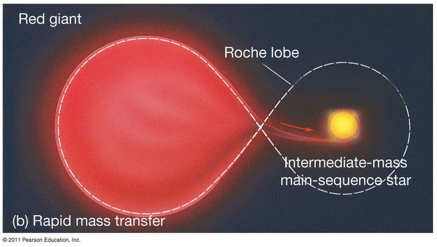
New methods for stellar abundances
Neural networks: Leung & Bovy (2019) and others (see also Fabbro et al. 2019)
• An example, to understand how neural nets work, is how our brain is able to recognize hand-
 written letter and numbers, and associate them with their ‘true’ value
• Similar to the work done by an ANNs to go from high-resolution spectra to low resolution
 spectra

 Matrix to quantify how a hand-written digit can be associated with a number

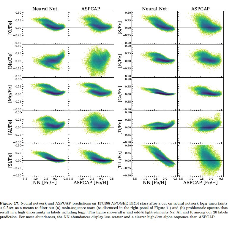
New methods for stellar abundances
Neural networks: Leung & Bovy (2019)

 • ANNs applied to the APOGEE sample

 • Abundance ratios obtained with the neural
 net and with ASPCAP (pipeline of APOGEE
 for the abundances)

 • For most elements the results of the neutral
 net are even tighter than the official results of
 APOGEE

New methods for stellar abundances
 Neural networks and in general data driven methods

 Pros and Cons:

 • They are very similar to the ones of the other data driven methods

 • We need always to start from a well calibrated training set

 • In the training set we must transfer all our knowledge of stellar and atomic physics

à So the physics (of stellar atmospheres) is still there, but is very hidden

à When using the data-driven methods we should not forget which kind of objects we are
 dealing with

Now we know…
 • How to measure stellar parameters from spectral analysis
 • How to use equivalent widths of different elements and transitions to infer their abundance

 ….but
 • We also know that in the standard analysis there are many simplifications (1D, LTE, etc.)
 • New techniques are going towards more sophisticated 3D and NLTE analysis

 ..and
 • For large samples we need to consider other methods
 • Based on good training sets
 • Data driven
 • Fast and automatic

Measuring elemental abundance from stellar spectra is the input for the next step…understanding
the chemical evolution of our Galaxy, acting as Galactic Archeologists.
But first, we want to know where/when/how the different elements are produced.