Stratospheric ozone trends for 1985-2018: sensitivity to recent large variability - atmos-chem-phys ...
←
→
Page content transcription
If your browser does not render page correctly, please read the page content below
Atmos. Chem. Phys., 19, 12731–12748, 2019
https://doi.org/10.5194/acp-19-12731-2019
© Author(s) 2019. This work is distributed under
the Creative Commons Attribution 4.0 License.

Stratospheric ozone trends for 1985–2018:
sensitivity to recent large variability
William T. Ball1,2 , Justin Alsing3,4 , Johannes Staehelin1 , Sean M. Davis5 , Lucien Froidevaux6 , and Thomas Peter1
1 Institutefor Atmospheric and Climate Science, Swiss Federal Institute of Technology Zurich, Universitaetstrasse 16,
CHN, 8092 Zurich, Switzerland
2 Physikalisch-Meteorologisches Observatorium Davos World Radiation Center, Dorfstrasse 33,

7260 Davos Dorf, Switzerland
3 Oskar Klein Centre for Cosmoparticle Physics, Stockholm University, Stockholm 106 91, Sweden
4 Physics Department, Blackett Laboratory, Imperial College London, SW7 2AZ, UK
5 NOAA Earth System Research Laboratory Chemical Sciences Division, Boulder, CO, USA
6 Jet Propulsion Laboratory, California Institute of Technology, Pasadena, CA, USA

Correspondence: William T. Ball (william.ball@env.ethz.ch)

Received: 14 March 2019 – Discussion started: 22 March 2019
Revised: 21 August 2019 – Accepted: 9 September 2019 – Published: 11 October 2019

Abstract. The Montreal Protocol, and its subsequent amend-        a significant overall ozone decrease, with 95 % probability.
ments, has successfully prevented catastrophic losses of          These decreases do not reveal an inefficacy of the Montreal
stratospheric ozone, and signs of recovery are now evident.       Protocol; rather, they suggest that other effects are at work,
Nevertheless, recent work has suggested that ozone in the         mainly dynamical variability on long or short timescales,
lower stratosphere (< 24 km) continued to decline over the        counteracting the positive effects of the Montreal Protocol on
1998–2016 period, offsetting recovery at higher altitudes and     stratospheric ozone recovery. We demonstrate that large in-
preventing a statistically significant increase in quasi-global   terannual midlatitude (30–60◦ ) variations, such as the 2017
(60◦ S–60◦ N) total column ozone. In 2017, a large lower          resurgence, are driven by non-linear quasi-biennial oscilla-
stratospheric ozone resurgence over less than 12 months           tion (QBO) phase-dependent seasonal variability. However,
was estimated (using a chemistry transport model; CTM)            this variability is not represented in current regression analy-
to have offset the long-term decline in the quasi-global in-      ses. To understand if observed lower stratospheric ozone de-
tegrated lower stratospheric ozone column. Here, we ex-           creases are a transient or long-term phenomenon, progress
tend the analysis of space-based ozone observations to De-        needs to be made in accounting for this dynamically driven
cember 2018 using the BASICSG ozone composite. We find            variability.
that the observed 2017 resurgence was only around half
that modelled by the CTM, was of comparable magnitude
to other strong interannual changes in the past, and was
restricted to Southern Hemisphere (SH) midlatitudes (60–          1   Introduction
30◦ S). In the SH midlatitude lower stratosphere, the data
suggest that by the end of 2018 ozone is still likely lower       Ozone in the stratosphere acts as a protective shield against
than in 1998 (probability ∼ 80 %). In contrast, tropical and      ultraviolet radiation that may harm the biosphere, and leads
Northern Hemisphere (NH) ozone continue to display ongo-          to cataracts, skin damage, and skin cancer in humans (Slaper
ing decreases, exceeding 90 % probability. Robust tropical        et al., 1996; WMO, 2014, 2018). In the latter half of the
(> 95 %, 30◦ S–30◦ N) decreases dominate the quasi-global         20th century, the emission of long-lived halogen-containing
integrated decrease (99 % probability); the integrated tropi-     ozone-depleting substances (hODSs) led to approximately a
cal stratospheric column (1–100 hPa, 30◦ S–30◦ N) displays        5 % loss in quasi-global (60◦ S–60◦ N) integrated total col-
                                                                  umn ozone (WMO, 2014), which represents the combined

Published by Copernicus Publications on behalf of the European Geosciences Union.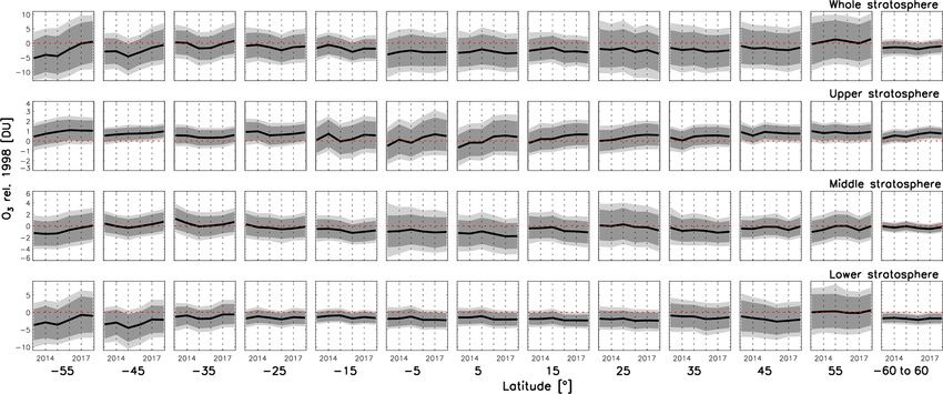
12732                                                                          W. T. Ball et al.: Stratospheric ozone sensitivity

changes in tropospheric and stratospheric ozone contribu-           waves (Hood and Zaff, 1995; Hood et al., 1999) inducing
tions. The 1987 Montreal Protocol and its amendments and            large localised (e.g. over Europe) wintertime decreases in
adjustments led to a reduction in hODSs that resulted in a          ozone. These changes in wave activity might be driven by
halt in total column ozone losses around 1998–2000 (Harris          sea surface temperature and eddy flux changes on decadal
et al., 2015; Chipperfield et al., 2017).                           or longer timescales, although most of these studies are lim-
   However, there is still no evidence of a statistically sig-      ited to the end of the last century when ODSs remained an
nificant increase in total column ozone since 1998 (Chipper-        established primary driver of the decrease. As recent stud-
field et al., 2017; Weber et al., 2018; Ball et al., 2018), de-     ies almost exclusively consider zonal mean ozone fields, this
spite a significant increase in upper stratospheric (1–10 hPa)      motivates the reinvestigation of longitudinal ozone changes
ozone (Ball et al., 2017; Steinbrecht et al., 2017; Ball et al.,    (in future work). The El Niño–Southern Oscillation (ENSO)
2018; Petropavlovskikh et al., 2019). Ball et al. (2018) and        and the quasi-biennial oscillation (QBO) are known to in-
Ziemke et al. (2019) presented evidence, using OMI/MLS              fluence the dynamical variability in the lower stratosphere
tropospheric column observations for 2005–2016, that tro-           and may be main players in driving interannual and decadal
pospheric ozone had also increased significantly. However,          variability in this region (Diallo et al., 2018, 2019). Never-
large uncertainties remain in the quasi-global tropospheric         theless, these dynamical changes do not in themselves de-
ozone trends, and the recent Tropospheric Ozone Assess-             termine a specific underlying driving force; however, the ef-
ment Report (TOAR) shows that different tropospheric ozone          fect of increasing anthropogenic greenhouse gases (GHGs)
products give a wide range of trends, some even indicat-            (Hood and Soukharev, 2005; Peters and Entzian, 1999) on
ing negative changes (Gaudel et al., 2018). The importance          specific mechanisms needs further study (Ball et al., 2018).
of considering tropospheric and stratospheric changes sep-          Conversely, Stone et al. (2018) showed that negative ozone
arately to understand changes in total column ozone has             trends could be simulated in the lower stratosphere over the
also been highlighted in recent studies using chemistry cli-        same period in two of nine ensemble members of a coupled
mate models (CCMs) (Meul et al., 2016; Keeble et al., 2017;         CCM as a result of natural variability interfering in the (lin-
Dhomse et al., 2018). If tropospheric and upper stratospheric       ear) trend analysis, although none of the ensembles displayed
ozone have indeed both increased, then the observed flat            the same widespread negative trends as detected in observa-
trend in total column ozone implies that middle and lower           tions (Ball et al., 2018). They suggested that an additional
stratospheric ozone should have decreased.                          7 years of observations would lead to negative signals disap-
   To assess trends in stratospheric ozone, composites of ob-       pearing in favour of positive trends. The implication, then, is
servations must be formed by merging multiple ozone obser-          that the observed negative trend over the relatively short 19-
vational time series into a long, multi-decadal record from         year timeframe may be a temporary result from large natural
which variability can be attributed, and long-term trends de-       variability (in the single realisation) of the real-world, rather
termined. Composites are subject to artefacts from merg-            than a response to increasing GHGs.
ing different observing platforms. Multiple papers (Tummon             Chipperfield et al. (2018) used a chemistry transport model
et al., 2015; Harris et al., 2015; Steinbrecht et al., 2017; Ball   (CTM) to reconstruct ozone variability close to past real-
et al., 2017, 2018) and a SPARC report (Petropavlovskikh            world behaviour; transport in the CTM is driven by ERA-
et al., 2019) review, discuss, and attempt to account for the       Interim (Dee et al., 2011) reanalysis fields. The results
artefacts in the uncertainty budget.                                showed changes similar to those presented by Ball et al.
   Ball et al. (2018) integrated ozone over the whole strato-       (2018) up to December 2016. They extended their CTM anal-
sphere, i.e. the ozone layer, quasi-globally for pressure lev-      ysis by an additional 12 months to find that the 1998–2016
els from 147–1 hPa (∼ 13–48 km) at midlatitudes (30–60◦ ),          ozone decline in the lower stratosphere (∼ 2 DU; Ball et al.,
and 100–1 hPa (∼ 16–48 km) between the subtropics (30◦ S–           2018) was offset by a sudden increase of ozone in 2017,
30◦ N), and found ozone to be lower in 2016 than in 1998 in         exceeding 8 DU quasi-globally. This was attributed almost
multiple ozone composites. In their analysis, the lower strato-     entirely to dynamical changes and was primarily located in
sphere (147/100–32 hPa, ∼ 13/17–24 km) was driving this             the Southern Hemisphere (SH). Froidevaux et al. (2019) also
decrease. The most significant decreases were in the trop-          noted that ozone trends derived from Aura Microwave Limb
ics, but negative trends extended out into the midlatitudes         Sounder (Aura/MLS) data over a shorter period (2005–2018)
(Fig. 1d). Other studies have subsequently confirmed these          have a tendency towards slightly positive values in the SH,
negative trends (Zerefos et al., 2018; Wargan et al., 2018;         but not so elsewhere within the extra-polar regions. Chip-
Chipperfield et al., 2018). Evidence points towards dynam-          perfield et al. (2018) suggested that the lower stratospheric
ical variations driving changes (Chipperfield et al., 2018),        ozone decrease was a result of large natural variability that
perhaps in the form of enhanced isentropic mixing (Wargan           biased the trend analysis, and that the variability could be
et al., 2018).                                                      attributed to dynamics and not to chemical or photolytic
   Part of the negative trends in northern hemispheric strato-      changes, although the source of dynamical perturbations was
spheric ozone in the 1980s and 1990s at higher latitudes            not identified or the impact on trends quantified. Thus, an as-
have been previously attributed to synoptic and planetary

Atmos. Chem. Phys., 19, 12731–12748, 2019                                           www.atmos-chem-phys.net/19/12731/2019/
W. T. Ball et al.: Stratospheric ozone sensitivity                                                                                  12733

Figure 1. Zonally averaged ozone changes between 1998 and the end years from (a) 2013 to (f) 2018. Red represents increases, and blue
denotes decreases (%; see right-hand legend). Contours represent probability levels of positive or negative changes (see left-hand legend).
Grey shaded regions represent unavailable data. Magenta dashed lines delimit regions integrated to partial ozone columns in other figures.

sessment of this recent variability on trends, and an update to         but we refer to it here as BASICSG . To briefly place the
2018 is needed and is a key aim of this study.                          SWOOSH and GOZCARDS datasets in the context of
   Here, we update the observational analysis of Ball et al.            BASICSG , Fig. S1 of Ball et al. (2018) presented 1998–
(2018) to include data to the end of 2018 (Sect. 3.1). This             2016 changes using SWOOSH or GOZCARDS alone; this
allows us to assess the impact of the 2017 ozone increase in            figure reveals that these ozone composites show generally
the lower stratosphere on the trend analysis, and to consider           similar changes on large spatial scales, although there are
additional changes over 2018. We show that large ozone in-              clear differences on small scales, e.g. in the tropical upper
crease events, with a duration and magnitude similar to that            stratosphere, and in the SH lower stratosphere. Figure S2 of
of 2017 (Chipperfield et al., 2018), have occurred regularly            Ball et al. (2018) importantly demonstrates that there are sig-
since 1985 at midlatitudes (Sect. 3.2), and find that the events        nificant differences between SWOOSH and GOZCARDS at
are linked to a seasonally dependent QBO effect (Sect. 3.3).            100 hPa in the tropical lower stratosphere in the late 1990s;
We update partial column ozone trends from 2016 to 2018 in              this figure also shows that BASICSG is able to account for
Sect. 3.4. Finally, we consider the sensitivity of trends to the        the differences in a principled way that is not simply the av-
recent increase of stratospheric ozone (Sect. 3.5–3.6) by con-          eraging of the two products, which is particularly important
sidering six periods that start in 1985 and end between 2013            for having confidence in an assessment of ozone in the lower
and 2018, in order to demonstrate where signals are robust to           stratosphere. We extend BASICSG from Ball et al. (2018) by
the end date, and where not. Such an analysis is essential to           2 years to cover 1985–2018. This period is essentially an ex-
establish if the negative trends are a result of natural variabil-      tension of the Aura Microwave Limb Sounder (Aura/MLS);
ity interfering in the trend analysis, and to take the first steps      both SWOOSH and GOZCARDS consider Aura/MLS exclu-
to account for what might be driving the large, short-term              sively after 2009.
variability.                                                               We only consider BASICSG here for the following rea-
                                                                        sons. First, as discussed in Ball et al. (2018), compared
                                                                        with the other composites it had the least apparent arte-
2     Data and methods                                                  facts within the time series. The Stratosphere-troposphere
                                                                        Processes And their Role in Climate (SPARC) Long-term
2.1    Ozone data
                                                                        Ozone Trends and Uncertainties in the Stratosphere (LO-
Although other ozone composites exist (Petropavlovskikh                 TUS) report (Petropavlovskikh et al., 2019) indicates this
et al., 2019), we focus exclusively on data formed by merg-             method to be more robust to outliers than other compos-
ing ozone from SWOOSH (Davis et al., 2016) and GOZ-                     ites. Second, BASICSG is resolved in the lower stratosphere,
CARDS (Froidevaux et al., 2015; here we use the v2.20                   which is not the case for all composites. For further discus-
update of Froidevaux et al., 2019) using the so-called BA-              sion see Ball et al. (2018) and the SPARC LOTUS report
SIC (BAyeSian Integrated and Consolidated) approach (Ball               (Petropavlovskikh et al., 2019). Additionally, SWOOSH and
et al., 2017) to account for artefacts in merged composites             GOZCARDS are currently two of the most up-to-date com-
and improve trend estimates. These data were referred to                posites available. Finally, here we are interested in the sen-
as “Merged-SWOOSH/GOZCARDS” by Ball et al. (2018),                      sitivity of stratospheric ozone changes to different end years

www.atmos-chem-phys.net/19/12731/2019/                                                 Atmos. Chem. Phys., 19, 12731–12748, 2019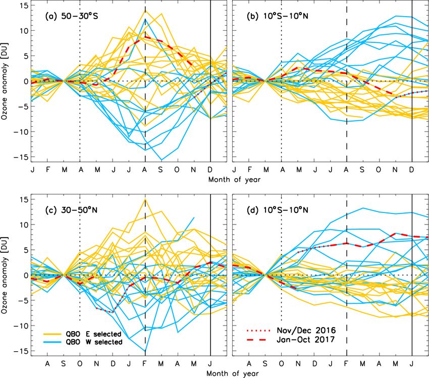
12734                                                                         W. T. Ball et al.: Stratospheric ozone sensitivity

and, as Aura/MLS is arguably one of the best remote-sensing        controlled by a free parameter that is included in the fit (see
platforms for ozone currently in operation (Petropavlovskikh       Supplement, Fig. S1).
et al., 2019), focusing only on BASICSG provides an analy-             Thirdly, in practice MLR is often performed by first sub-
sis, discussion, and interpretation that is free from the com-     tracting an estimated mean seasonal cycle, fitting the trend
plications of considering multiple composites that have mul-       and regressor variables to the anomalies, and then making
tivariate reasons for displaying different behaviour.              a post hoc correction for AR residuals, although many do
                                                                   fit annual and semi-annual components. This procedure typ-
                                                                   ically does not propagate the errors on the seasonal cycle
2.2   Regression analysis
                                                                   and AR parameters in a rigorous way, leading to misrepre-
                                                                   sentation of uncertainties. DLM addresses this by inferring
As in Ball et al. (2018), we perform all time series analyses      all components of the model simultaneously, and formally
using dynamical linear modelling (DLM) (Laine et al., 2014)        marginalising over the uncertainties in all other parameters
utilising the public DLM code DLMMC (available at https://         when reporting uncertainties on, e.g. the trend. We use the
github.com/justinalsing/dlmmc, last access: 9 October 2019).       same prior assumptions as described in Ball et al. (2018).
We provide a short overview of DLM here.                               Probabilities of an overall increase (decrease) in ozone be-
   Our DLM approach models the ozone time series as a              tween two dates (Figs. 1, 7, and Table 1) are computed as the
(dynamical) linear combination of the following compo-             fraction of Markov chain Monte Carlo (MCMC) samples that
nents. There are two seasonal components (with 6- and              show positive (negative) change. Credible intervals (Figs. 6,
12-month periods respectively), a set of regressor variables       8, 9) are computed as the central 95 and 99 percentiles of the
(i.e. proxy time series describing various known drivers), an      MCMC samples. The terms “confidence” and “significance”
auto-regressive (AR) process, and a smooth non-linear (non-        are used interchangeably in this paper with the term “proba-
parametric) background trend. DLM differs from traditional         bility” and specifically refer to Bayesian probabilities; these
multiple linear regression (MLR) approaches in a number of         terms do not refer to the application of frequentist signifi-
key ways.                                                          cance tests and/or confidence intervals.
   Firstly, while MLR fits for a fixed (constant-in-time) linear       We use the same regressors as Ball et al. (2018): solar –
combination of seasonal, regressor, and trend components,          30 cm radio flux, F30 (Dudok de Wit et al., 2014); volcanic
DLM can allow the amplitudes of the various components             – latitudinally resolved stratospheric aerosol optical depth,
to vary dynamically in time, capturing richer phenomenol-          SAOD (Thomason et al., 2018); El Niño–Southern Oscil-
ogy in the data. Here, we allow the amplitude and phase of         lation, ENSO (NCAR, 2013); and the quasi-biennial oscil-
the seasonal components to be dynamic, but keep the regres-        lation, QBO, at 30 and 50 hPa1 . In previous analyses, we
sor amplitudes constant in time. We do this because the sea-       considered the Arctic Oscillation and the Antarctic Oscilla-
sonal cycle in the observational composites can change over        tion, AO/AAO2 , as proxies for Northern Hemisphere (NH)
time, either as a physical feedback of changing temperature        and Southern Hemisphere (SH) surface pressure variability
and ozone or due to different observations exhibiting differ-      only for partial column ozone analysis in their respective
ent seasonal amplitudes (not shown) that are a result of the       hemisphere; here we also consider them for the spatially re-
observing instruments “seeing” slightly different parts of the     solved analysis and use both AO and AAO simultaneously
atmosphere or having different sampling intervals. Due to          in all cases. The AO and AAO have little affect outside their
the seasonal cycle having the largest variability of all modes     respective regions, but we do not limit the possibility that
we expect that, if left unaccounted for, the time varying sea-     they may influence some variability in either hemisphere
sonal modulation might have an influence on the regression.        (Tachibana et al., 2018). We use a first-order AR (AR1) pro-
In principle other regressor amplitudes could also have some       cess (Tiao et al., 1990) to consider autocorrelation in the
time modulation for similar reasons. However, we leave an          residuals. We remove a 3-year period following the Pinatubo
investigation of more flexible DLM models with dynamic re-         eruption, i.e. June 1991 to May 1994, which is 1 year longer
gressor amplitudes to future work where a physically moti-         than the previous analysis, to avoid any effects of the erup-
vated justification for such freedom can be investigated.          tions that may have persisted. Another key point regarding
   Secondly, MLR that does not assume a driver for the long-       the SAOD proxy is that, unlike the other proxies that have
term trends, e.g. for the influence of ODSs or GHGs, typi-         been fully updated to the end of 2018 for this analysis, the
cally assumes a fixed prescription for the shape of the back-      SAOD is currently not extended beyond 2016, so we repeat
ground trend, e.g. a piecewise-linear or independent-linear        the year 2016 for both 2017 and 2018. If any deviations in
trend with some fixed, pre-chosen inflection date. These as-       the SAOD occurred during the 2017–2018 period our analy-
sumptions are both restrictive and give a poor representa-
tion of the smooth background trends we expect from na-               1 QBO   indices: https://www.geo.fu-berlin.de/en/met/ag/strat/
ture (Laine et al., 2014; Ball et al., 2017). DLM addresses        produkte/qbo/index.html (last access: 9 October 2019).
this by instead modelling the trend as a smooth, nonparamet-          2 AO/AAO indices: http://www.cpc.ncep.noaa.gov/products/
ric, non-linear curve, where the “smoothness” of the trend is      precip/CWlink/ (last access: 9 October 2019).

Atmos. Chem. Phys., 19, 12731–12748, 2019                                          www.atmos-chem-phys.net/19/12731/2019/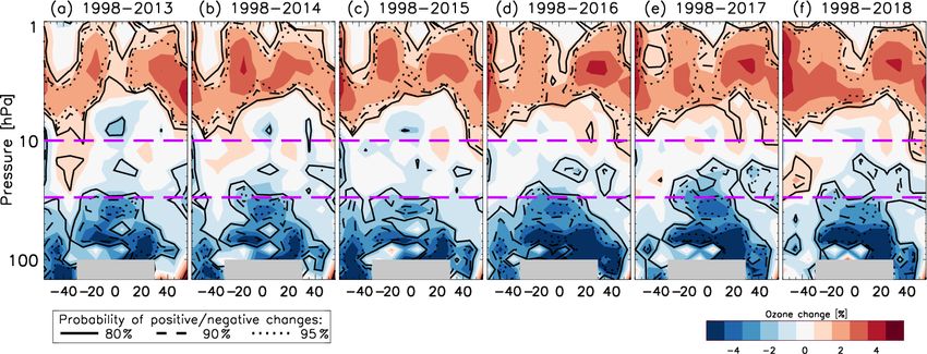
W. T. Ball et al.: Stratospheric ozone sensitivity                                                                           12735

sis will not account for this. Nevertheless, as can be seen in      from negative to positive ozone changes in these regions for
Fig. 1d in this paper, in comparison to Fig. 1b of Ball et al.      any of the 6 end years.
(2018), all of these adjustments to the procedure from Ball            The reduced probability of a SH decrease is related, as we
et al. (2018) have little impact on the estimated mean changes      will see in Sect. 3.2, to the rapid 2017 increase in SH mid-
in ozone.                                                           latitude lower stratospheric ozone reported by Chipperfield
                                                                    et al. (2018) using a CTM. However, Fig. 1 also confirms
                                                                    in observations that this is localised to south of 30◦ S and
3     Results                                                       does not reveal coherent or consistent behaviour over time
                                                                    with the NH, suggesting that there may be large, hemispher-
3.1    Stratospheric ozone changes since 1998                       ically independent variability interfering with the trend esti-
                                                                    mates. Nevertheless, there are currently no signs of an ozone
Figure 1d shows the pressure–latitude, spatially resolved           increase underway in the quasi-global lower stratosphere.
1998–2016 ozone change, reproducing Fig. 1b of Ball et al.             Further, the decrease in ozone in the tropical lower strato-
(2018). Minor differences exist because the BASICSG com-            sphere increases in magnitude and significance as more data
posite and DLM procedure have been updated. Ozone in                are added. The tropical lower stratospheric ozone is pro-
the lower stratosphere (delimited by the pink dashed line at        jected to decrease by the end of the century in all CCMs
32 hPa, or 24 km) shows a marked and almost hemisphere-             (Dhomse et al., 2018), due to enhanced upwelling from the
symmetric decrease, whereas upper stratospheric changes             Brewer–Dobson circulation (BDC) as a result of changes
(> 10 hPa, 32 km) are mainly positive. The middle strato-           to stratospheric dynamics from increasing GHGs (Polvani
sphere generally shows relatively flat ozone trends from 1998       et al., 2018). It is possible that this is a detection in obser-
with low probability of an overall change.                          vations of the expected tropical lower stratosphere decline in
   Figure 1e and f show the 1998–2017 and 1998–2018 ozone           ozone, which is earlier than anticipated (WMO, 2014). How-
changes respectively. Four points of interest emerge from a         ever, whilst the data show a significant decline, it remains to
comparison to 1998–2016: (i) while still negative, the mag-         be seen if this can be attributed to the anthropogenic GHG-
nitude of the lower stratospheric SH (60–30◦ S) ozone de-           induced upwelling of the BDC.
crease has become smaller and less significant; (ii) tropical
(30◦ S–30◦ N) and NH (30–50◦ N) changes remain negative             3.2   On the rapid increase of ozone in 2017
and highly probable; (iii) the probability (and magnitude) of
negative ozone trends over tropical and NH regions in the           Chipperfield et al. (2018) reported a rapid increase in the
middle stratosphere (32–10 hPa) has increased; and (iv) the         quasi-global lower stratospheric ozone in 2017, modelled us-
magnitude and probability of upper stratospheric ozone in-          ing a CTM driven by ERA-Interim reanalysis to represent dy-
crease has strengthened. Importantly, Fig. 1 demonstrates the       namical variability closer to that which occurred historically.
robustness of negative ozone trends in the lower, and posi-         The quasi-global, deseasonalised time series from BASICSG
tive trends in the upper, stratosphere irrespective of the final    is shown in Fig. 2a. The year 2017 is bounded by the verti-
year of the analysis. Figure 1a–f present ozone changes from        cal dashed lines and the large increase is highlighted in red
1998 to end years 2013 through 2018, showing the sensitivity        from a minimum in November 2016 to a maximum reached
of ozone trends to 6 consecutive end years. These end years         11 months later in October 2017.
give insight into the sensitivity of the trends to large interan-      The observed 2016–2017 increase in Fig. 2a was 5.5 DU,
nual variability. In particular, these 6 years encompass peri-      which is 63 % of the 8.7 DU increase reported by Chipper-
ods of both negative/easterly and positive/westerly phases of       field et al. (2018). Split into three latitude bands, 60–30◦ S,
ENSO/QBO. These modes are major contributors to strato-             30◦ S–30◦ N, and 30–60◦ N (Fig. 2b–d), we find that the
spheric variability (Zerefos et al., 1992; Tweedy et al., 2017;     rapid increase can be decomposed into a 12 DU increase in
Toihir et al., 2018; Garfinkel et al., 2018; Diallo et al., 2018,   the SH, 3 DU in the tropics, and 6 DU in the NH. Weighting
2019), and any sensitivity of the end year to the state of these    for latitude – 21, 58, and 21 % respectively – the SH contri-
drivers should be encapsulated in the set of spatial responses      bution accounts for nearly half of the quasi-global increase
depending on the end year only (Fig. 1), particularly if these      (2.5, 1.9, 1.3 DU). The overall increase is composed of two
modes were not well-captured by DLM predictors. A lower             sub-periods, dominated by a NH increase until May 2017,
stratosphere negative ozone trend is persistent for all end         and a SH increase over April–August 2017. The tropical re-
years. For 1998–2013, there is a highly probable negative           gion saw comparatively little change in the second period.
trend in ozone in the SH lower stratosphere; the probabil-          We do not know why the CTM and observations disagree in
ity is retained until 2016, after which it reduces. The oppo-       the magnitude of change for this period.
site is seen in the NH, where only a small region of probable          Importantly, the rapid increase seen in 2017 is not unique.
ozone decrease exists for 1998–2013, and this strengthens           Four other quasi-global “events” of this type are found over
with each panel until 2016, after which a highly probable de-       1985–2018, shown in Fig. 2a. The identification criterion for
crease of ozone remains stable. There is no apparent switch         these events was an increase of at least 90 % of the 2017 in-

www.atmos-chem-phys.net/19/12731/2019/                                            Atmos. Chem. Phys., 19, 12731–12748, 2019
12736 W. T. Ball et al.: Stratospheric ozone sensitivity
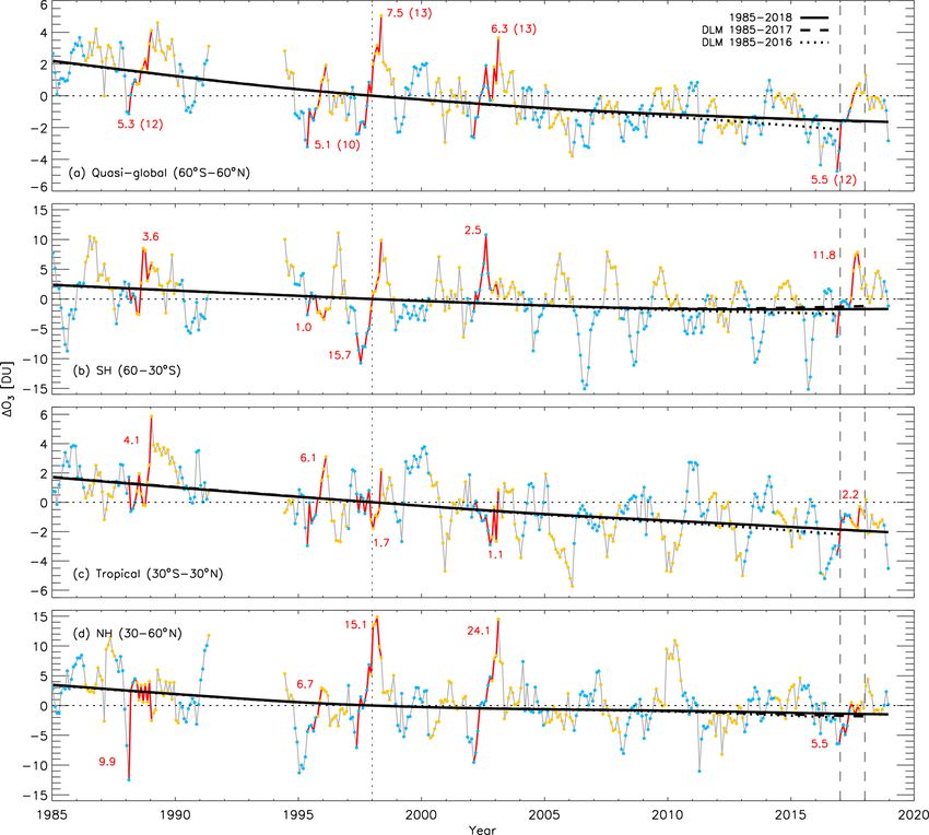
Figure 2. Lower stratospheric partial column ozone anomalies: (a) quasi-global (60◦ S–60◦ N), (b) Southern Hemisphere (60–30◦ S, 147–
30 hPa), (c) tropics (30◦ S–30◦ N, 100–30 hPa), and (d) Northern Hemisphere (30–60◦ N, 147–30 hPa). The DLM non-linear trend is shown
for 1985–2016 (dotted), 1985–2017 (dashed), and 1985–2018 (solid). Red lines represent contiguous periods identified in the quasi-global
anomalies exceeding 90 % of the magnitude of the November 2016 to October 2017 change within a 13-month period; the DU changes are
written above or below each period; red periods in (b–d) are those identified in (a). Coloured dots are plotted on each time series when the
QBO at 30 hPa is either in an easterly (yellow) or westerly (blue) phase. The 3-year period following the eruption of Mt. Pinatubo, June 1991
to May 1993, has been removed. Figures for the whole, upper, and middle stratosphere are provided in Figs. S2–S4 in the Supplement.
crease occurring within a 13-month period. The decomposed 3.3 Contribution of QBO to midlatitude ozone
time series (Fig. 2b–d) show that the large increases in the variability
SH are “normal”, occurring regularly. They also occur in the
NH, but not as regularly, and the tropical variability is much
smaller than the midlatitude variance. In addition to the large Chipperfield et al. (2018) convincingly showed that the ma-
increases, there are also comparatively large negative swings jority of post-1997 quasi-global lower stratospheric ozone
in both SH and NH time series – one in the NH beginning in variability in Fig. 2a was dynamically controlled, specifically
2002 exceeds 24 DU. In the following section we argue that in the lower stratosphere where the lifetime of ozone is long.
these large, rapid changes are driven by a non-linear seasonal Given that the contributions from each subregion (Fig. 2b–d)
QBO effect. add up to the quasi-global change in 2017, it is reasonable
to assume that dynamics controls much of the sub-decadal
variability there too. The peaks (or troughs) in the SH are
Atmos. Chem. Phys., 19, 12731–12748, 2019 www.atmos-chem-phys.net/19/12731/2019/W. T. Ball et al.: Stratospheric ozone sensitivity 12737
Figure 3. (Upper row) Histograms of ozone anomalies relative to the DLM non-linear trend line in Fig. 2 for months when the QBO at
30 hPa is either in an easterly (yellow) or westerly (blue) phase: (a) quasi-global (60◦ S–60◦ N), (b) Southern Hemisphere (60–30◦ S, 147–
30 hPa), (c) tropics (30◦ S–30◦ N, 100–30 hPa), and (d) Northern Hemisphere (30–60◦ N, 147–30 hPa). (Lower row) Difference between
QBO easterly and westerly histograms from the upper row.
2–3 years apart. The QBO has a similar periodicity and is To clarify this further, in Fig. 4 all 34 years in the 1985–
known to have the largest interannual dynamical impact on 2018 period are split into 13-month periods starting in Jan-
ozone in the stratosphere (see Gray and Pyle, 1989; Zerefos uary for the SH (Fig. 4a, b) and July for the NH (Fig. 4c, d),
et al., 1992, and Toihir et al., 2018, and references therein). i.e. a few months prior to the onset of winter in the respec-
Labelling each month in Fig. 2 with the 30 hPa QBO easterly tive hemisphere. The latitudes plotted are refined to isolate
or westerly phase with yellow or blue dots respectively, re- clearer signals for 50–30◦ S (Fig. 4a), 30–50◦ N (Fig. 4c),
veals that the large SH negative anomalies are almost always and 10◦ S–10◦ N (Fig. 4b, d). This refinement reduces the
associated with a westerly phase, whereas positive anomalies influence of polar variability on the 30–50◦ band, and iso-
are associated with an easterly phase; Bodeker et al. (2007) lates the equatorial region to where the QBO variability is
previously identified large SH negative anomalies in 1985, strongest. We note that the act of forming partial columns of
1997, and 2006 and related these to the QBO westerly phase. ozone may reduce the integrated variability compared with
This also appears to be the case in the NH, but the variabil- counter-varying layers that would otherwise be resolved by
ity is less regular, unsurprisingly as the NH stratosphere is pressure level. We find the use of the QBO phase at 15 hPa
known to have additional variability as a consequence of also better separates the events in this additional analysis.
greater sea–land contrast and more orography than in the We find negative and positive ozone excursions in the lower
SH. Thus, the NH exhibits stronger large-scale wave activity stratosphere become clear in 13-month segments when they
and, consequently, polar vortex and stratospheric variability are bias-shifted to zero in March (Fig. 4a, b) and Septem-
(see Butchart, 2014 and Kidston et al., 2015 and references ber (Fig. 4c, d) and then colour coded according to their QBO
therein). Equatorial variability in ozone related to the QBO phase in April or October respectively (vertical dotted line).
phase at 30 hPa shows the opposite behaviour to that at mid- The largest deviations are found to occur 4 or 5 months later
latitudes: decreases in ozone generally appear to occur with (vertical dashed line), at the onset of hemispheric autumn
the easterly phase and vice versa, and the return from max- (Holton and Tan, 1980; Dunkerton and Baldwin, 1991). It
imum excursion (i.e. the sign of the gradient) appears to be is also interesting to note that the only large, positive QBO
more related to the change in phase. westerly anomaly that peaks 4 months later, in either hemi-
Histograms of the ozone anomalies relative to the DLM sphere, occurs in the SH in 2002. This year is famous for
trend line for each QBO phase at 30 hPa are shown in the having the only observed sudden stratospheric warming in
upper row of Fig. 3. The shift in the histogram between QBO the SH, and indicates that while the QBO phase appears to
phases is clear in the SH. The NH displays little shift, again dominate this distribution of anomalies, other processes can
likely related to other drivers influencing NH ozone changes, also sometimes dominate.
although the extremes show a similar phase separation to We reiterate that the separation of positive and negative
that in the SH. The difference between the QBO easterly anomalies into those related to easterly or westerly QBO
and westerly histograms are shown in the bottom row, and phases is clearest for the SH (Fig. 4a) and the corresponding,
elucidate the correlation between the QBO state and ozone opposing, equatorial changes (Fig. 4b). The anti-correlated
anomalies. behaviour of anomalies between midlatitude and equatorial
regions is consistent with previous studies investigating the
www.atmos-chem-phys.net/19/12731/2019/ Atmos. Chem. Phys., 19, 12731–12748, 201912738 W. T. Ball et al.: Stratospheric ozone sensitivity Figure 4. Lower stratospheric partial column ozone at (a) 50–30◦ S, (b, d) 10◦ S–10◦ N, and (c) 30–50◦ N. Each line represents a 13-month period starting in January (a, b) or July (c, d), all bias-shifted to zero in March (a, b) or September (c, d) and colour coded by the state of the QBO at 15 hPa in April (a, b) or October (c, d) so that QBO easterly phases are yellow and the westerly phases are blue. The period covering November to December 2016 is highlighted as a dotted red line, whereas January to November 2017 is dashed red line. relationship between the QBO and midlatitude ozone vari- The 2017 increase is highlighted in Fig. 4, with Novem- ability (e.g. Zerefos et al., 1992; Randel et al., 1999; Strahan ber 2016 to January 2017 shown as a dotted red line, and et al., 2015). We summarise the dynamical concept, in the January to October 2017 as a dashed red line. Focusing on context of these results, in the following (see Baldwin et al., Fig. 4a in the SH, the increase onset during the easterly 2001 and Choi et al., 2002 for detailed discussion). The QBO phase is large, but as noted earlier larger excursions have oc- consists of downward-propagating equatorial zonal winds; in curred before at regular intervals (Fig. 2). A prolonged west- the lower stratosphere this consists of a westerly above an erly phase, following the breakdown of the expected QBO easterly, or vice versa. A westerly above an easterly (i.e. the pattern in 2016 (Osprey et al., 2016; Newman et al., 2016; 15 hPa QBO is westerly as identified by blue lines in Fig. 4) Tweedy et al., 2017), may have contributed to a suppressed leads to a shear that induces an anomalous downward motion level of ozone in 2016 (note the single orange dot in 2016 of air, and adiabatic warming (Fig. 1 of Choi et al., 2002) and in Fig. 2a signifying a brief easterly QBO phase). The ar- also leads to an anomalous increase in ozone. For an easterly rival of the easterly phase proper in 2017 led to the ozone above a westerly, this leads to anomalously rising air and adi- increase at midlatitudes. The westerly phase at 30 hPa began abatic cooling along with an associated ozone decrease. An in late 2018 and ozone should, barring no further QBO break- Equator-to-midlatitude circulation forms to conserve mass down, decrease again in 2019 in the SH midlatitudes; the last (Randel et al., 1999; Polvani et al., 2010; Tweedy et al., 3 months of 2018 hint at such a decrease (Fig. 2). 2017). At subtropical and midlatitudes, the return of this Despite this variability, Fig. 1 indicates that the lower meridional circulation draws ozone-rich air from above down stratospheric negative trends in ozone could already be iden- into ozone-poor regions, anomalously enhancing ozone there tified throughout the lower stratosphere before, and after, (yellow, Fig. 4a, c). When easterlies lie over westerlies (blue, 2016. As such, the QBO breakdown event is likely not the Fig. 4), the opposite circulation is set up, and ozone anoma- primary cause of the negative ozone trends reported by Ball lies reverse. et al. (2018), but does appear to affect the robustness of the Atmos. Chem. Phys., 19, 12731–12748, 2019 www.atmos-chem-phys.net/19/12731/2019/
W. T. Ball et al.: Stratospheric ozone sensitivity                                                                               12739

trend depending on the end year. We will investigate this end-          a good example of the inadequacy of using linear trends to
year sensitivity in Sect. 3.5.                                          describe these data. As the DLM-estimated changes in ozone
                                                                        relative to 1998 in years prior to 2010 are essentially unaf-
3.4   Latitude-integrated lower stratospheric ozone                     fected by the addition of 2017 and 2018, the data show ro-
      trend estimates                                                   bustly that lower stratospheric ozone did continue to decrease
                                                                        until at least 2010 in all regions. We speculate that the shift
While Chipperfield et al. (2018) applied ordinary least                 back to a QBO westerly phase will again decrease ozone at
squares trend fits to time series using a single linear trend,          midlatitudes in 2019 (which appears to have begun in Oc-
this cannot be compared to multivariate regression ap-                  tober 2018, see Fig. 2). If that happens, it is possible that
proaches, e.g. DLM and MLR. This is because the former                  the non-linear trend estimates will likely decrease again, and
simply asks what the trend in the data is, regardless of the            the emergent 2013 minimum in the DLM non-linear trend
forcing agents, whereas the latter attempts to separate known           estimate seen in Fig. 2b is likely to shift to a later date or
(usually quasi-periodic) drivers to distil out the trend that has       disappear.
(usually unknown) drivers of its own. The DLM non-linear
trend estimates presented here are the first multivariate anal-         3.5   Sensitivity of DLM trends to the end year and
ysis applied to ozone time series that include the large ozone                non-linear seasonal QBO effects
increase witnessed in 2017. It is important to clearly state
that long-term trends cannot be compared with single-year               As midlatitude ozone excursions depend on the QBO sea-
changes and, indeed, the processes governing each timescale             sonal interaction, i.e. the QBO phase relative to the time of
are likely quite different. While large short-term increases            year, this is a non-linear mode of variability. Without predic-
will likely bias the whole trend-line for that period under             tors to represent this non-linear behaviour, linear regression
MLR analyses (with piecewise linear and independent lin-                models (including both DLM and MLR) cannot capture these
ear trends – PWLT or ILT), DLM promises to be more robust               excursions and the variability can leak into, and bias, other
in the sense that asymmetric fluctuations will only influence           predictors. Most importantly, this bias may include the trend
part of the smooth trend over a timescale fixed by the smooth-          component of the regression model. In this section we exam-
ness parameter σtrend that controls how rapidly the trend is            ine the magnitude of this effect via a sensitivity analysis of
allowed to evolve (see Ball et al., 2017 and Fig. S1).                  the DLM trends to the end date of the data, both spatially and
    The DLM trends in lower stratospheric ozone estimated               with partial columns.
over 1985–2018 in Fig. 2 continue to be negative, monotonic                Due to the magnitude of the midlatitude, seasonally de-
trends up to 2018 in the quasi-global, tropical, and NH re-             pendent QBO ozone variability on short (2- to 3-year)
gions, while the SH trend reaches a minimum in ∼ 2013 be-               timescales, ILT or PWLT applied to the relatively short post-
fore slowly rising. All integrated regions suggest that mean            1997 time series will be sensitive to these large swings in
ozone remains below the 1998 level (see Table 13 ), although            ozone. For the smooth DLM trends in contrast, we expect
the probability of an overall decrease is 99 % in quasi-global          that the last few years of the curve will be primarily affected,
ozone, dominated by the tropics (99 %), with probabilities              with the rest of the trend being stable. We demonstrate the
of a decrease of 80 % and 76 % in the SH and NH respec-                 impact on DLM in Fig. 5, where the partial column regions as
tively. Except in the SH, monotonic downward trends remain,             presented in Ball et al. (2018) are shown for 10◦ bands, and
with the addition of 2 years only affecting the gradient of the         quasi-globally (right column), over the whole stratospheric
monotonic trends (compare the dotted line for the year end-             column (top), as well as the upper, middle, and lower strato-
ing in 2016, with the dashed line for 2017 and solid line for           sphere. We show DLM curves estimated from six periods
2018 in Fig. 2). This agrees with Chipperfield et al. (2018),           that start in 1985 and end in 2013–2018, as in Fig. 1. All
who suggested that the large rapid increase in 2017 affected            curves are bias shifted to zero in 1998. This provides a vi-
trends, although this was mainly in the SH and has subse-               sualisation of the sensitivity of the non-linear trends to the
quently showed little change over 2018. However, it has done            end year (and hence also the large resurgence in ozone in
little to reduce the overall probability of a decrease in the           2017). The uncertainties associated with a change between
quasi-global time series (99 %). Furthermore, the shape of              1998 and the end year are presented in Fig. 6 with 95 % (dark
the DLM curve is only affected near the end years, such that            grey shading) and 99 % credible intervals. The results specif-
the period away from the end date is relatively insensitive to          ically for the 1998–2018 change are combined and presented
a change in the end year and becomes “locked-in”4 . This is             in Fig. 7 as probability distributions, in the same manner as
                                                                        in Fig. 2 of Ball et al. (2018), where blue and red colours
   3 An extended Table S1 in the Supplement provides changes in
                                                                        represent negative and positive changes respectively, and the
DU (%) and percent per decade for 1985–2018, 1985–1997, and
                                                                        numbers above each distribution are the probability of the
1998–2018.
   4 In contrast, for MLR analyses, the entire trend-line is impacted   change (fraction of the probability distributions) being nega-
by changes in the end year (Frith et al., 2014; Weber et al., 2018;
                                                                        tive.
Keeble et al., 2018).

www.atmos-chem-phys.net/19/12731/2019/                                                Atmos. Chem. Phys., 19, 12731–12748, 2019
12740 W. T. Ball et al.: Stratospheric ozone sensitivity
Table 1. Absolute change between 1998 and 2018 in Dobson units, and probability (in parentheses) of a positive or negative change in ozone
(%) for integrated regions of the stratosphere. Standard text indicates that ozone changes are negative, italic text indicates positive changes,
and bold text indicates probabilities exceeding 90 %.
Region 60–30◦ S 50–30◦ S 30◦ S–30◦ N 20◦ S–20◦ N 30–50◦ N 30–60◦ N 50◦ S–50◦ N 60◦ S–60◦ N
Whole −0.5 (57) −0.4 (56) –1.9 (95) –2.5 (95) −3.2 (83) −2.6 (77) −1.1 (86) −1.1 (86)
Upper +0.8 (100) +0.8 (99) +0.7 (96) +0.6 (85) +0.6 (92) +0.6 (96) +0.8 (100) +0.8 (100)
Middle +0.7 (78) +0.8 (78) –0.7 (94) –0.9 (95) −0.5 (73) −0.5 (72) −0.4 (81) −0.2 (73)
Lower −1.6 (80) −1.7 (82) –2.1 (99) –2.1 (98) −1.9 (82) −1.5 (76) –1.8 (99) –1.7 (99)
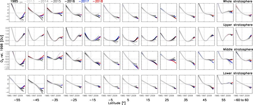
From the panels of Fig. 5, it is clear that ozone trends in in a local minimum emerging in the non-linear trend curve
the middle stratosphere exhibit the largest sensitivity to the around 2013. As such we can infer that additional data are
end year, and the uncertainties in the change from 1998 are unlikely to affect the inferred change of ozone in 2013, rel-
consistently large (Fig. 6). Quasi-globally the middle strato- ative to 1998, or push the minima to earlier dates, because
sphere change since 1998 is negative for all end years, but the affecting end year moves further away with more data.
does not exceed 95 % probability. The upper stratosphere is However, subsequent data might once again push the changes
also sensitive to the end year in the tropics (Fig. 5), and the since 1998 to lower levels, e.g. if midlatitudes do respond to
end year shifts the estimated ozone change from negative to a westerly phase QBO with ozone reducing sharply as it has
positive with increasing end year, although the uncertainty done in the past (Fig. 2). We expand the idea of inferring
always remains large (Fig. 6). At midlatitudes uncertainties the likely earliest minimum using the DLM with spatially re-
in the change of upper stratospheric ozone since 1998 are solved data in the Supplement.
smaller, but there has been a general shift towards more posi-
tive and significant increases, which is more clearly reflected 3.6 Update on ozone profiles
in the SH and quasi-global estimates.
The evolution of the lower and whole stratospheric non- Briefly, in Fig. 8, we provide updated ozone change pro-
linear ozone trends mimic each other. South of 30◦ S, the files for 1998–2018 using the standard latitudinal ranges for
end points of the negative changes have quickly increased the SH (60–35◦ S), the tropics (20◦ S–20◦ N), and the NH
in 2017 and 2018 relative to 1998, although they remain neg- (35–60◦ N) (WMO, 2014, 2018; Steinbrecht et al., 2017;
ative in the lower stratosphere. At latitudes north of 30◦ S, Petropavlovskikh et al., 2019). Figure 8, also includes 1998–
the addition of 2017 and 2018 has made little difference 2016 and 1998–2017 profiles for comparison and shows that,
to the monotonic ozone decline and for 50–60◦ N, where for 1998–2018, confidence in an upper stratospheric ozone
changes are flat, the additional years make little difference. recovery from ODSs is clear for all latitude bands, includ-
The quasi-global lower stratospheric ozone continues to ex- ing the tropics where it has previously remained below the
hibit a monotonic decline that is still highly confident with 95 % significance levels. The lower stratosphere shows neg-
99 % probability (Fig. 7 and Table 1), and ozone abundances ative ozone changes at almost all levels, although these gen-
integrated over the whole stratosphere continue to remain erally do not exceed a probability of 95 %.
lower in 2018 than in 1998, although this is now with a Ball et al. (2018), and Fig. 7 in this paper, indicate that
probability of 86 %; these trends are dominated by the tropi- the 50–60◦ zonal means in both hemispheres show little
cal contribution (58 %, latitude weighted) to the quasi-global ozone change in the lower stratosphere over the last 21 years,
change, whereas the NH and SH contribute 21 % each. Even whereas the tropical regions out to 30◦ show a strong de-
so, the NH changes do not appear affected by the recent large crease. By modifying the latitudinal extent of the profiles
seasonally dependent QBO variability. slightly, so that midlatitudes cover 30–50◦ to exclude 50–
Figure 5 also confirms that the gradients of the non-linear 60◦ and the tropics are widened to 30◦ S–30◦ N to include
curves are only affected by unmodelled variance in years the subtropics, the modified profiles are presented in Fig. 9.
close to the end points, typically within the last 5 years of This provides some measure of the sensitivity to the latitu-
the partial column time series considered here. The shape of dinal ranges chosen. Now we see the tropics show close to
the DLM curves prior to the final 5 years of the DLM curves 95 % confidence of an ozone decrease at all tropical lower
are largely unaffected. Indeed, even with the large ozone in- stratospheric pressure levels, and there is increased confi-
crease in 2017 in the SH, we see that all trend-curves agree dence of an ozone reduction in the midlatitude lower strato-
well prior to 2010. This is also true in other panels, e.g. the sphere. Furthermore, the inclusion of higher latitude regions
middle stratosphere and tropical upper stratosphere. In the (20–30◦ ) reinforces the tropical upper stratosphere ozone in-
upper stratosphere the recovery onset remains robust, but in crease.
the SH lower stratosphere the large increase in 2017 results An upper stratospheric increase is the expected result from
long-term stratospheric chlorine reductions, a direct conse-
Atmos. Chem. Phys., 19, 12731–12748, 2019 www.atmos-chem-phys.net/19/12731/2019/W. T. Ball et al.: Stratospheric ozone sensitivity 12741 Figure 5. The partial column ozone non-linear trends estimated as a function of end year (2013 to 2018; dark to light colours), for each 10◦ latitude and quasi-global (left to right) and the whole, upper, middle, and lower stratosphere (top to bottom). Each sub-panel covers 1985–2018 and all curves are bias corrected to January 1998 (horizontal and vertical dotted lines). Uncertainties for each 1998 to end-year change are given in Fig. 6. Figure 6. The partial column ozone changes between 1998 and the end year from 2013 to 2018 (x axis of each sub-panel) from the non-linear trends, as in Fig. 5. Dark and light shading represent the respective 95 % and 99 % credible intervals. quence of the Montreal Protocol and its amendments, al- as dynamical changes (Wargan et al., 2018). These results though we do not explicitly attribute the cause of the increase once again reinforce the conclusion that only the SH is af- to that here (for more on attribution see, for example, WMO, fected by the 2017 ozone increase (lower stratosphere), that 2018). Indeed, the Montreal Protocol and its amendments the Montreal Protocol appears to be working (upper strato- will have been effective in reducing ozone losses through- sphere), and that the decreases in the lower stratosphere at out the atmosphere via reductions in CFC emissions, HCFCs, tropical and NH latitudes remain in place, but are not yet and other ODSs. The lack of a positive trend since 1998 in the fully understood. lower stratosphere, as opposed to the one clear in the upper stratosphere, is likely the consequence of other factors such www.atmos-chem-phys.net/19/12731/2019/ Atmos. Chem. Phys., 19, 12731–12748, 2019
12742                                                                               W. T. Ball et al.: Stratospheric ozone sensitivity

Figure 7. Posterior distributions (shaded) for the 1998–2018 partial column ozone changes. (Top) whole stratospheric column, (middle)
upper, and (bottom) lower stratosphere in 10◦ bands for all latitudes (left) and integrated from 60◦ S–60◦ N (“Quasi-global”, right). The
stratosphere extends deeper at midlatitudes than at equatorial latitudes (marked above each latitude). Numbers above each distribution
represents the distribution percentage that is negative; colours are graded relative to the percentage distribution (positive, red hues, with
values < 50; negative, blue).

4   Conclusions                                                          tion and long-range studies of ozone, but different types ex-
                                                                         ist. Free-running CCMs generate their own model-dependent
                                                                         internal climate and variability. Chemistry transport mod-
Here, we have extended and analysed the BASICSG strato-
                                                                         els (CTMs) use wind, temperature, and surface pressure
spheric ozone composite from Ball et al. (2018) by 2 years
                                                                         fields fully prescribed by reanalyses. Furthermore, specified-
to cover 1985–2018. BASICSG merges two composites,
                                                                         dynamics CCMs (SD-CCMs) use reanalyses to nudge the in-
SWOOSH and GOZCARDS. We perform a set of sensitiv-
                                                                         ternally generated variability of the model closer to the his-
ity tests, using dynamical linear modelling (DLM), on the
                                                                         torical variability in the real atmosphere while attempting to
post-1997 trend estimates to understand the impact of a re-
                                                                         retain model-dependent processes and internal consistency.
cently reported, large increase in modelled ozone in the lower
                                                                         CTMs and SD-CCMs can be useful for attributing histori-
stratosphere in 2017 (Chipperfield et al., 2018), following al-
                                                                         cal changes in ozone to evolving concentrations of CO2 and
most 2 decades of persistently decreasing ozone.
                                                                         ODSs (Solomon et al., 2016), or the Sun (Ball et al., 2016),
   The aim of this work is to assess the current state of, and
                                                                         by accounting for dynamical variability in observations.
trends in, stratospheric ozone. Improved knowledge of such
                                                                            A recent study (Chipperfield et al., 2018) used a CTM
trends, and the relevant forcing mechanisms and associated
                                                                         to reconstruct the ozone time series beyond the observa-
variability, will help to better constrain CCM projections of
                                                                         tional record available at the time to 2017 and found that
ozone to the end of the 21st century. Chemistry models re-
                                                                         the CTM simulated a lower stratospheric ozone increase
solving the stratosphere are one of the best tools for attribu-

Atmos. Chem. Phys., 19, 12731–12748, 2019                                                 www.atmos-chem-phys.net/19/12731/2019/
W. T. Ball et al.: Stratospheric ozone sensitivity 12743 Figure 8. The ozone profiles for 1998 to an end year of 2016 through 2018 (see legend) in the Southern Hemisphere (60–35◦ S), the tropics (20◦ S–20◦ N), and the Northern Hemisphere (35–60◦ N). Shading is for 2016 only. Uncertainties are 95 % credible intervals. Pink lines indicate the boundaries of partial columns in other figures. Figure 9. As for Fig. 8, but for the 50–30◦ S (SH), 30◦ S–30◦ N (tropics), and 30–50◦ N (NH) regions. in 2017 back to 1998 levels. This increase was attributed of the long-term decreases or the 2017 increase. Here, we to dynamical variability. Indeed, chemistry and photochem- show that the 2017 increase simulated by the CTM (Chip- istry play a dominant role over dynamical perturbations in perfield et al., 2018) was more than 60 % larger than that ob- the upper stratosphere as ozone lifetimes are short (∼ days), served, and that the 1998–2017 and 1998–2018 (Fig. 1e and while ozone lifetimes of ∼ 6–12 months in the lower strato- f) change remains negative (60◦ S–60◦ N), and significant in sphere mean that Equator-to-midlatitude transport of similar the tropics and some subregions of the NH (Fig. 1f). Nei- timescales plays an important (dominant) role there (London, ther free-running CCMs (WMO, 2014), nor SD-CCMs (Ball 1980; Perliski et al., 1989; Brasseur and Solomon, 2005). et al., 2018), have so far been demonstrated to accurately re- CTMs can provide insight as to whether the changes might produce the long-term changes estimated from observations be driven by photochemistry, chemistry, or dynamics. How- in lower stratospheric ozone (Fig. 6). ever, because the dynamical fields are prescribed, the CTM The effect of the ozone increase in 2017 was small and the cannot provide insight into the underlying dynamical driver probability of an overall ozone decrease in the lower strato- www.atmos-chem-phys.net/19/12731/2019/ Atmos. Chem. Phys., 19, 12731–12748, 2019
12744                                                                         W. T. Ball et al.: Stratospheric ozone sensitivity

sphere remains at 99 % for 1998–2018 (−1.7 DU, or 2.0 %;              Future projections tend to focus on how stratospheric
see Table S1). We note that the lower stratospheric ozone          ozone will evolve under a given global warming scenario.
trends are dominated by the tropical regions (30◦ S–30◦ N)         This is important given that anthropogenic GHG emissions
where the decrease is robust to the end year over 2013–2018,       that are changing the climate may impact interannual dynam-
with a probability of 99 % (−2.1 DU, −3.5 %) that it was           ical variability in the stratosphere (Osprey et al., 2016; New-
lower in 2018 than in 1998. Nevertheless, midlatitudes out         man et al., 2016; Tweedy et al., 2017). Changes are also ex-
to 50◦ N also indicate that the decrease persists (−1.9 DU,        pected in the large-scale circulation of the stratosphere, and
−1.7 %). We also find that the 2017–2018 addition enhances         these are likely to modify future distributions of ozone (Chip-
the estimated magnitude of the upper stratospheric ozone           perfield et al., 2017). Further, ozone is not a passive tracer,
positive trend, but that the quasi-global (60◦ S–60◦ N) ozone      and the large-scale long-term changes in ozone are expected
layer still displays a reduction since 1998, although the con-     to feedback on the aforementioned dynamics (Li et al., 2018;
fidence in this has reduced from 95 % in 2016 (Ball et al.,        Polvani et al., 2018; Abalos et al., 2019). Such a feedback
2018) to 86 % in 2018 (−1.1 DU, −0.4 %). Given the high            has been demonstrated, most notably, in the SH following
probability of a decrease in tropical middle (94 %) and lower      ozone depletion and the growth of the ozone hole (WMO,
(99 %) stratospheric ozone, the whole tropical stratospheric       2014, 2018). Now, as ozone is expected to recover in the
ozone column indicates a highly probable decrease (95%)            coming decades, the dynamics of the stratosphere are also
over 1998–2018 (−1.9 DU, −0.8 %).                                  expected to respond. The overall future expectations are that
   In general, uncertainties on changes since 1998 in partial      total column ozone levels will return to 1980s levels glob-
columns have changed little over 2013–2018 (Fig. 6), a result      ally by ∼ 2050, in the Antarctic by 2100, and by ∼ 2030 and
likely due to the large fraction of unaccounted for variance in    ∼ 2050 in northern and southern midlatitudes respectively.
the standard set of predictors used in regression analysis. Our    The midlatitudes are expected to continue on to a “super-
analysis shows that ozone continued to decrease until a mini-      recovery”, i.e. that ozone will be higher by the end of the
mum in at least 2013 in the SH, and has continued to decrease      21st century than prior to 1980s levels (Dhomse et al., 2018;
at all latitudes north of 30◦ S. By comparing the phase of the     WMO, 2014, 2018), although this is predicated on future
QBO with large, 2–3 year interannual variability at midlati-       scenarios of the decreases of hODSs continuing as expected
tudes, the implication is that these large midlatitude changes     (Montzka et al., 2018). However, it is not clear whether the
are related to the seasonal-dependence of ozone on the QBO,        recent increase in SH lower stratospheric ozone will remain
i.e. a non-linearity. If true, this could explain why regres-      at higher levels or will reduce again in 2019 as the QBO shifts
sion models cannot capture this variability, as such non-linear    to a westerly phase, nor why the NH continues to show a per-
behaviour is not included. The clarification of the origin of      sistent decrease. Nonetheless, we note that the signal is small
these large midlatitude changes – occurring every few years        compared with the (i) large interannual variability, (ii) pre-
– is a high priority.                                              2000 changes induced by ozone-depleting substances, and
   CCMs are consistent in the sign of their projections, al-       (iii) ozone loses that would have occurred without the Mon-
though lower stratospheric ozone variability can differ with       treal Protocol being enacted.
observations and there is a large spread in their sensitivity to      The ongoing negative trend of ozone in the lower strato-
hODSs (Douglass et al., 2012, 2014), and therefore their re-       spheric component of the total column also continues to pose
turn dates, i.e. a return of ozone to the level it was in 1980     a problem for global trends in tropospheric ozone. If tropo-
(WMO, 2014; Dhomse et al., 2018; WMO, 2018). CCMs do               spheric ozone has really increased over the last 2 decades,
a good job on many timescales, but due to historically dif-        and stratospheric ozone was not decreasing or remained flat,
ferent internal variability, and parameterised sub-grid-scale      then some component of the total column ozone must have
processes and numerical diffusion, behaviour in some re-           been decreasing to balance the ozone budget as it appears that
gions may not be well-reproduced (SPARC/WMO, 2010). It             total column ozone has remained steady over the past 5–10
is clear from modelling studies that pre-Montreal Protocol         years. Alternatively, it is possible that the solution simply lies
ozone decreases can be attributed to ODS increases (WMO,           in very large observational uncertainties (Harris et al., 2015;
2014), and SD-CCMs and CTMs generally reproduce the                Gaudel et al., 2018; Petropavlovskikh et al., 2019) and/or the
Antarctic ozone hole well (Solomon et al., 2016). The halt in      inadequacies of linear regression techniques to attribute vari-
ODS-related ozone losses as a result of the Montreal Proto-        ability and identify trends. In addition to potential future im-
col and its amendments, and an initial recovery from ODSs          provements in merged observational records, this calls for a
in total column ozone is almost universally reproduced by          community push to improve detection and attribution tech-
CCMs (SPARC/WMO, 2010), as is the upper stratospheric              niques to solve an issue that is of great importance to the
ozone recovery. However, negative ozone trends since 1998          health of society, the biosphere, and the climate.
in the lower stratosphere have not been demonstrated to be
simulated in models in the midlatitudes, most notably in the
NH.

Atmos. Chem. Phys., 19, 12731–12748, 2019                                          www.atmos-chem-phys.net/19/12731/2019/
You can also read