Streambank Erosion and Related Geomorphic Change in Tuolumne Meadows, Yosemite National Park, California - USGS Publications Repository
←
→
Page content transcription
If your browser does not render page correctly, please read the page content below
Prepared in cooperation with the National Park Service

Streambank Erosion and Related Geomorphic Change in
Tuolumne Meadows, Yosemite National Park, California

Scientific Investigations Report 2021–5025

U.S. Department of the Interior
U.S. Geological Survey
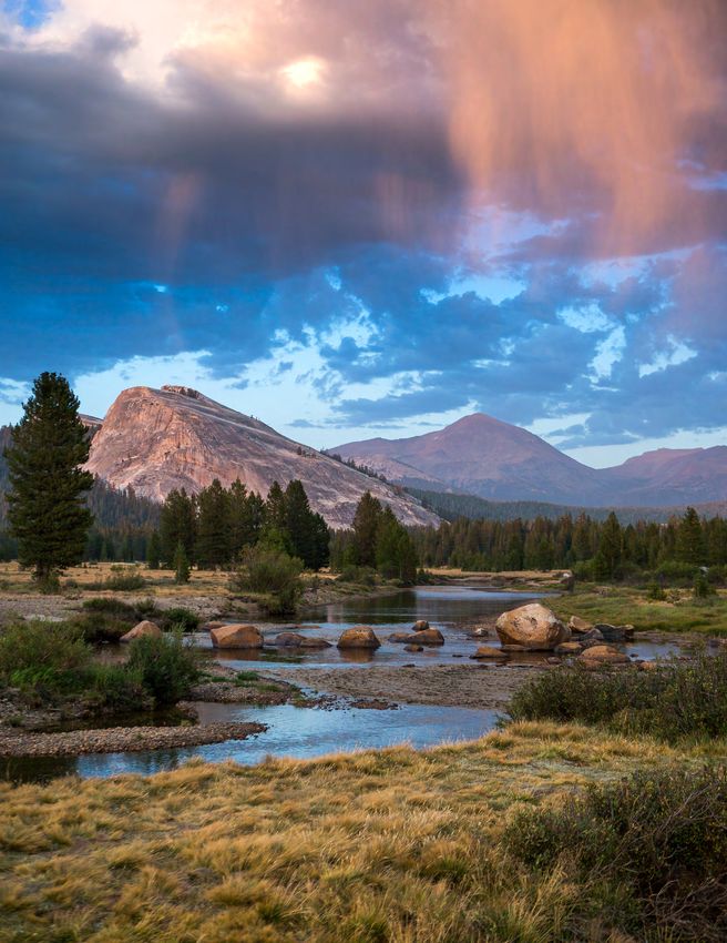
Front Cover. Photograph of Tuolumne River in Tuolumne Meadows, California, looking east from erosion zone 5 as defined in this report with
Lembert Dome and Mount Gibbs visible in the background . Photograph by Ryan Alonzo, titled Tuolumne Virga, used with permission.

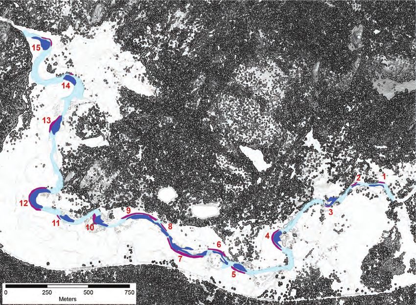
Back cover. (1) U.S. Geological Survey photograph of the Tuolumne River in Tuolumne Meadows, California, looking southeast from just west of
erosion zone 5 as defined in this report with Mammoth Peak visible in the background. (2) U.S. Geological Survey photograph of the Tuolumne River
in Tuolumne Meadows, California, looking west from erosion zone 7 as defined in this report with Pothole Dome and Fairview Dome visible in the
background.
Streambank Erosion and Related Geomorphic Change in
Tuolumne Meadows, Yosemite National Park, California

By Stephen B. DeLong, Alexandra J. Pickering, and Timothy Kuhn

Prepared in cooperation with the National Park Service

Scientific Investigations Report 2021–5025

U.S. Department of the Interior
U.S. Geological Survey
U.S. Geological Survey, Reston, Virginia: 2021

For more information on the USGS—the Federal source for science about the Earth, its natural and living resources,
natural hazards, and the environment—visit https://www.usgs.gov or call 1–888–ASK–USGS (1–888–275–8747).
For an overview of USGS information products, including maps, imagery, and publications,
visit https://store.usgs.gov.

Any use of trade, firm, or product names is for descriptive purposes only and does not imply endorsement by the
U.S. Government.

Although this information product, for the most part, is in the public domain, it also may contain copyrighted materials
as noted in the text. Permission to reproduce copyrighted items must be secured from the copyright owner.

Suggested citation:
DeLong, S.B., Pickering, A.J., and Kuhn, T., 2021, Streambank erosion and related geomorphic change in Tuolumne
Meadows, Yosemite National Park, California: U.S. Geological Survey Scientific Investigations Report 2021–5025,
87 p., https://doi.org/10.3133/sir20215025.

ISSN 2328-0328 (online)
iii

Preface
Tuolumne Meadows, in the high country of Yosemite National Park, California, is a renowned
natural and recreational resource noted for its scenic beauty, wildlife, and as a place of
peace and tranquility. It attracts large numbers of visitors from around the world, and its
importance is recognized by its designation as part of the Tuolumne Wild and Scenic River Final
Comprehensive Management Plan. In keeping with this designation, management decisions
are made with respect to biologic, geologic, cultural, scenic and recreational values with the
purpose of preserving the Tuolumne River in free-flowing conditions, and to protect water
quality. Part of the management plan is to monitor streambank dynamics in Tuolumne Meadows
and to make science-based decisions regarding management and restoration efforts. This report
provides scientific information towards these objectives.

Acknowledgments
The National Park Service (NPS) funded, collaborated on, and provided logistical support for this
project. The National Center for Airborne Laser Mapping and Greg Stock, NPS, were responsible
for the 2006 airborne laser swath mapping data, and OpenTopography which hosts and serves
the data to users. Kyle Juracek and Matthew Cashman provided very helpful and detailed
reviews of this report. Joseph Mason, William Otto, Nikita Avdievitch, Zachary Engle, and Sally
Keating provided field assistance. Jan van Wagtendonk and Peggy Moore facilitated use of the
U.S. Geological Survey research cabin in Yosemite National Park. Harrison Forrester provided
logistical support in Yosemite National Park. Zachary Engle assisted with figures. Rachel Hallnan
provided updated streamflow data.
iv

     Contents
     Preface............................................................................................................................................................iii
     Acknowledgments.........................................................................................................................................iii
     Abstract............................................................................................................................................................1
     Introduction.....................................................................................................................................................1
     Description of Tuolumne Meadows.............................................................................................................3
     Methods...........................................................................................................................................................4
          Field Surveys..........................................................................................................................................4
          Point Cloud Processing.........................................................................................................................6
          Airborne Lidar Data...............................................................................................................................6
          Generation of Derivative Products from Lidar Point Clouds...........................................................6
          Landscape Change Mapping...............................................................................................................8
          Streambank Mapping............................................................................................................................9
          Empirical Error Estimate Refinement Using Stable Landscape Areas.......................................10
     Results ............................................................................................................................................................10
          Vegetation Mapping............................................................................................................................10
          Streambank Mapping..........................................................................................................................11
          Zones of Active Streambank Migration and Landscape Change................................................11
          Details of Landscape Change at Erosion Zones.............................................................................13
                  Erosion Zone 1.............................................................................................................................14
                  Erosion Zone 2.............................................................................................................................18
                  Erosion Zone 3.............................................................................................................................22
                  Erosion Zone 4.............................................................................................................................26
                  Erosion Zone 5.............................................................................................................................31
                  Erosion Zone 6.............................................................................................................................35
                  Erosion Zone 7.............................................................................................................................40
                  Erosion Zone 8.............................................................................................................................45
                  Erosion Zone 9.............................................................................................................................49
                  Erosion Zone 10...........................................................................................................................53
                  Erosion Zone 11...........................................................................................................................57
                  Erosion Zone 12...........................................................................................................................61
                  Erosion Zone 13...........................................................................................................................67
                  Erosion Zone 14...........................................................................................................................71
                  Erosion Zone 15...........................................................................................................................75
     Discussion......................................................................................................................................................80
     Conclusions...................................................................................................................................................85
     References Cited .........................................................................................................................................86
v

Figures
    1.   Map of Tuolumne Meadows in Yosemite National Park, California, USA............................2
    2.   Maps of Tuolumne Meadows study area..................................................................................4
    3.   Slopeshade maps made from terrestrial laser scanner data of the study area from
         2016–2018........................................................................................................................................5
    4.   Maps of vegetation canopy height in Tuolumne Meadows derived from 2006
         airborne laser swath mapping and 2018 terrestrial laser scanning......................................7
    5.   Map of streambank willows and short vegetation along Tuolumne River derived
         from 2018 terrestrial laser scanning point clouds....................................................................8
    6.   Map of indistinct/stable and steep/active areas along the Tuolumne River.......................9
    7.   Maps depicting elevation changes from 2006 to 2018 in Tuolumne Meadows.................12
    8.   Map of polygons used to extract erosion and deposition volumes along the
         Tuolumne River.............................................................................................................................13
    9.   Lidar-derived maps showing location and classification of stream banks at
         erosion zone 1..............................................................................................................................15
   10.   Lidar-derived maps of vegetation at erosion zone 1..............................................................17
   11.   Photographs of erosion zone 1 in 2016....................................................................................18
   12.   Lidar-derived maps showing location and classification of stream banks at
         erosion zone 2..............................................................................................................................19
   13.   Lidar-derived maps of vegetation at erosion zone 2..............................................................21
   14.   Lidar-derived maps showing location and classification of stream banks at
         erosion zone 2..............................................................................................................................23
   15.   Lidar-derived maps of vegetation at erosion zone 3..............................................................25
   16.   Photographs of erosion zone 3 in 2016....................................................................................26
   17.   Lidar-derived maps showing location and classification of stream banks at
         erosion zone 4..............................................................................................................................27
   18.   Lidar-derived maps of vegetation at erosion zone 4..............................................................29
   19.   Photographs of erosion zone 4, 2016–2018.............................................................................30
   20.   Lidar-derived maps showing location and classification of stream banks at
         erosion zone 5..............................................................................................................................32
   21.   Lidar-derived maps of vegetation at erosion zone 5..............................................................34
   22.   Photographs of erosion zone 5 in 2016 and 2017....................................................................35
   23.   Lidar-derived maps showing location and classification of stream banks at
         erosion zone 6..............................................................................................................................36
   24.   Lidar-derived maps of vegetation at erosion zone 6..............................................................38
   25.   Photographs of erosion zone 6 in 2018....................................................................................39
   26.   Lidar-derived maps showing location and classification of stream banks at
         erosion zone 7..............................................................................................................................41
   27.   Lidar-derived maps of vegetation at erosion zone 7..............................................................43
   28.   Photographs of erosion zone 7 in 2016 and 2018....................................................................44
   29.   Lidar-derived maps showing location and classification of stream banks at
         erosion zone 8..............................................................................................................................46
   30.   Lidar-derived maps of vegetation at erosion zone 8..............................................................48
   31.   Photographs of erosion zone 8 in 2016....................................................................................49
   32.   Lidar-derived maps showing location and classification of stream banks at
         erosion zone 9..............................................................................................................................50
vi

     33.   Lidar-derived maps of vegetation at erosion zone 9..............................................................52
     34.   Photographs of erosion zone 9 in 2016....................................................................................53
     35.   Lidar-derived maps showing location and classification of stream banks at
           erosion zone 10............................................................................................................................54
     36.   Lidar-derived maps of vegetation at erosion zone 10............................................................56
     37.   Photographs of erosion zone 10 in 2016..................................................................................57
     38.   Lidar-derived maps showing location and classification of stream banks at
           erosion zone 11............................................................................................................................58
     39.   Lidar-derived maps of vegetation at erosion zone 11............................................................60
     40.   Photograph of erosion zone 11 in 2016....................................................................................61
     41.   Lidar-derived maps showing location and classification of stream banks at
           erosion zone 12............................................................................................................................62
     42.   Lidar-derived maps of vegetation at erosion zone 12............................................................64
     43.   Photographs of erosion zone 12 in 2016..................................................................................65
     44.   Lidar-derived maps showing location and classification of stream banks in
           erosion zone 13............................................................................................................................67
     45.   Lidar-derived maps of vegetation at erosion zone 13............................................................69
     46.   Photographs of erosion zone 13 in 2017..................................................................................70
     47.   Lidar-derived maps showing location and classification of stream banks at
           erosion zone 14............................................................................................................................71
     48.   Lidar-derived maps of vegetation at erosion zone 14............................................................73
     49.   Photographs of erosion zone 14 in 2018..................................................................................74
     50.   Lidar-derived maps showing location and classification of stream banks at
           erosion zone 15............................................................................................................................75
     51.   Lidar-derived maps of vegetation at erosion zone 15............................................................77
     52.   Photographs of erosion zone 15 in 2018..................................................................................78
     53.   Graph of streambank volumetric change rate versus sinuosity along the Tuolumne
           River channel measured at eroding streambanks.................................................................82
     54.   Graph of streambank retreat rate versus sinuosity along the Tuolumne River
           channel measured at migrating streambanks........................................................................83
     55.   Graph of streambank volumetric change rate (from mapping) versus sinuosity
           along the Tuolumne River channel...........................................................................................83
     56.   Graph of stream discharge along the Tuolumne River upstream of Tuolumne
           Meadows at gage “TUM” from 2006 to 2018..........................................................................84
vii

Tables
      1.   Lidar point cloud data used in this study...................................................................................5
      2.   Indication of vertical accuracy of DEMs of difference (DoDs) using apparently
           stable areas including highway, gravel roads, gravel hiking trails, and natural
           bedrock outcrops.........................................................................................................................11
      3.   Estimates of erosion and deposition at erosion zone 1 along Tuolumne River.................14
      4.   Estimates of erosion and deposition at erosion zone 2 along Tuolumne River.................22
      5.   Estimates of erosion and deposition at erosion zone 3 along Tuolumne River.................22
      6.   Estimates of erosion and deposition at erosion zone 4 along Tuolumne River.................26
      7.   Estimates of erosion and deposition at erosion zone 5 along Tuolumne River.................31
      8.   Estimates of erosion and deposition at erosion zone 6 along Tuolumne River.................39
      9.   Estimates of erosion and deposition at erosion zone 7 along Tuolumne River.................40
     10.   Estimates of erosion and deposition at erosion zone 8 along Tuolumne River.................45
     11.   Estimates of erosion and deposition at erosion zone 9 along Tuolumne River.................49
     12.   Estimates of erosion and deposition at erosion zone 10 along Tuolumne River...............53
     13.   Estimates of erosion and deposition at erosion zone 11 along Tuolumne River...............61
     14.   Estimates of erosion and deposition at erosion zone 12 along Tuolumne River...............66
     15.   Estimates of erosion and deposition at erosion zone 13 along Tuolumne River...............70
     16.   Estimates of erosion and deposition at erosion zone 14 along Tuolumne River...............74
     17.   Estimates of erosion and deposition at erosion zone 15 along Tuolumne River...............78
     18.   Rates of erosion at streambanks along Tuolumne River.......................................................79
     19.   Rates of sediment deposition on point and channel bars opposite eroding
           streambanks along Tuolumne River.........................................................................................80
     20.   Net volumetric change along entire surveyed reach of the Tuolumne River....................81
     21.   Sinuosity at zones of streambank erosion along Tuolumne River.......................................82

Conversion Factors
International System of Units to U.S. customary units
                Multiply                                              By                                             To obtain
                                                                   Length
 centimeter (cm)                                                  0.3937                            inch (in.)
 meter (m)                                                        3.281                             foot (ft)
 kilometer (km)                                                   0.6214                            mile (mi)
 meter (m)                                                        1.094                             yard (yd)
                                                                     Area
 hectare (ha)                                                     2.471                             acre
 hectare (ha)                                                     0.003861                          square mile (mi2)
                                                                  Flow rate
 cubic meter per year (m /yr)  3
                                                                  0.000811                          acre-foot per year (acre-ft/yr)
viii

       Datum
       Vertical coordinate information is referenced to the WGS84 Ellipsoid.
       Horizontal coordinate information is referenced to the North American Datum of 1983 (NAD 83).

       Abbreviations
       3D			             three dimensional
       ALSM			           Airborne laser swath mapping
       DEM			            Digital elevation model
       DoD			            DEMs of difference
       GPS			            Global Positioning System
       LoD			            level of detection
       NCALM		           National Center for Airborne Laser Mapping
       TLS			            Terrestrial laser scanning
Streambank Erosion and Related Geomorphic Change in
Tuolumne Meadows, Yosemite National Park, California
By Stephen B. DeLong1, Alexandra J. Pickering1, and Timothy Kuhn2
Abstract Introduction
Landscape change in Tuolumne Meadows, Yosemite Tuolumne Meadows is a large subalpine meadow in the
National Park, California, was characterized using data derived high-elevation part of Yosemite National Park, California (fig. 1).
from four lidar surveys: one airborne survey in 2006 and three It is situated at about 2,600 meters (m) above sea level, surrounded
terrestrial surveys in 2016, 2017, and 2018. These surveys were by iconic granodiorite domes, ridges, and peaks. The meadow is a
used to generate a better quantitative understanding of changes delicate ecological attraction made up of subalpine vegetation and
associated with fluvial processes along the reach of the Tuolumne erodible soils that have developed since glaciers receded between
River within Tuolumne Meadows. This research was performed 17,000 and 14,000 years ago. It is a focal area for visitation to
to provide a scientific basis for restoration and management Yosemite National Park. Visitor use, historical land use, and
decisions made by the National Park Service in accordance with natural processes may affect current conditions of Tuolumne
the Tuolumne Wild and Scenic River Final Comprehensive Meadows. It is thought that the ecological integrity (the ability of
Management Plan. A total of 15 reaches of the streambanks along the ecosystem to support ecological function, species diversity, and
the Tuolumne River in Tuolumne Meadows were subject to other characteristics similar to nearby ecosystems) of the meadows
measurable streambank erosion between 2006 and 2018. In these may be declining (Cooper and others, 2006; Buhler and others,
areas, streambank retreat rates ranged between 0 and 2.7 meters 2010). The Tuolumne Meadows reach is within a designated
per year (m/yr), recorded as an average retreat distance along the “scenic” reach and is managed according to the Tuolumne Wild
length of changing streambank position, with most retreat rates and Scenic River Final Comprehensive Management Plan and
being less than 0.50 m/yr. The highest streambank retreat rates Environmental Impact Statement (National Park Service, 2014).
are associated with a year of high spring streamflow in 2017. This plan—herein referred to as the Tuolumne River plan—guides
Based on the data available, it was concluded that deposition on management of the Tuolumne River by emphasizing preservation
channel and point bars balances streambank erosion over a period of its free-flowing conditions, protection of water quality, and
of 12 years along the Tuolumne River in Tuolumne Meadows. protection of its “outstanding remarkable values.”
As such, the river could be considered to be in a state of dynamic Within the framework of the Tuolumne River plan,
equilibrium during this period; erosion and sedimentation occur the stability of streambanks in Tuolumne Meadows is a
in distinct pulses in response to hydrological forcing but it is monitoring indicator for conditions of the subalpine meadow
not clear that there is a trend towards sediment accumulation or and riparian complex. The Tuolumne River plan recognizes
removal in Tuolumne Meadows nor is there an obvious trend that eroding streambanks are both part of a natural process
toward channel widening or narrowing. The existence of visible but also may be a result of land-use changes to accommodate
paleochannels in the meadow are an indication that more dramatic visitors and the history of vegetation change that likely
channel planform geometry changes have occurred in Tuolumne occurred coincident with intense grazing from 1860 to the
Meadows over an undetermined period and may occur again in early 20th century (Dull, 1999). Therefore, streambank
the future. Geomorphic change rates relate to hydrology; during stability is considered a biological value to be monitored.
the study period, the high water in 2017 led to the highest rates of Some of the relevant background language from the National
geomorphic change. Land managers should anticipate that floods Park Service (2014) follows:
with discharge rates greater than the peak flow in 2017 may cause Based on a preliminary condition assessment
more substantial landscape change than what was observed in this (developed by [Pritchard and others, 1998]) of the
study, but erosion resulting from these events may be balanced by Tuolumne River in Tuolumne Meadows, a team of
channel and point-bar deposition over a period of years. hydrologists and river managers determined that
several reaches of the Tuolumne River appear to be
“functioning at risk” with an undetermined trend.
1
U.S. Geological Survey. Cooper and others (2006) found that the banks of the
2
National Park Service. Tuolumne River were eroding on outside meanders2 Streambank Erosion and Related Geomorphic Change in Tuolumne Meadows, Yosemite National Park, California
119°40' 119°20'
TUOLUMNE
270
395
MONO
Cherry
Lake 167
YOSEMITE N AT I O N A L PA R K
Lake
38°0' Eleanor
Mono
Hetch Hetchy Lake
Reservoir
O'SHAUGHNESSY
DAM
Tu o l u m n e
Riv
er
TUOLUMNE
MEADOWS
rk
Dana Fo
Grant
Ly
Lake
ell
120
For
k
158
120 E
ITE VALL Y d
OSEM M e rc e River
Y
37°40' 140
MARIPOSA
er
Map v
area Sou Ri
CA
th Fork M e rc e d MADERA
LI
FO
RN
IA
49
FRESNO
41
Base from 2012 U.S. Geological Survey 100-meter digital data 0 5 10 MILES
Universal Transverse Mercator, Zone 11 North
North American Datum of 1983 0 5 10 KILOMETERS
Figure 1. Map of Tuolumne Meadows in Yosemite National Park, California, USA. Darker green shape over Tuolumne Meadows is
approximate study area extent. Main channels of the Tuolumne River above Hetch Hetchy Reservoir are highlighted in dark blue.
men20-7436_fig01Description of Tuolumne Meadows 3
without accompanying riparian vegetation (primarily as ALSM for airborne laser swath mapping. An analysis of
willow) recruitment on the complementary point streambank migration and other topographic change evident in
bar, likely resulting in channel widening. Riverside the lidar data are presented, as is vegetation mapping derived
willows, abundant along the river in Tuolumne from the three-dimensional point clouds. Several locations of
Meadows in 1867 [Cooper and others, 2006], appear streambank migration and bar deposition along the Tuolumne
to have diminished greatly. As part of the assessment River in Tuolumne Meadows were identified. The collected
of historical and contemporary influences on data are available to serve as baseline data for future work
vegetation, Cooper and others [2006] found that (DeLong and Pickering, 2020).
the decrease in willows might be associated with Also provided are observations and interpretations that
extensive sheep grazing during the late 1800s, are relevant to the recent published determinations regarding
exacerbated by deer heavily browsing the few conditions in Tuolumne Meadows from a geomorphic
remaining willows. perspective. These include rates of streambank erosion and bar
deposition, the relationship between streamflow and channel
The riverbanks on the Tuolumne River (particularly change, and the relationship between river planform geometry,
on the west end of Tuolumne Meadows) have little vegetation and stream channel change.
to no vegetation, particularly willows, and are The study potentially benefits decision-makers tasked
characterized by extensive erosion and riverbank with implementing the Tuolumne River plan, provides
loss [Buhler and others, 2010]. Vegetation loss information that is useful for public communications relevant
and the subsequent riverbank erosion could be to river process in Tuolumne Meadows, and may motivate
exacerbated by human trampling [Buhler and others, more direct investigation of the soils, geology, and Earth-
2010]. Certain reaches of the Tuolumne River that surface processes in the study area. Tuolumne Meadows
experience high levels of visitor use are devoid of and Yosemite National Park as a whole are among the
riverbank vegetation. crown jewels of the United States National Park Service
Willows along the riverbank serve an important and the scientific data in this report are intended to support
role in preventing river widening. The lack of management decisions aimed at achievement of the objectives
willows on sandbars and riverbanks allows water outlined in the Tuolumne River plan.
to flow unimpeded, thus increasing the river
flow velocity and altering scour and deposition
relationships [Buhler and others, 2010]. Channel Description of Tuolumne Meadows
widening produces a shallower channel with a
lower river stage for any given flow volume and Tuolumne Meadows is about 2,600 m above sea level,
a concurrent drop of the water table associated just downstream of the confluence of the Dana Fork and
with the river [Cooper and others, 2006; Loheide Lyell Fork of the Tuolumne River (fig. 1). It sits between two
and Booth, 2011]. Because wet meadows form prominent bedrock landforms: Pothole Dome on the west, and
where a shallow water table during the summer Lembert Dome on the east (fig. 2). The roughly 160-hectare
fulfills the water requirements of this groundwater- meadow may owe its existence to enhanced local glacial
dependent ecosystem [Loheide and others, 2009], erosion resulting from the presence of dense bedrock fractures
a drop in the water table could adversely affect wet caused by emplacement of the Johnson Granite Porphyry into
meadow vegetation. A wider, shallower channel also the Cathedral Peak Granodiorite during the Mesozoic (Becker
influences the magnitude and frequency of overbank and others, 2014). Tuolumne Meadow is strikingly flat with
flow and associated sheetflow processes [Buhler and only sporadic bedrock outcrops within the meadow and along
others, 2010]. the stream channel. The meadow is surrounded by classic high
Though the Tuolumne River plan implies that channel alpine Sierra Nevada landscape ranging from glacially scoured
bank erosion is a largely undesirable phenomenon, recent bare bedrock outcrops to lodgepole pine forest. The meadow
research also highlights the ecological benefits that can be elevation is controlled by an apparently resistant bedrock river
derived from channel migration (for example, Williams and channel reach at the northwest outlet of the meadow (fig. 2).
others, 2020). The objectives of this study are to document The Tuolumne River is characterized by a meandering
landscape conditions, estimate changes in streambank position, planform geometry, a channel bed and depositional bars
quantify erosion and deposition, and to generate ancillary data dominated by sand and gravel, and streambank height up
such as the location and type of riparian vegetation that may to 1.4 m. Sediments which are exposed on streambank
be useful as future management decisions are implemented. exposures are most commonly organic-rich black fine-grained
Data used in this study include three years of ground-based soil developed over bedded sands and gravels. Clasts up to
lidar surveys—herein referred to as TLS for terrestrial laser 20 centimeters (cm) in diameter are common in the coarsest
scanning—of Tuolumne Meadows completed in 2016–2018, deposits along the active Tuolumne River system. Recently
and airborne lidar data collected in 2006—herein referred to deposited point bars are vegetation-free within several4 Streambank Erosion and Related Geomorphic Change in Tuolumne Meadows, Yosemite National Park, California
119°23’ 119°22’30” 119°22’
0 200 400 600 METERS
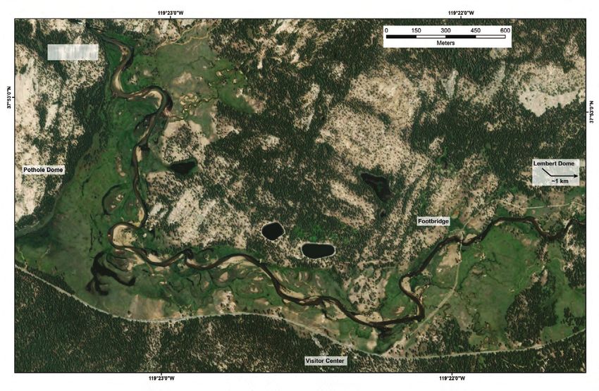
Figure 2. Maps of Tuolumne
Bedrock channel
Meadows study area. Upper
0 500 1,000 1,500 FEET
at meadow outlet panel is satellite imagery of
the study area. Lower panel
37°53’ is topography rendered from
airborne laser swath mapping
data of the study area. Darker
colors indicate steeper slopes
Lembert Dome
Pothole Dome ~1 kilometer
Soda Springs
Footbridge
Flow
37°52’30”
120
Tuolumne Meadows
Visitor Center
0 200 400 600 METERS
Bedrock channel
0 500 1,000 1,500 FEET
at meadow outlet
37°53’
Lembert Dome
Pothole Dome ~1 kilometer
Soda Springs
Footbridge
Flow
37°52’30”
120
Tuolumne Meadows
Visitor Center
Base imagery in upper panel from ESRI/Digital Globe. Imagery in lower
panel is a slopeshade/hillshade blend made from bare-earth elevation
data derived from the 2006 airborne laser swath mapping (ALSM).
tens of centimeters vertically from the low-water surface
elevation but are vegetated higher. The large flat expanse
Methods
of Tuolumne Meadows is a mosaic of older stream channel
forms, positioned 1–1.4 m above the low-water elevation. Field Surveys
Runoff is mostly generated annually during snowmelt,
though rainstorms do generate runoff that can lead to sudden The channel, streambanks, and meadow in Tuolumne
river level changes. Winter flooding is rare owing to cold Meadows were characterized using three-dimensional terrestrial
temperatures and snow accumulation, and summer flood laser scanning (TLS), this is also known as lidar (light detection
events are very rare, though spring runoff can be delayed until and ranging). Three TLS surveys were completed in September
June during cold years.
men20-7436_fig02 of each year 2016–2018 (table 1). The 2016 survey covered theMethods 5
Tuolumne River from the edge of dense trees just upstream from resistant rock) that defines the downstream end of the meadow
the Soda Springs footbridge (fig. 2) downstream to the prominent (Bedrock channel at meadow outlet in fig. 2). Figure 3 provides
bend to the north in the southwestern part of the meadow. The the location of the scan positions for each year displayed over
2017 and 2018 surveys covered the Tuolumne River from the edge a blend of slopeshade (slope map in which steeper slopes are
of dense trees just upstream from the Soda Springs footbridge portrayed with darker colors) and hillshade (terrain shaded by
downstream to just above the bedrock channel knickpoint (a artificial illumination) maps made from the bare-earth digital
distinct step in the river channel that forms a waterfall, caused by elevation model (DEM) for each year.
Table 1. Lidar point cloud data used in this study.
[Initial error estimates are observed errors in the accuracy of the point cloud georeferencing. ALSM, airborne laser swath mapping; TLS, terrestrial laser
scanning; m, meter; km2, square kilometers]
Number of Initial error
Survey dates Instrument Area (km2) Number of points
ground points estimate (m)
September 18–22, 20061 Optech 1233 ALTM (ALSM) ~7.9 24,339,975 6,537,774 0.15
September 20–25, 20162 Riegl VZ400 (TLS) ~1.4 479,877,894 147,223,346 0.02
September 11–15, 20172 Riegl VZ400i (TLS) ~1.92 513,428,999 149,367,512 0.02
September 11–14, 20182 Riegl VZ400i (TLS) ~2.1 754,557,695 233,124,284 0.05
1
Data collected by the National Center for Airborne Laser Mapping (NCALM) on behalf of the National Park Service (Stock, 2010).
2
Data collected for this study.
119°23’ 119°22’30” 119°22’ 119°21’30” 119°23’ 119°22’30” 119°22’ 119°21’30”
2016 2017
0 250 500 750 1,000 METERS
0 1,000 2,000 3,000 FEET
Bedrock channel
at meadow outlet
37°53’
Soda Spring
Footbridge
Soda Spring
Footbridge
Flow Flow
37°52’30”
2018 Bedrock channel
at meadow outlet
37°53’
Soda Spring
Footbridge
Flow
37°52’30”
Figure 3. Slopeshade maps made from terrestrial laser scanner
data of the study area from 2016–2018. Black dots indicate positions of
individual scans. Darker colors indicate steeper slopes. Backgrounds
are bare-earth slopeshade maps made from resulting point clouds.6 Streambank Erosion and Related Geomorphic Change in Tuolumne Meadows, Yosemite National Park, California
The basic principles of the survey methods employed were ground), medium vegetation (0.05–2.0 m above ground),
to collect laser scans in several positions in the meadow and along high vegetation (2.0–100 m above ground), and noise.
the Tuolumne River, merge these individual three-dimensional Because the streambanks along the Tuolumne River are
(3D) “point clouds” of XYZ coordinates and associated attribute commonly vertical to overhanging, the classification procedure
data into a single aligned 3D point cloud and use high accuracy of Pack and others (2012) was modified and implemented:
global positioning system (GPS) surveys to georeference the point clouds were tilted 50 degrees in 8 directions, ground
survey data into a common coordinate system. Care was taken classification was performed in each tilted position, then
to relocate scan positions each year, so that topographic and point clouds were rotated back to their original position and
vegetation occlusions were consistent, minimizing spurious recombined. All ground points within about 5–10 m of the
change-detection errors. Survey coverage expanded farther river channel edges were integrated into the final ground class,
downstream along the river channel and farther out into the and all duplicate points were removed, retaining ground points
meadow each year from 2016 to 2018. The resulting point clouds when ground and non-ground points were co-located during the
were filtered, classified, and gridded into derivative datasets used classification procedure.
for the analyses presented in this report.
Specifically, in 2016 data were collected from 62 scan
positions using a Riegl VZ400 laser scanner connected to a Leica Airborne Lidar Data
Viva GS15 real-time kinematic GPS receiver. In 2017, data were
collected from 98 scan positions using a Riegl VZ400i laser The ALSM data collected in September 2006 over
Tuolumne Meadows (Stock, 2012) were downloaded and
scanner connected to a Leica Viva GS15 real-time kinematic
transformed to the same coordinate system as the TLS
GPS receiver. In 2018, data were collected from 160 scan
(NAD83(2011)) UTM zone 11 north with WGS84 ellipsoid
positions using a Riegl VZ400i laser scanner connected in real
heights. They were reclassified using Terrascan software to
time to a Trimble R10 real-time kinematic GPS receiver. During
better characterize vegetation structure but without the use of
each survey, several retroreflective targets set up on stable and
the tilting algorithm used for the TLS because ALSM does not
carefully surveyed monuments were included to refine the final
resolve small overhanging streambanks.
georeferencing. The Riegl VZ400 and VZ400i scanners differ in
their speed, range, and types of orientation sensors. However, the
data from these two scanners are quite similar, and all three TLS Generation of Derivative Products from Lidar
surveys were postprocessed using similar workflows: individual
laser scans were oriented using an onboard electronic compass and Point Clouds
inclinometer and georeferenced using the GPS survey data. Errors
The classified point clouds were gridded to create
in orientation, location, and pitch were corrected using an iterative
derivative products that included bare-earth and full-feature
closest-point approach to minimize errors in overlapping areas
digital elevation models (DEMs), slope maps, and shaded relief
between individual point clouds, as implemented in Riegl RiScan
maps. The data are available in DeLong and Pickering (2020).
Pro software. These merged and aligned lidar point clouds had
From these products, canopy-height models (fig. 4) and grids
the final georeferencing refined using the surveyed targets. Errors
of vegetation most likely to be short meadow vegetation and
in the accuracy of the point cloud georeferencing are estimated
streambank willows were developed (fig. 5). Willow locations
at less than 2 cm for 2016 and 2017 and 5 cm for 2018, when
were characterized by identifying locations in which the
georeferencing errors were slightly higher for unknown reasons.
vegetation canopy was between 1 and 4 m above ground. Most
These are reported as “initial error estimates” in table 1. Additional
forest vegetation has canopy heights much taller than 4 m. This
empirical error analysis is presented below and allows for more
method does allow for non-willow vegetation between 1 and
realistic estimation of the level of detection (LoD) of elevation
4 meters tall to be mischaracterized as willows, but because
change using these data. These empirical error analyses use stable
of the interest in riverside vegetation for erosion control,
landscape features and indicate these initial georeferencing error
this may not be an important distinction from a geomorphic
estimates are conservative. The same GPS data were used for all
perspective. Vegetation with heights between 25 cm and 1 m
years for the monuments used for final georeferencing.
were mapped from the TLS data to provide an indication of
short meadow vegetation cover. It should be noted that TLS is
Point Cloud Processing limited in its ability to properly quantify short, dense vegetation
because at longer distances and low angles from the scanner,
The merged, georeferenced point clouds were filtered dense vegetation obscures the soil surface, resulting in short
for error points and reflections off water surfaces and were vegetation being classified as ground. This also leads to noise in
simplified using an octree approach that resulted in a point bare-earth change detection across the flat meadow regions as
density no greater than one point for each 2.5-cm-sized cube vegetation and scan views change from year to year. The ALSM
using Riegl RiScan Pro software. These cleaned point clouds data are quite noisy within 0.5 m or so of the ground surface
were classified into the following classes using Terrascan owing to flight line overlap and sensor accuracy issues typical
software (documentation available at Terrasolid.com, accessed of data from technology at that time (2006), and are therefore
December 12, 2019): ground, short vegetation (0–0.05 m above less effective at mapping short vegetation.Methods 7
A. 2006 Airborne laser swath mapping (ALSM)
119°23’ 119°22’30” 119°22’
EXPLANATION
Canopy height, in meters8 Streambank Erosion and Related Geomorphic Change in Tuolumne Meadows, Yosemite National Park, California
119°23’30” 119°23’ 119°22’30” 119°22’
EXPLANATION
Canopy height, in meters
0.25 to 1—Short vegetation
37°53’ 1 to 4—Mostly willows
37°52’30”
0 200 400 600 800 METERS
0 500 1,000 1,500 2,000 FEET
Universal Transverse Mercator, zone 11 North; North American Datum of 1983
Figure 5. Map of streambank willows and short vegetation along Tuolumne River derived from 2018 terrestrial
laser scanning (TLS) point clouds. Vegetation less than 1 m tall consists of a wide variety of meadow vegetation and
possibly some young willows. Some young conifers are included in the willow mapping. In general, vegetation close
to the stream channels is willows, and vegetation farther away is more likely to be conifers.
DEMs were generated from the point clouds using Golden results: the 50-cm grids appear the most spatially complete,
Software’s Surfer software. These were produced at 50-cm but tend to have errors in locations in which data have been
resolution with an inverse distance weighted mean algorithm interpolated over longer distances, whereas the 10-cm data can
with a 4-m search radius, and at 10-cm resolution with an inverse be considered higher accuracy but with data gaps in locations in
distance weighted mean algorithm with a 30-cm search radius. which no data exists within 30 cm.
The 50-cm DEMs are more spatially complete because data gaps Water and objects below water were not imaged by the laser
up to 4 m are interpolated. The 10-cm DEMs are less complete but scanners. Because of this, there are locations of no data in the
are a more accurate representation of the input point cloud. The change-detection results if an area that was ground one year then
two resolutions of DEMs provide different results when used for was water the next year owing to either changing water levels
elevation change mapping. or lateral stream migration, so some real geomorphic change
was missed when other data are compared to that collected in
the somewhat higher water level of 2017. Stream discharge
Landscape Change Mapping (as indicated by streamflow data are available at: https://irma.
nps.gov/AQWebPortal/Data/Location/Summary/Location/
To characterize streambank erosion, point- and channel- SIEN_YOSE_TUOLTIRO/Interval/Latest, accessed April 24,
bar deposition, and other topographic change, bare-earth DEMs 2020) was about 0.8 m3/s during the 2006, 2016, and 2018
generated from different years’ data were subtracted from one surveys. During the 2017 survey, discharge ranged from about 1
another, generating DEMs of difference (DoDs) (for example, to 5 m3/s, which led to several centimeters or more of difference
Wheaton and others, 2010). Comparisons with the 2006 airborne in water surface elevation between that survey and the others.
data (ALSM to TLS) were done at a grid resolution of 50 cm, and Procedures that would create a flat elevation surface across gaps
comparisons between TLS datasets were done at both 10- and created by presence of water were not implemented as they would
50-cm grid resolution. This provides different change-detection unfavorably affect topographic comparisons.
men20-7436_fig05Methods 9
Streambank Mapping volumetric estimates of landscape change. These levels were 0, 2,
and 10 cm for comparisons between TLS datasets, and 0, 4, and
Streambank locations in each dataset were manually digitized 10 cm for comparisons involving the 2006 ALSM data. These
to properly quantify streambank erosion. Lines were digitized as LoDs were implemented when gridded values of elevation change
close to the junction of the flat meadow surface and the sloped or were integrated into volumetric estimates, such that only DoD
vertical streambank as possible. These lines provided the clearest pixel values exceeding these values were used. Error estimates and
indication of stream bank dynamics in Tuolumne Meadows. LoDs are discussed in more detail later in this report.
Streambank positions were mapped as either “steep/active” or Though manual mapping of streambank locations from
“indistinct/stable” (fig. 6). Any streambank can become active in TLS and ALSM is the most accurate way to characterize
a large flood or stabilized if sediment deposition leads to channel streambank migration, other landscape changes such as
migration. For this study, the “steep/active” streambanks are deposition on channel and point bars is best characterized
mapped at high accuracy owing to their very distinct crest, and by the DoDs. However, dense vegetation and changes in
they tend to sit directly adjacent to the active channel, whereas vegetation annually can lead to errors in estimated elevation
those mapped as “indistinct/stable” are less accurate owing to their of true ground elevations. These errors in the bare-earth
less defined morphology and subjective locations. “Indistinct/ DEMs can then propagate into the change mapping, so
stable” streambanks are often found at point bar locations on the caution is required when interpreting DoDs. This is especially
inside bends of curves in the channel. The horizontal accuracy of apparent in low-relief areas relatively far from the scanner
mapped “steep/active” streambanks in 2016–2018 is estimated at locations and in areas of thick grass that obscures the ground
about 30 cm, and those mapped from the 2006 ALSM data have when viewed at a low angle. Occlusions caused by objects
accuracy estimated at about 1 m owing to the coarser resolution that block the laser instrument from surveying parts of the
base data. Most error comes from interpretation of ambiguities in landscape can also lead to spurious landscape change in areas
streambank locations where they do not form a sharp slope break scanned in detail from one survey but not the next. This issue
in the landscape. was mitigated by reoccupying the same scan positions each
To characterize erosion and deposition, the gridded elevation year. However, new survey positions were also added each
data were subtracted from one another to create DoDs at both 10- year to expand the survey footprint and to increase density of
and 50-cm resolution. These DoDs only have values at locations survey data.
which both input DEMs have pixel values, so a data gap in either The two metrics computed to characterize landscape change
DEM leads to a “no data” hole in the resulting DoD. These are rate of streambank migration (that is horizontal change)
DoDs were interpreted with varying levels of detection (LoD) from mapping, and volumetric change. Rate of streambank
of elevation change that minimize errors from propagating into migration was calculated as the average distance a streambank
119°23’ 119°22’30” 119°22’
EXPLANATION
2018 streambanks
Indistinct/stable
Steep/active Figure 6. Map of indistinct/stable
37°53’ and steep/active areas along
the Tuolumne River. Analyses of
landscape change from DoDs and
streambank mapping.
37°52’30”
0 200 400 600 800 METERS
0 500 1,000 1,500 2,000 FEET
Base image is a slopeshade/hillshade blend made from the 2018 lidar data.
Universal Transverse Mercator, zone 11 North; North American Datum of 198310 Streambank Erosion and Related Geomorphic Change in Tuolumne Meadows, Yosemite National Park, California
migrated along the length of streambank that changed. Volumetric elevation change. DoD values were extracted from areas judged
change was calculated in two ways. The first approach was to most likely to be geomorphically stable and unvegetated over
multiply average streambank retreat distances by the streambank the survey intervals. These areas include the paved California
height during the 2018 low-water conditions. This approach Highway 120, gravel and dirt park service roads, gravel hiking
overestimates the volume of sediment removed because some trails, and bedrock outcrops. Before calculating statistics, we
material is transiently preserved as slump blocks and sloped removed a very small amount of values of elevation change
material below the streambank even where the streambank has greater than 30 cm from these areas because these were either real
retreated. This material is likely removed in subsequent years geomorphic change that should not be used as stable areas for
when floods act upon the slumped blocks at the channel margin. error analysis, isolated objects present in only one scan, or changes
Thus, the multiyear streambank retreat rate is proportional to the in vegetation. Table 2 presents these results. They indicate that
volumetric change rate, but with varying lag times owing to the comparisons between TLS data can be done using a LoD of about
time needed to remove transient slump-block material. 0.1–1 cm, and comparisons involving ALSM data can be done
The second approach was to take a direct measurement of using a LoD of about 2–4 cm. The average DoD value extracted
volumetric change from the DoD and apply it to streambanks as from these areas is an indication of LoD in change mapping, and
well as point and channel bars. For this, elevation changes were the standard deviation is best thought of as the amplitude of noise
extracted at all locations where the DoD has data within specified in the datasets caused by changing microtopography, variability
areas. These areas include zones of erosion, zones of deposition, in location of individual XYZ points within grid cells leading to
and the entire channel system. These data are less accurate averaging differences, and other scatter in the data, rather than a
when the relatively high-water 2017 survey was used because formal error metric. No specific evidence or knowledge exists of
some pixels in 2017 were obscured by water covering sediment any road or trail grading occurring between surveys that would
and were therefore not accounted for in the DoDs. In general, have affected these data. For results displayed in tables and
volumetric change calculated from 2006 or 2016 to 2017 will be discussed in this report, the LoD used for data derived from TLS
an underestimate of true volumetric change. Elevation differences to TLS comparisons was 2 cm, and comparisons of TLS with
measured from 2006 to 2016 or 2018 and 2016 to 2018 should ALSM data were performed with a LoD of 4 cm.
be more accurate representations of volumetric change because
of similar water levels during those years. However, the true
volumetric change at eroding streambanks is in between the two
methods used here, and the horizontal displacement of streambank
Results
position is the most reliable indication of streambank migration. The three terrestrial laser scan surveys were used to
Analyses were conducted and results presented for each generate the derived topographic data products available in
erosion zone and include net erosion and deposition for a DeLong and Pickering (2020). In the following sections,
streambank and any channel or point bars adjacent to or directly vegetation mapping, streambank mapping, and landscape
across the channel from the streambank. This is not because change analyses are presented.
sediment erosion and deposition are tightly coupled in a single
location; generally eroded material from a streambank will
be transported downstream rather than be deposited locally. Vegetation Mapping
However, because of interest in the stability of cross-sectional
geometry and to provide data comparable to typical cross- The three-dimensional point clouds contain information
section-based monitoring efforts, the dynamics of landscape about not only the ground surface, but also all vegetation and
change across the stream valley at locations of migrating objects above the ground. By gridding the elevation of points at
streambanks may be of interest. the top of vegetation to generate “full featured” DEMs as well as
The TLS surveys were performed during the late-summer those on the ground to generate bare-earth DEMs and subtracting
low-water conditions. The measured landscape change occurred the two models, vegetation canopy height can be characterized
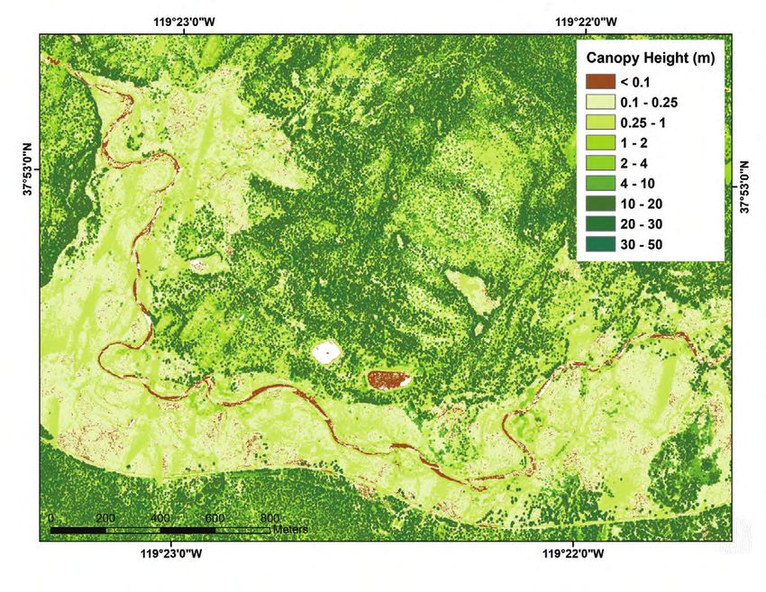
mostly in the spring and (or) early summer of that year, (fig. 4). These canopy maps indicate the contrast between the
primarily during snowmelt-caused peak river discharge, or as a conifer forest (darker green) on the slopes adjacent to the meadow
result of rain events which happen occasionally throughout the and the generally short vegetation (brown to light green) in the
years. As such, when, for example, “erosion from 2016-2017” meadows. Along the stream channels, bare depositional bars are
is discussed, this erosion occurred mostly or totally in the spring common, and some riparian vegetation is present.
and summer of 2017. To more specifically characterize vegetation types, the stature
of meadow vegetation and riverside willows were considered. Tall
willows in Tuolumne Meadows include Salix orestera, lemmonii,
Empirical Error Estimate Refinement Using eastwoodiae, and planifolia (Sierra, Lemmon’s, mountain, and
Stable Landscape Areas diamondleaf willows, respectively), which have characteristic
heights up to about 4 m. Plants with heights up to 4 m, and
The development of the DoD change maps provides an meadow vegetation between 0.25 and 1 m tall were extracted from
opportunity to further extract indicators of accuracy and LoD of the point clouds to characterize willow and meadow vegetation.You can also read


