Study of the thermal and nonthermal emission components in M31: arXiv
←
→
Page content transcription
If your browser does not render page correctly, please read the page content below

Astronomy & Astrophysics manuscript no. AA                                                                                           ©ESO 2021
                                               May 24, 2021

                                               Study of the thermal and nonthermal emission components in M31:
                                                          the Sardinia Radio Telescope view at 6.6 GHz?
                                                    S. Fatigoni1, 2 , F. Radiconi1, 3 , E.S. Battistelli1, 3, 4 , M. Murgia4 , E. Carretti5 , P. Castangia4 , R. Concu4 , P. de
                                                   Bernardis1, 3 , J. Fritz6 , R. Genova-Santos7, 8 , F. Govoni4 , F. Guidi7, 8 , L. Lamagna1, 3 , S. Masi1, 3 , A. Melis4 , R.
                                               Paladini9 , F.M. Perez-Toledo8 , F. Piacentini1, 3 , S. Poppi4 , R. Rebolo7, 8 , J.A. Rubino-Martin7, 8 , G. Surcis4 , A. Tarchi4 ,
                                                                                                               V. Vacca4

                                                     1
                                                         Sapienza University of Rome, Physics Department, Piazzale Aldo Moro 5, 00185 Rome, Italy
arXiv:2105.10453v1 [astro-ph.GA] 21 May 2021

                                                     2
                                                         University of British Columbia, Department of Physics and Astronomy, Vancouver, BC, V6T 1Z1, Canada
                                                     3
                                                         INFN - Sezione di Roma, Piazzale Aldo Moro 5 - I-00185, Rome, Italy
                                                     4
                                                         INAF - Osservatorio Astronomico di Cagliari, Via della Scienza 5 - I-09047 Selargius (CA), Italy
                                                     5
                                                         INAF - Istituto di Radioastronomia - Via P. Gobetti, 101 - I-40129 Bologna, Italy
                                                     6
                                                         Instituto de Radioastronomia y Astrofisica, UNAM, Campus Morelia, A.P. 3-72, C.P. 58089, Mexico
                                                     7
                                                         Instituto de Astrofisica de Canarias, C/Via Lactea s/n, E-38205 La Laguna, Tenerife, Spain
                                                     8
                                                         Departamento de Astrofsica, Universidad de La Laguna (ULL), E-38206 La Laguna, Tenerife, Spain
                                                     9
                                                         Infrared Processing Analysis Center, California Institute of Technology, Pasadena, CA 91125, USA
                                                         e-mail:          sfatigoni@phas.ubc.ca, federico.radiconi@roma1.infn.it, elia.battistelli@roma1.infn.it,
                                                         matteo.murgia@inaf.it

                                                     Received 27 November 2020 / Accepted 20 April 2021

                                                                                                                  ABSTRACT

                                                     Context. The Andromeda galaxy is the best-known large galaxy besides our own Milky Way. Several images and studies exist at all
                                                     wavelengths from radio to hard X-ray. Nevertheless, only a few observations are available in the microwave range where its average
                                                     radio emission reaches the minimum.
                                                     Aims. In this paper, we want to study the radio morphology of the galaxy, decouple thermal from nonthermal emission, and extract
                                                     the star formation rate. We also aim to derive a complete catalog of radio sources for the mapped patch of sky.
                                                     Methods. We observed the Andromeda galaxy with the Sardinia Radio Telescope at 6.6 GHz with very high sensitivity and angular
                                                     resolution, and an unprecedented sky coverage.
                                                     Results. Using new 6.6 GHz data and Effelsberg radio telescope ancillary data, we confirm that, globally, the spectral index is ∼
                                                     0.7 − 0.8, while in the star forming regions it decreases to ∼ 0.5. By disentangling (gas) thermal and nonthermal emission, we find that
                                                     at 6.6 GHz, thermal emission follows the distribution of HII regions around the ring. Nonthermal emission within the ring appears
                                                     smoother and more uniform than thermal emission because of diffusion of the cosmic ray electrons away from their birthplaces.
                                                     This causes the magnetic fields to appear almost constant in intensity. Furthermore, we calculated a map of the star formation rate
                                                     based on the map of thermal emission. Integrating within a radius of Rmax = 15 kpc, we obtained a total star formation rate of
                                                     0.19 ± 0.01 M /yr in agreement with previous results in the literature. Finally, we correlated our radio data with infrared images of
                                                     the Andromeda galaxy. We find an unexpectedly high correlation between nonthermal and mid-infrared data in the central region,
                                                     with a correlation parameter r = 0.93. Finally, by computing the logarithmic 24µm /21cm ratio q24µm , we find a decreasing trend with
                                                     increasing galactocentric distance and an increasing dispersion. The logarithmic far-infrared-to-radio ratio is found to be 2.41 ± 0.04.
                                                     Key words. Galaxies: Individual: Messier 31; Radio continuum: galaxies, ISM; Radiation mechanisms: nonthermal, thermal

                                               1. Introduction                                                                The galaxy presents a large central bulge. The bulge is de-
                                                                                                                          fined as the central region that has an extension of 50 in the opti-
                                               The Andromeda galaxy (Messier 31, M31) is the largest galaxy               cal band, corresponding to a proper size of 1.1 kpc (Morton et al.
                                               of the Local Group, which includes the Milky Way, the Triangu-             1977). The bulge contains dilute ionized gas and a few dense star
                                               lum galaxy (M33), and several other smaller galaxies including             clusters. V- and I-band Hubble Space Telescope (HST) Planetary
                                               the satellite Messier 32 (M32) and Messier 110 (M110). Messier             Camera images show that the central region seems to have two
                                               31 is a large disk galaxy at a distance of 780 kpc from Earth              separate concentrations of light that are about 0.5" apart (Lauer
                                               (Stanek & Garnavich 1998), and has a proper redshift of z=-                et al. 1993). One of these probably contains a dense central ob-
                                               0.001 (de Vaucouleurs et al. 1991), where the negative value               ject, presumably a black hole of mass MBH ' 106 M , while the
                                               shows that it is moving towards the Milky Way.                             other might be a star cluster. There is a ring circling the bulge at
                                                                                                                          a radius of about 10 kpc, and most of the young disk stars lie in
                                                                                                                          this ring or just outside it (Haas et al. 1998; Gordon et al. 2006;
                                                ?
                                                    Table A.1 and the 6.6 GHz SRT map are available in electronic form    Ford et al. 2013). Going to greater distances from the center we
                                               at the CDS via anonymous ftp to cdsarc.u-strasbg.fr (130.79.128.5) or      find the HI (Braun et al. 2009) layer that flares out to become
                                               via http://cdsweb.u-strasbg.fr/cgi-bin/qcat?J/A+A/

                                                                                                                                                                     Article number, page 1 of 36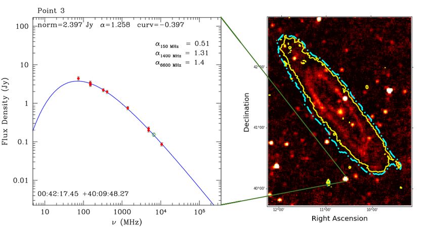
A&A proofs: manuscript no. AA

thicker. The M31 galaxy is the brightest of the Messier objects,        used three new deep radio surveys of M31 made with the Ef-
with an apparent magnitude (V) of 3.4 (Gil de Paz et al. 2007)          felsberg radio telescope at 2.645 GHz, 4.85 GHz, and 8.35 GHz
and an apparent extension of approximately 1 × 3 deg2 (Nilson           to perform a detailed study of the spectral index maps as well
1973) due to the high inclination with respect to the line of sight,    as thermal and nonthermal emission scale lengths. Beck et al.
which is assumed to be of 75° (Gordon et al. 2006) considering          (2020), using nine frequencies, found a total spectral index of
that 90° means an edge-on orientation.                                  0.71 ± 0.02 and a synchrotron spectral index of 0.81 ± 0.03; they
     Observations by the infrared Spitzer Space Telescope re-           also found that the synchrotron emission ring is wider than the
vealed that M31 contains about ' 1012 stars (Peñarrubia et al.          thermal emission one.
2014), which is at least twice the number of stars contained in             In Battistelli et al. (2019) we showed that the total integrated
the Milky Way, and the total mass of the galaxy is estimated to         emission at 6.6 GHz from M31, integrated over an elliptical re-
be M M31 = 1.5 × 10¹² M (Barmby et al. 2006). High-resolution           gion of 91.50 and 59.50 semi-axes, is at the level of 1.20 ± 0.06
(FWHM=9”) Westerbork Synthesis Radio Telescope (WSRT)                   Jy. Comparing different ancillary data allowed us to calculate
observations of the 21 cm line by Braun et al. (2009) were used         the emission budget; we found strong and highly significant ev-
to calculate the total neutral gas mass, which turned out to be in      idence for anomalous microwave emission (AME) at the level
the range 4.4 to 5.5 × 10⁹ M (Fritz et al. 2012). CO observa-           of 1.45+0.17
                                                                                −0.19 Jy at the peaking frequency of '25 GHz. By decom-
tions by Nieten et al. (2006) within a field of 0.5◦ × 1.8◦ led to an   posing the spectrum into known emission mechanisms, such as
estimate of the mass of molecular gas of the order of 2.63 × 10⁸        synchrotron, free-free, thermal dust, and AME, we found that
M (Fritz et al. 2012). While the former observations do not in-         the overall emission from M31, at frequencies below 10 GHz,
clude the whole galaxy disk, they most certainly encompass the          is dominated by synchrotron emission with a spectral index
majority of the molecular gas (about 95% of the total molecular         of 1.10+0.10
                                                                                −0.08 , with subdominant free-free emission. At frequen-
mass, according to Nieten et al. 2006).                                 cies of ∼10 GHz, AME has a similar intensity to that of syn-
     Because of its size and distance in the sky, M31 is an excel-      chrotron and free-free emission, overtaking these components at
lent laboratory with which to further study and perhaps confirm         frequencies between 20 GHz and 50 GHz, whereas thermal dust
the physical mechanisms and properties that have so far only            emission dominates the emission budget at frequencies above
been studied in detail in our own Galaxy. It also provides in-          60 GHz, as expected. For the purpose of this paper, we refer
formation about the general features of a typical disk galaxy.          to the free-free emission as thermal emission, and to the syn-
The M31 galaxy has been studied at several wavelengths: Fermi           chrotron emission as nonthermal emission, assuming any other
LAT was used to detect gamma-ray emission in the energy range           emission mechanism to be negligible at 6.6 GHz. K-band ob-
200 MeV - 20 GeV (Abdo et al. 2010). NuSTAR permitted the               servations with improved angular resolution (e.g., 0.90 with the
study of hard X-ray emission allowing X-ray binaries and neu-           Sardinia Radio Telescope at 22 GHz) will be key to disentan-
tron stars/black holes to be resolved (Wik et al. 2016). XMM,           gling AME models, and to studying AME over an entire galaxy
ROSAT, and CHANDRA were used to study its X-ray emis-                   outside of our own with high angular resolution (Battistelli et al.
sion (Stiele et al. 2010). Ultraviolet (UV) measurements were           (2012), Radiconi et al. in preparation).
used to study interstellar extinction (Clayton et al. 2015) as well         This paper is organized as follows. The characteristics of
as the circumgalactic medium, finding a very extended ionized           the observations, the scanning strategy, and the data analysis
medium which may overlap with a similar one originating from            pipeline of C-band data are described in Sect. 2. In Sect. 3 we
our Milky Way (Lehner et al. 2020). Optical and near-infrared           describe all the ancillary maps used in this paper and the recipes
(NIR) observations were used to investigate the stellar composi-        that were adopted to make their geometry and angular resolution
tion (Sick et al. 2014). The IR and submillimeter (submm) emis-         uniform. The removal of compact sources is presented in Sect. 4.
sion of M31 were studied by Fritz et al. (2012) and the HELGA           In the same section we also compare the normalized differential
collaboration. These latter authors used data obtained from the         count of compact sources with theoretical predictions. In Sect. 5
Herschel satellite to characterize the dust emission of M31, and        we carry out an analysis of the morphology of M31 by investi-
to construct maps of the dust surface density, the dust-to-gas ra-      gating the galaxy spectral index map. Thermal and nonthermal
tio, the starlight heating intensity, and the abundance of poly-        maps at 6.6 GHz are presented in Sect. 6, while in Sect. 7, start-
cyclic aromatic hydrocarbons (PAHs).                                    ing from the thermal map, we derive a map of the star formation
     The radio and microwave emission of M31 have been ob-              rate (SFR), and compare this to what was previously found in
served at high angular resolution (FWHM < 50 ) in the last three        the literature. In Sects. 8 and 9 we analyze the correlation be-
decades with the Effelsberg radio telescope (Beck et al. 2020;          tween radio-continuum and IR data, studying how thermal and
Berkhuijsen et al. 2003, 1983), the Westerbork Synthesis Radio          nonthermal emissions are related to IR emission. We also com-
Telescope (WSRT, Braun et al. 2009), and the Very Large Array           pute the parameter qFIR and compare the result with the expected
(VLA, Condon et al. 1998). Combined Effelsberg and VLA ob-              value. Finally, in Sect. 10 we summarize our results.
servations at 1.46 GHz and Effelsberg data at 4.85 GHz indicate a
global nonthermal spectral index of α s = 1.0 ± 0.1 (Berkhuijsen        2. Sardinia Radio Telescope observations of M31
et al. 2003), which is consistent with the value found by Bat-
tistelli et al. (2019), who studied the overall flux density emis-      2.1. Sardinia Radio Telescope
sion from radio to IR wavelengths. Berkhuijsen et al. (2003),           The Sardinia Radio Telescope (SRT 1 ) is an Italian facility for ra-
assuming a nonthermal spectral index equal to 1, derived (gas-)         dio astronomy run by the Istituto Nazionale di Astrofisica, INAF,
thermal and nonthermal maps at 4.85 GHz, finding that the ther-         which was formally inaugurated in 2013 after completion of
mal emission is stronger in the northern part of M31, whereas           technical commissioning (Bolli et al. 2015). The scientific com-
the nonthermal emission is nearly homogeneous over the whole            missioning of the telescope was carried out in the period 2012-
ring. This homogeneity suggests that recent star formation does         2015 (Murgia et al. 2016; Prandoni et al. 2017). At the begin-
not lead to a local increase in the number of relativistic electrons    ning of 2016 the first call for single-dish early science programs
and/or magnetic field strength. Strong thermal emission was also
                                                                        1
found within the central region of the galaxy. Beck et al. (2020)           http://www.srt.inaf.it/

Article number, page 2 of 36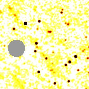
Fatigoni, Radiconi, Battistelli, Murgia et al.: M31 map at 6.6 GHz

(ESPs) was issued, and the observations started on February 1,             Telescope                        SRT (64m)
2016. The SRT observations of M31 at 6.6 GHz presented in this             Receiver                         C-band (5.7-7.7 GHz)
work are part of these ESPs. The SRT is placed 35 km north of              Backend                          SARDARA
Cagliari (Lat: 39° 29’34”N - Long: 9° 14’42”E) on the island of            Spectroscopy                     16384 channels
Sardinia at 600 m above sea level. The optical system is based             Backend bandwidth                1.5 GHz
on a quasi-Gregorian dish antenna, with a primary mirror of 64             Channel spacing                  91.6 kHz
m in diameter, and a secondary mirror of 9 m, which is shaped              Observed frequency range         6.0-7.25 MHz
in such a way as to minimize the standing wave bouncing be-                Beam size                        2.90 @ 6.6 GHz
tween the two reflectors. Three additional mirrors increase the            Polarization                     Full Stokes
number of focal positions. A key feature of the SRT is its active          Scanning strategy                Orthogonal raster subscans
surface, composed of a total of 1116 electromechanical actuators           Scanning speed                   60 /s
able to correct deformations induced by gravity on the primary             Sample rate                      25 spectra/s
surface. The SRT has an angular resolution of 2.90 (FWHM) at a             < T sys >                        37 K
frequency of 6.6 GHz.                                                      Map size                         2.4 deg × 3.1 deg ' 7.4 deg2
    The suite of backends currently available on site includes             Total number of scans            22 RA + 22 Dec
SARDARA (SArdinia Roach2-based Digital Architecture for                    Total observation time           64h
Radio Astronomy; Melis et al. 2018). The SARDARA back-                     Reached sensitivity              0.43 mJy/beam
end is a wide-band digital backend based on ROACH22 tech-                Table 1. Main characteristics of the C-band SRT observations on M31.
nology, and can divide the signal in the given bandwidth into up
to 16384 channels for spectropolarimetric observations. We used
this backend for our observations.
                                                                         RA subscans and 161 Dec subscans. Table 1 reports the main de-
                                                                         tails of the observations.
2.2. C-band observation                                                       Before starting the observations, a set of daily preliminary
                                                                         operations were performed. These include the configuration of
The main goal of the observations presented in this paper is to          the backend, setting of the amplifier attenuation factors (to en-
map the whole M31 galaxy in the C-Band down to a sensitiv-               sure linearity), secondary mirror positioning (by focusing a
ity of 0.4 mJy/beam in order to create a high-sensitivity/high-          bright radio source), and spectroscopic system acquisition and
angular-resolution map of M31 microwave emission covering its            pointing checks. The calibrators were observed during each ses-
full extension, limited by the confusion noise at this frequency         sion, when M31 was over the antenna critical elevation of 85 deg,
and angular resolution (Bondi et al. 2003; Condon 1974). We set          the SRT being equipped with an Alt-azimuthal mount. The ob-
the Local Oscillator at 5.9 GHz and we use the SARDARA con-              servations were completed in 64 h, divided in 6 days, during
figuration with 1.5 GHz bandwidth sampled with 16384 chan-               which we carried out 22 complete scans of the galaxy.
nels of 91.6 kHz in width. The data cube will be analyzed in
greater detail in a search for spectral line emission from vari-
ous transitions (Tarchi et al., in prep.). We set the Focus Selector     2.3. Data acquisition
filter to select the frequency range from 6.0 to 7.2 GHz, which
                                                                         Once collected, the data were analyzed using the Single-dish
defines our observing bandwidth. The central frequency of our
                                                                         Spectral-polarimetry Software (SCUBE, see Murgia et al. 2016),
observations is therefore 6.6 GHz. Traditionally, C-band is cen-
                                                                         which was created specifically for treating data acquired with the
tered at about 5 GHz, while the band around 6.6 GHz is known
                                                                         SRT. SCUBE is a package dedicated to the reduction and anal-
as the C-high band. For simplicity, in this paper we refer to the
                                                                         ysis of single-dish data and its combination with interferometric
6.6 GHz data as C-band data.
                                                                         observations. SCUBE is written in C++ and is developed and
     We decided to cover the galaxy with a rectangle of 7.4 deg2         maintained by M. Murgia and F. Govoni; it allowed us to im-
centered at (RA; Dec) = (0h 42m 48s; +41◦ 160 4800 ). To the             port the data, extract, analyze, and flag the spectra, do the base-
best of our knowledge, this is the biggest map ever produced at          line subtraction, perform calibration, and generate the final maps
this frequency and angular resolution with a single-dish radio           with different methods.
telescope.                                                                   As a first step in the data reduction process we removed
     The map size was determined by the minimum contour that             the backend "birdies" (dead channels occurring in SARDARA
includes the galaxy, to which we added a Map Edge of 0.25 deg            data) and the well-known persistent radio-frequency interfer-
in each of the two scanning directions. The minimum contour              ence (RFI) that affect specific spectral windows at the SRT.
was estimated by comparing the two maps provided by Her-                 These omnipresent signals were removed a priori by applying
schel/SPIRE at 250 µm (Fritz et al. 2012) and Planck at 857 GHz          the same flag table to all observing days. All the remaining spo-
(Planck Collaboration et al. 2014); which are supposed to trace          radic RFI signals (e.g. satellites or other transient ambience dis-
the galaxy in its maximum extension. Planck and Herchel 5σ               turbances) were removed later in the analysis with automated
contours are presented in the right panel of Fig. 3. The aim of          flagging methods. Overall, the amount of data erased due to RFI
adding an extra padding is to have a sky region that is completely       accounts for about 30% of the total.
free from M31 emission and that we can use to estimate the                   The baseline subtraction was carried out differently for the
background and decouple this from the signal coming from the             calibrators and for the M31 scans. To estimate the baseline for
galaxy. We adopted an on-the-fly map-scanning strategy, which            calibrators we made a linear fit over 10% at the beginning and at
means orthogonal subscans along right ascension (RA) and dec-            the end of each subscan, and then removed this linear trend from
lination (Dec) spaced by 54 arcsec (FWHM/3). We used a scan-             the data.
ning speed of 60 /s. Covering the 7.4 deg2 of our map required 209           To create a baseline model for the M31 scans we used a mask
                                                                         to cover the part of the map that we knew could possibly con-
2
    https://casper.ssl.berkeley.edu/wiki/ROACH2                          tain either galactic emission from M31 itself or any bright back-
                                                                                                                   Article number, page 3 of 36
A&A proofs: manuscript no. AA

ground point source. The remaining part of the field of view was    2.6. Map making
considered as "cold sky" and was used to perform a linear fit to
the baseline subscan by subscan (see Sect. 2.5).                    In the creation of our final total intensity map, we combined the
                                                                    scans by taking an average of all of them in order to increase
                                                                    the signal-to-noise ratio. A direct stacking would be heavily af-
2.4. Calibration                                                    fected by the scanning noise present in the individual on-the-fly
                                                                    maps, which takes the form of the typical pattern of "stripes"
Data calibration included bandpass and flux density calibration.    oriented along the scanning direction. These stripes can be due
These were carried out at the beginning of the map extraction       to imperfect RFI removal or short-term fluctuations in the at-
process and performed channel by channel. The bandpass cali-        mosphere or in the receiver gain. Sometimes these features are
bration was necessary to set the instrument responsivity for ev-    not totally removed during the flagging and the baseline subtrac-
ery channel. For this purpose we used specific calibrators, like    tion process, and so they persist in the final map. These features
J0542+4951 (3C147), with stable and known spectra.                  are easier to identify if we analyze the map in the perpendicular
    We applied the gain-elevation curve correction to account for   direction with respect to the direction of the corrupted subscan
the gain variation with elevation due to the gravitational stress   (Emerson & Graeve 1988). To this purpose, SCUBE implements
changes in the telescope structure. We do not compensate for the    both Fourier and wavelet map-making methods. In the Fourier
atmosphere opacity however, considering that the correction is      transform plane, the scanning noise terms from any single scan
negligible at these frequencies.                                    appear only on a narrow band passing through the origin, with a
    The counts-to-Jansky conversion factor was derived by           width inversely proportional to the characteristic scale lengths of
means of a two-dimensional Gaussian fit to the Stokes L             the baseline drifts in the original scan. The final map is created
and R images of the standard flux density calibrators 3C147,        by incorporating a second scan in an orthogonal direction so that
J0137+3309 (3C48), J1331+3030 (3C286), and J1411+5212               once the second scan is also transformed in the Fourier plane,
(3C295). We adopted the flux density scale of Perley & Butler       the second map only intersects the error terms of the first map
(2013). The systematic uncertainty is assumed to be 5% of the       at the origin. The knowledge of the approximate scale length of
calibrator flux density.                                            the baseline drift of each map, and so the width of each band
    All calibrator observations were made during the interrup-      error in the Fourier plane, enables an optimally weighted com-
tion of the M31 scans when the galaxy was too highly elevated       bination of Fourier terms of each data set to be made (Emerson
on the sky or at the end of the scans. Data were acquired during    & Graeve 1988). In the wavelet space, the logic is the same, ex-
four cross scans on each of the calibration sources. The cross      cept that the unwanted scanning noise is isolated and filtered out
scans were made at a velocity of 10 /s and each subscan was 200     using a convenient merging of the stationary wavelet transform
long.                                                               (SWT) coefficients (Murgia et al. 2016). One advantage of the
                                                                    SWT method compared to the Fourier method is that there is no
                                                                    need to determine an optimal width for the weights of the noise
2.5. Baseline subtraction                                           bands. While the noise bands partially overlap at the center of
                                                                    the Fourier plane, they are completely separated in the wavelet
Before stacking the subscans to form the maps, we performed a       domain. Indeed, the horizontal and vertical detail coefficients of
subscan baseline removal in order to set all the emission coming    the two orthogonal scans can be opportunely mixed while the di-
from blank fields to zero. To this purpose we applied a mask.       agonal detail coefficients and the approximation coefficients are
Our mask map was created starting from three different maps         averaged.
of the M31 region: the NRAO VLA Sky Survey (NVSS) map                    We verified that both the Fourier and SWT de-stripping tech-
at 1.4 GHz (Condon et al. 1998) which contains point sources,       niques give consistent results. However, we noted that the SWT
the Spitzer MIPS map at 12.5 THz (Gordon et al. 2006), and          performed slightly better than the Fourier method and therefore
the Planck 850 GHz map (Planck Collaboration et al. 2020) that      we opted the former.
traces the extension of the galaxy with thermal dust emission. We
renormalized and combined the set of maps creating a mask from           As a last step in the map-making process we corrected the
which the baseline is calculated. The mask, combined with the       final map for the residual base level. To this purpose, we masked
0.25 deg MapEdge, was finally used to estimate the background       the emission from M31 and applied the Papoulis-Gerchberg Al-
level by fitting a linear model to the emission in the nonmasked    gorithm (PGA, Papoulis 1975) to model and interpolate the sur-
region.                                                             rounding base level over the excluded data. SCUBE provides an
                                                                    application of the PGA that allows the user to reconstruct the
    At this point, in order to generate the final map, we per-      missing part of an image by imposing a low pass filter in the
formed a new flagging of the data to remove isolated spikes         spectral domain. The signal extrapolation is carried out by iterat-
or short-time RFIs in an automated fashion. Following this ap-      ing alternately between time (spatial) and spectral domains until
proach, we were able to flag all the data that deviate by more      convergence is reached. To this end, we masked out an ellipti-
than 3σ, where σ is a combination between the single subscan        cal region of 910 .5 and 590 .5 semi-major and semi-minor axis,
rms and the sky model noise according to:                           respectively (PA=-52deg), centered on the innermost regions,
                                                                    and we reconstructed the missing signal by imposing that the
                                                                    reconstructed map retains no power below a spatial scale corre-

σ2 = rms2sub−scan + (mod_errsys · model)2 .                   (1)
                                                                    sponding to the ellipse major axis. This is achieved by a con-
                                                                    volution with a Gaussian tapering in the spectral domain. The
The parameter mod_errsys was chosen to be 0.5. This method          reconstructed base-level image is then subtracted from the final
was iterated until convergence was reached: three iterations for    map, which allows the removal of residual large-scale features
each set of data were needed. At this point, it was possible to     left over after baseline removal and map-making, and large-scale
create a new set of images where, as expected, the rms level was    features in foreground and background emission, bringing the
lower with respect to the previous images.                          map back to a zero-level outside the galaxy, as already shown in
Article number, page 4 of 36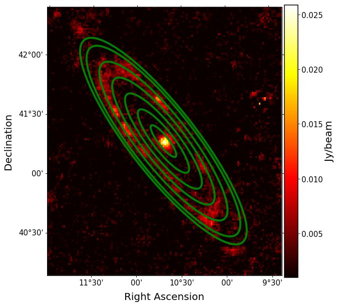
Fatigoni, Radiconi, Battistelli, Murgia et al.: M31 map at 6.6 GHz

Battistelli et al. (2019). Figure 1 shows our final map of M31 at      3.3. Ancillary data treatment
6.6 GHz.
                                                                       Each one of the aforementioned maps is characterized by a given
                                                                       angular resolution and geometry (i.e., pixelization on the sky). In
2.7. Map statistics                                                    order to compare different maps, it was necessary to bring all of
                                                                       them to the same coordinate system and angular resolution.
In order to provide an estimate of the sensitivity level reached in        We used the Montage 6.0 software6 to modify the coordinate
our map, we masked the emission from point-like radio sources.         system of the maps and convert it to the SRT C-band pixeliza-
Details on how compact sources are removed from the map are            tion. Once all the maps were in the same World Coordinate Sys-
reported in Sect. 4. In our source-subtracted map, considering         tem (WCS, Mink 1997) reference frame, they were convolved to
our pixel size of 0.90 , and the SRT beam in the C-band, we            the same angular resolution.
derived the rms fluctuations from two 0.4 deg2 uncontaminated              Depending on the purpose, three different final angular reso-
regions. We repeated the same analysis on the SWT map be-              lutions were used: 140 , 5.00 , and 30 .
fore and after applying the flagging. We found consistent (al-
though slightly different) results in the two maps: we obtained             – For the sole purpose of estimating the qFIR parameter, the
a rms mean value of 0.44 mJy/beam before flagging and 0.43                    Herschel 100 µm map and the IRAS 60 µm map were con-
mJy/beam after flagging. Therefore, from this first analysis, we              volved to the common resolution of 140 .
have a final value for the rms of 0.43 mJy/beam. This value is              – Convolution of all the maps to the resolution of the Effels-
fully compatible with the expected value from confusion noise,                berg 2.7 GHz map (5.00 ) was carried out to disentangle ther-
assuming a spectral index of 0.7: con f noise = 0.44 mJy/beam                 mal and nonthermal emission (see Sect. 6) and to correlate
(Condon 1974).                                                                these two emission mechanisms to IR data (see Sect. 8).
                                                                            – We convolved the two Spitzer maps, the 1.4 GHz Effelsberg,
                                                                              and our SRT C-band image to 30 to extract a spectral index
3. Ancillary data                                                             map (see Sect. 5).

In this section we describe the ancillary maps used throughout
this work. The ancillary maps are described in two different sec-      4. Compact sources
tions, one relative to radio and microwave wavelengths and the         A large number of sources can be seen in the 2.4 × 3.1 deg2
other to IR observations.                                              C-band map shown in the left panel of Fig. 1. In order to cal-
                                                                       culate a proper estimate of the intrinsic brightness of M31, it
3.1. Radio data                                                        is necessary to identify and remove all the signals coming from
                                                                       these sources. To this end, we generated a point-source catalog of
For radio wavelengths, we used three maps acquired with                M31 at 6.6 GHz. Aside from point-source subtraction, we used
the Effelsberg Radio Telescope3,4 , at 1.46 GHz, 2.7 GHz, and          this catalog to verify the theoretical prediction on the number of
4.85 GHz. With its 100-metre primary mirror diameter, Effels-          sources we expect to find with a certain flux density in a given
berg reaches an angular resolution of 5.00 (Beck & Grave 1982)         area, according to a specific model.
and 2.80 (Berkhuijsen et al. 2003) at 2.7 GHz and 4.85 GHz, re-            We started by extracting a point-source catalog from the
spectively. The 1.46 GHz map angular resolution of 0.750 (Beck         NRAO VLA Sky Survey at 1.4 GHz (Condon et al. 1998) which
et al. 1998) was achieved combining Effelsberg data with VLA           has an angular resolution of 4500 and a rms of 0.5 mJy/beam.
data. Moreover, we used the SRT map at 1.385 GHz (Melis et al.         We relied on the relatively high angular resolution and sensitiv-
2018), with an angular resolution of 13.90 , to correlate radio and    ity of the NVSS to obtain a good prior for the coordinates of
IR data.                                                               the points sources in the direction of the M31 field. This is par-
                                                                       ticularly helpful in the subtraction of those point sources seen in
                                                                       projection against (or embedded in) the extended emission of the
3.2. Infrared data                                                     galaxy, as we show in Figure 2 where the SRT C-band contours
                                                                       are added to the NVSS image. Indeed, the finer NVSS resolution
Infrared data were used to characterize stellar and dust emis-
                                                                       also allowed us to resolve nearby sources not easily discernible
sion and explore the presence of possible correlations with the
                                                                       from our single-dish resolution. We note that we excluded the
radio continuum emission (see Sect. 8). For this purpose, we
                                                                       M31 central region extended emission from the NVSS image in
used the Spitzer Space Telescope5 maps at 24 µm and 3.6 µm.
                                                                       the point-source subtraction process.
These two maps were chosen for correlation purposes because
                                                                           We select in the NVSS map all the point sources with a peak
the 24 µm (Gordon et al. 2006) map is a SFR tracer, while the
                                                                       flux density of F > 5 mJy at 1.4 GHz. By fitting these point
3.6 µm (Barmby et al. 2006) is a tracer of older stars. The angu-
                                                                       sources with a 2D Gaussian, we compiled a catalog that contains
lar resolution of the Spitzer 24 µm map is 0.10 , while the 3.6 µm
                                                                       the peak flux densities and the coordinates for a large number of
map is characterized by a resolution of 0.040 .
                                                                       sources both inside and in the immediate surroundings of the
     In order to estimate the radio/IR ratio, qFIR , following the     M31 field.
convention by Helou et al. (1985), we also used the IRAS 60 µm             In order to account for nonzero offset over which the source
map (Xu & Helou 1996) and the Herschel 100 µm map (Fritz               may lie, we added to the Gaussian model a plane with an offset
et al. 2012). The angular resolutions of the two maps are 4.00         and a tilt as free parameters. This made the fit more accurate
and 0.210 , respectively.                                              for sources with a significant local base level, in particular those
                                                                       seen in projection over the M31 emission. As a further step, the
3
    https://www.mpifr-bonn.mpg.de/en/effelsberg                        NVSS catalog coordinates were used as input parameters in the
4
    https://www.mpifr-bonn.mpg.de/3265873/m31
5                                                                       6
    http://www.spitzer.caltech.edu/                                          http://montage.ipac.caltech.edu/

                                                                                                                Article number, page 5 of 36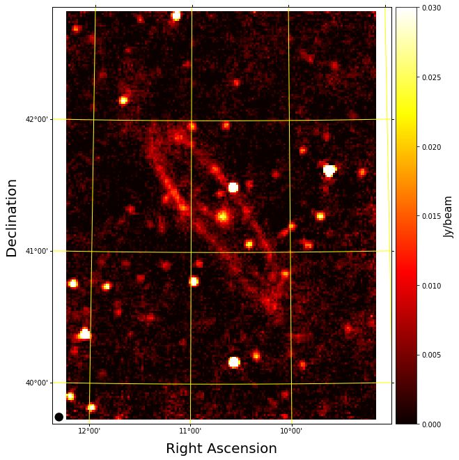
A&A proofs: manuscript no. AA

                      Fig. 1. Left: Final M31 images after averaging over the whole bandwidth at 6.6 GHz. Right: Final M31 image after subtraction of point sources.
                      Both the maps are characterized by an angular resolution of 2.90 . The typical beam size is indicated with the black circle in the bottom-left corner
                      of each panel.

                                                                                                  map, or 1.6 mJy/beam/pixel for the SRT C-band map. Out of the
                                                                                                  all the sources present in the initial NVSS catalog, we detected
                                                                                                  93 counterparts at 6.6 GHz inside the field of the C-band SRT
                                                                                                  map broadly delimited by the black contours in Fig. 2.
                                                                                                       Finally, we merged the CATS catalog with the SRT C-band
                          +42°
                                                                                                  catalog leading to a final list of point sources containing both the
                                                                                                  source positions and all the spectral information available in the
                                                                                                  literature for these objects. The radio spectra of all these compact
DECLINATION (J2000)

                                                                                                  sources were modeled with a modified power:

                                                                                                                         ν
                                                                                                                              !
                                                                                                                                                −log ν ν
                          +41°
                                                                                                  log(F) = −α · log             + log(A) + k · e      re f ,       (2)
                                                                                                                        νre f

                                                                                                  where k is a curvature term, A is the amplitude at the reference
                                                                                                  frequency νre f , and α is the spectral index of the unmodified
                          +40°
                                                                                                  power law. The model converges to the usual power law with
                                                                                                  index α in the limit k → 0. We adopted for reference frequency
                                                                                                  the fixed value νre f = 1 GHz. The observed radio spectra were
                                    12°            11°              10°   9°
                                              RIGHT ASCENSION (J2000)
                                                                                                  fitted with the modified power law model when at least three data
                                                                                                  points were available, otherwise we fixed the curvature to k = 0,
                      Fig. 2. NVSS image at 1.4 GHz with the SRT contours at 6.6 GHz.             resorting to an ordinary power law.
                      Levels start at 2 mJy/beam and increase by a factor of two. The inset             For significantly curved spectra, only the spectral index
                      shows a detail of the M31 ring. The extended emission of the central        between a very close couple of frequencies is meaningful.
                      region (grey area) has been excluded from the point-source search.          Nonetheless, a "local" spectral index value at a given frequency,
                                                                                                  αν , can be easily computed differentiating Eq. 2 with respect to
                      CATS7 (Verkhodanov et al. 1997) database in order to extract the            log νreν f :
                      radio flux density information available in the literature about
                      these sources at other frequencies in the radio band. We then
                                                                                                                       ν
                                                                                                                             !
                                                                                                                                 −log ν ν
                      extracted the flux densities of the point sources present in the            αν = α − k · log               e     re f   .                        (3)
                      6.6 GHz SRT image using as a prior the coordinates of the NVSS                                 νre f
                      catalog. By fitting the same 2D Gaussian + base level model over
                      each one of the NVSS coordinates pairs we obtained the peak                 This can be viewed as the spectral index between an infinitesi-
                      flux density at 6.6 GHz. The fit was performed only if the SRT              mally close couple of frequencies at ν.
                      peak in the NVSS position is > 3σ, where σ is the noise of the                 An example of a spectral fitting of one of the sources is
                                                                                                  shown in Fig. 3. In general, we observe very good agreement
                      7
                           www.sao.ru/cats/                                                       between the SRT flux densities and the measurements from the
                      Article number, page 6 of 36
Fatigoni, Radiconi, Battistelli, Murgia et al.: M31 map at 6.6 GHz

Fig. 3. Fit of the spectrum of the source 4C +39.03 detected in the SRT map. The green open point represents the SRT flux density measurement
at 6.6 GHz. The filled red dots represent the measurements taken from the literature. The values of the "local" spectral indexes at 0.15, 1.4, and 6.6
GHz are also reported. In the right panel we also outline the Planck 857 GHz and the Herschel SPIRE 250 µm 5σ contours in dot-dashed cyan
and yellow, respectively.

literature. Moreover, in Fig. 3 we show that in the case of this
bright source there is also evidence that the SRT in-band spec-
tral index measured at four distinct frequencies between 6.0 and
7.2 GHz is consistent with the trend of both the model fit and the
measurements at nearby frequencies taken from the literature.
     The image of the SRT point-source model at 6.6 GHz is
shown in Fig. 4 at an angular resolution of 2.90 . We recall that
the SRT at C-band point-source model is a subset of the larger
initial catalog based on the NVSS which comprises a larger field
in the sky. Indeed, by using the NVSS-based coordinates and the
best-fit parameters of the modified power law in Eq. 2, it is in
principle possible to generate a point-source model image at any
desired frequency and angular resolution. Moreover, this proce-
dure was followed to remove the point-source contribution from
the global M31 spectral energy distribution (SED) in Battistelli
et al. (2019).
     A catalog of all the compact radio sources in the SRT map
and the best-fit parameters are reported in Table A.1, while in
Fig. A.1 we show all the 93 fits of the spectra. Table A.1 also
reports the spectral indexes measured between 1.4 and 6.6 GHz,
α6.6 GHz
  1.4GHz . The data at 1.4 GHz refer to the NVSS catalog.

4.1. Spectral index distribution                                            Fig. 4. The SRT C-band point-source model.
After obtaining the spectral index      α1.4
                                         6.6 GHz
                                               for each source de-
                                             GHz
tected in C-band, it is possible to study the spectral index dis-
tribution, which is shown in Fig. 5. The average spectral index
value is 0.72, while the median value is 0.81. The spectral index
bin with most occurrences is 0.85 − 0.95.
     As expected, in most cases, the spectral index exhibits a pos-
itive value. Only 2 out of the 93 sources exhibit a negative spec-          synchrotron emission. This population is typically composed of
tral index, or equivalently an inverted spectrum. Approximately             background sources and/or supernova remnants (SNRs) in the
74 % of the sources exhibit a spectral index of α > 0.5, indicat-           M31 field, as has been shown by Galvin & Filipovic (2014) and
ing that their emission is most likely optically thin nonthermal            Lee & Lee (2014).
                                                                                                                        Article number, page 7 of 36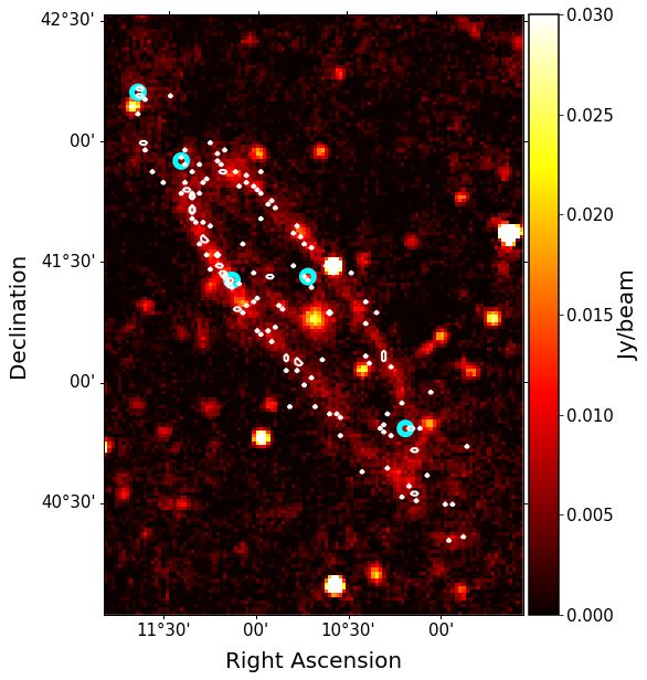
A&A proofs: manuscript no. AA

                                                                           Range (Jy)        Count      Log10 (Diff. Count)       Theor. count
                                                                          0.007 - 0.01        22               6.54                   21
                                                                          0.01 - 0.0135       16               6.33                   14
                                                                          0.0135 - 0.02       15               6.03                   14
                                                                           0.02 - 0.05        14               5.34                   18
                                                                           0.05 - 0.15         5               4.37                    7
                                                                          0.015 - 0.45         3               3.67                    2
                                                                         Table 2. Number of sources detected in C-band map in a given flux
                                                                         density bin. In the last column we show the number of expected sources
                                                                         in each bin from the model we are considering.

Fig. 5. Spectral index distribution between 1.4 and 6.6 GHz for the 93
detected point sources in the field of M31.

4.2. Differential source counts
Given the C-band flux densities for each of the 93 sources, the
differential source counts were computed by binning the 0.007-
0.45 Jy flux density range according to the values reported in
Table 2. It is possible to compare the source counts with a the-
oretical model: here we use the latest version of the 4.8 GHz
model8 by Bonato et al. (2017). As our measurements were per-            Fig. 6. Point-source differential source counts and the fitted power law
formed at 6.6 GHz, we extrapolated them to 4.8 GHz flux density          in double log scale. The error bars parallel to the flux density axis indi-
                                                                         cate the bin widths.
for each source, according to:
                               !α6.6 GHz
                         6.6     1.4 GHz
                                                                              At this point we can compare our source sample with the
F4.8 GHz = F6.6 GHz                        ,                      (4)
                         4.8                                             model from Bonato et al. (2017). This theoretical model returns
                                                                         the predicted Euclidean normalized differential radio source
where α1.4
         6.6 GHz
             GHz is the source spectral index; see Table A.1.            counts per steradian for a discrete series of flux densities. The
    The choice of 0.007 Jy as the lower value to study the differ-       Euclidean normalized differential counts is defined as F 2.5 dNdF ,
ential source counts can be justified assuming a Gaussian dis-           where F is in Jy. In Fig. 7, our source sample is compared with
tribution, an rms value of ∼ 1.6 mJy/pixel within the C-band             the 4.8 GHz model taking into account the ∼ 7 deg2 observed
map extrapolated to 4.8 GHz, and a 3σ peak cut-off. We find              area. The data are in good agreement with the model for the low-
that the sources with flux density of 0.007 Jy are detected with         , intermediate-, and high-density values. The tension in the last
a probability of greater than 95%. It is important to stress that        point in Fig. 7 can be solved by removing from the counts the
a non-negligible fraction (∼ 19%) of the detected sources have           BLAZAR B3 − 0035 + 413 that at 4.8 GHz has an extrapolated
extrapolated flux densities at 4.8 GHz lower than 0.007 Jy; we           flux density of ∼ 0.44Jy.
do not make use of these.                                                     Integrating the model from 0.007 to 0.45 Jy, we find that
    Before comparing the measurements extrapolated to 4.8 GHz            the expected total number of sources is ∼ 76, while in the same
with the source-count model, the source counts n(F) derived              range we detect 75 sources. This appears to confirm the agree-
from
    the  SRT flux densities were fitted with a power law n(F) =        ment between the detected and expected point sources.
    F −γ
A Jy      , where both the number density of sources per flux den-
sity interval at 1 Jy A and the spectral index γ are free parameters.    4.3. The SRT C-band sample of supernova remnants
The result of the fit in logarithmic scale is:
                         !−1.98±0.07                                     With the previously compiled catalog of compact sources de-
dN                    F                                                  tected in our map, we can perform a correlation between SNRs
      = (300 ± 80)                   Jy−1 sr−1 .                  (5)
 dF                   Jy                                                 and SNR candidates in the field of M31. For this purpose, we
                                                                         used the Lee & Lee (2014) SNR and SNR candidate catalog,
    The differential source counts and the best-fit curve are            which includes 156 sources, obtained with Hα and [Sii] images
shown in Fig. 6. The horizontal error bars represent the bin             of M31. Using a 1.450 search radius we cross-matched the SNRs
widths, while the vertical ones correspond to the Poisson error          and SNR candidates catalog with our sample of point sources.
associated with the measurements.                                        The choice of a search radius of 1.450 is motivated by the size of
                                                                         the FWHMS RT = 2.90 . We found then that source numbers 241,
                                                                         359, 622, 626, and 645 have at least one corresponding source
                                                                         in the SNR catalog. In particular, for the SRT source number
8
    http://w1.ira.inaf.it/rstools/srccnt/                                645 we have four corresponding sources within 1.450 , three cor-
Article number, page 8 of 36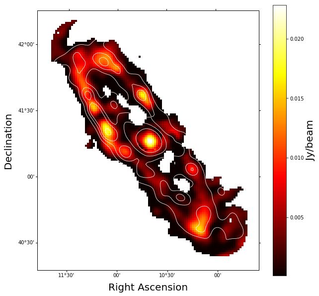
Fatigoni, Radiconi, Battistelli, Murgia et al.: M31 map at 6.6 GHz

                                                                              SRT source n.      Lee SNR n.     Distance(0 )   α6.6 GHz
                                                                                                                                1.4 GHz
                                                                                  241                50            0.87         0.42
                                                                                  359                17            0.93         0.49
                                                                                  622               156            0.96         0.16
                                                                                  626               144            0.78         0.31
                                                                                  645                97            0.09         0.01
                                                                        Table 3. The SRT C-band sources with a correspondence in the Lee et
                                                                        al. (2014) catalogue.

Fig. 7. Normalized differential point-source counts compared with the
Bonato et al. (2017) model at 4.8 GHz.

responding sources for the SRT source number 622, and 2 for
number 241. The other two SRT sources have only one corre-
sponding source each. In Fig. 8 we show all the 156 SNRs and
SNR candidates (white contours) and the sources that have a cor-
responding source within a radius of 1.450 (cyan circles).

                                                                        Fig. 9. The SRT C-band map of M31 with selected Hii region contours.
                                                                        We note the remarkable agreement between the distribution of the Hii
                                                                        regions and the location of the 10 kpc ring and the 15 kpc structure.

                                                                        the same 1 GHz amplitude, it is much more likely to detect the
                                                                        source with a flat spectrum than the source with a steeper one.

                                                                        5. M31 morphology
                                                                        Studies of M31 have revealed a normal disk galaxy with spi-
                                                                        ral arms wound up clockwise. The spiral arms are separated
                                                                        from each other by at least 4 kpc. The spiral pattern is some-
                                                                        what distorted by the interactions of the galaxy with M32 and
                                                                        M110 (Gordon et al. 2006). The Spitzer Space Telescope (SST)
                                                                        revealed two spiral arms emerging from a central bar. The arms
Fig. 8. The SRT C-band map with compact sources. The 156 SNRs           have a segmented structure and continue beyond the galaxy’s
and SNR candidates from (Lee & Lee 2014) are overplotted with white     ring mentioned above. The ring shape of M31 was discovered
contours. The SRT sources that have a corresponding source within a     in the 1970s (Pooley 1969; Berkhuijsen & Wielebinski 1974).
radius of 1.45’ are shown with cyan circles.                            Comparing the radio emission at 6.6 GHz and the location of
                                                                        the 3691 Hii regions presented in Azimlu et al. (2011) we find
     In Table 3 we report the list of sources with a match in the       a strong correlation in the ring, as one can see in Fig. 9. The
Lee & Lee (2014) catalog, together with the ID in that same cata-       Hii level contours denote 1, 3, or 6 Hii regions inside each SRT
log, the distance from the center, and the spectral index between       C-band pixel, and so they are not flux density contours but are
1.4 and 6.6 GHz.                                                        simply an indication of the positions of the Hii regions.
     We note that the sources with a corresponding source in the            The ring structure is believed to be the result of the inter-
SNR catalog are mostly characterized by a relatively flat spec-         action with M32 over 200 million years ago. The M32 galaxy
trum. This is a bias most likely introduced by the achieved sen-        likely passed through the disk of M31, which left M32 stripped
sitivity at 6.6 GHz with SRT: if we assume two sources with             of more than half of its mass (D’Souza & Bell 2018). The nu-
                                                                                                                 Article number, page 9 of 36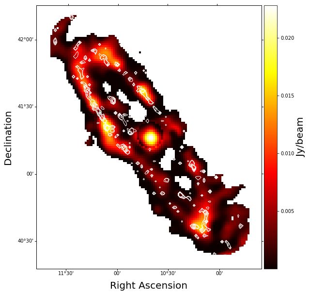
A&A proofs: manuscript no. AA

cleus of M31 is home to a dense, compact star cluster. A total         ring and in the central region, we can also find small patches (vi-
of 35 black holes have been detected in M31, of which 7 are            olet and blue pixels) not located at the edge of the map where the
within 0.3 kpc of its center (Barnard et al. 2013). These black        SRT and Effelsberg S/N is lower, with a spectral index around
holes formed by gravitational collapse of massive stars and have       α = 0.4 − 0.5. These are the regions where thermal free-free
a mass of between approximately five and ten times that of the         emission is expected to be dominant and are likely to be Hii
Sun.                                                                   regions, which are mainly located in these parts of the galaxy,
     Radio and microwave observations revealed emission from           as shown in Azimlu et al. (2011). In some inner and outer
the central region and only from the external ring, while the cen-     ring regions we find that the spectral index is larger than 0.9.
tral bar is not detected. The central bar, which is detected in all    This means that these regions are characterized mostly by syn-
the IR images, is also not visible in the ancillary Effelsberg radio   chrotron emission, with the steep slope indicating that an old
maps. As one can clearly see in Fig. 9, the 10 kpc ring and the 15     population of electrons is responsible for the nonthermal emis-
kpc structure, noted in IR maps, (Haas et al. 1998; Gordon et al.      sion.
2006) are well correlated with the location of the Hii regions in          Spectral index maps of M31 have been built before (Berkhui-
the SRT map. The 15 kpc structure is unfortunately at the edge         jsen et al. 2003; Beck et al. 2020). We find excellent agreement
of the Effelsberg maps, and in the following section, when these       between our spectral index map shown in Fig. 10 and the one
maps are used, it is not possible to disentangle thermal and non-      extracted by Berkhuijsen et al. (2003) , which is not surprising
thermal emission within these external regions.                        given the fact that, with the exception of the SRT C-band map,
     The M32 and NGC205 galaxies, which fall inside the SRT            to extract the spectral index we used the same set of maps, at
coverage, are not detected because of their low radio emission.        the same angular resolution. The spectral index values found by
Brown et al. (2011) found that, at 1.4 GHz, M32 and NGC205             Beck et al. (2020) using Effelsberg maps at 1.465 and 8.350 GHz
have respectively a flux density of 0.7 ± 0.5 mJy and 0.1 ± 0.5        are generally smaller than ours by 0.2-0.3. We can ascribe this
mJy. Also, if a flat radio spectral index is assumed for these         discrepancy to the difference in total flux density between the
galaxies (most favorable scenario), their flux densities are           SRT 6.6 GHz map and the new Effelsberg 8.35 GHz map. More
compatible with the SRT confusion noise and therefore cannot           specifically, the latter shows a flux density that is ∼ 15% higher
be detected.                                                           than the former. We identified some factors that could account
                                                                       for this discrepancy:
    In the following, we investigate the M31 radio features by
                                                                        – The point sources in the two maps have been subtracted with
creating a spectral index map, and by studying the spectral index
                                                                          different methods. Residual point sources in one map that
trend within the central region and the entire galaxy.
                                                                          have been removed from the other can affect the flux differ-
                                                                          ence in both directions.
5.1. Spectral index map                                                 – Maps have been made with different telescopes, the data have
                                                                          been analyzed independently, and different software has been
We start by building a spectral index map across the whole M31.           used.
In general, a flat spectral index is expected in regions whose          – The total area covered by the two maps is different; this can
emission is dominated by a thermal component, while a steeper             affect the background estimate and the baseline subtraction.
spectrum is an indication of a substantial presence of nonthermal
emission.                                                                   Moreover, Battistelli et al. (2019) showed that AME is the
    The spectral index value has been calculated on a pixel-           dominant emission mechanism in M31 in the frequency range
by-pixel basis by taking into account only the pixels with flux        10-60 GHz. This means that, at 8.35 GHz, AME must make up
densities greater than 3σ in all considered maps, where σ is           10 − 15% of the total integrated flux density, causing the spectral
the map sensitivity expressed in Jy beam−1 . Indeed, pixels            trend to drift away from a simple power law. Therefore, AME
below this threshold are those where the spectral index becomes        can account for part of the difference between the two spectral
very uncertain because of the presence of faint radio emission         index maps.
and radio noise. The spectral index map was created using                   In the following sections, we explain how we used our spec-
Effelsberg maps at 1.46 GHz and 4.85 GHz and the SRT map at            tral index map to choose regions in which to perform a detailed
6.6 GHz. We used the maps projected and then convolved to 30           study of the decomposition between thermal and nonthermal
as explained in Sect. 3.                                               emissions.

    The spectral index value and its 1σ uncertainty were com-          5.2. Spectral index trend
puted pixel by pixel by fitting the relation:
           ν −α                                                      Hereafter, we evaluate the spectral index gradient across the
                                                                       galaxy and, in doing so, we separately analyze the properties of
f (ν) = A            ,                                     (6)
           1 GHz                                                       the central region. For this analysis we used the Effelsberg map
                                                                       at 2.7 GHz and all the other radio maps projected and convolved
where both A and α are free parameters. To perform the                 to 50 as explained in Sect. 3. We fitted a simple power law with
fitting, we used a Python implementation of Goodman and                two free parameters using the integrated flux densities in each
Wear’s Markov chain Monte Carlo (MCMC) Ensemble sampler                given region instead of single pixel values, following the same
(Foreman-Mackey et al. 2013). The same MCMC was used in                procedure for the extraction of the spectral index map.
the following sections, to fit the emission in the central region          For the galaxy central region, we evaluated the spectral
and that in the ring, and to disentangle thermal and nonthermal        index within four concentric rings centered at (Ra, Dec) =
emission maps. The spectral index map and its 1σ uncertainty           (10.70, 41.28) deg (see Table 4 for more details). For each ring,
are shown in Fig. 10.                                                  the total flux density was evaluated as:
     Globally, the spectral index map shows values of α ' 0.7
(light blue and light green pixels). In the northern and southern      F = S̄ in − S̄ ext Ωin ,                                      (7)
Article number, page 10 of 36
Fatigoni, Radiconi, Battistelli, Murgia et al.: M31 map at 6.6 GHz
Fig. 10. Left panel: Spectral index map extracted from 1.46 and 4.85 GHz Effelsberg maps and our SRT 6.6 GHz map. Right panel: Spectral index
1σ noise map. The typical beam size (FWHM= 2.90 ) is indicated with the black circle in the bottom-left corner of each panel.
Ring n. Galactoc. Spectral σ Ring n. Galactoc. Spectral σ
Distance(kpc) Index S.Index Distance(kpc) Index S.Index
1 0-0.34 0.62 0.14 1 0-1.13 0.66 0.05
2 0.34-1.02 0.63 0.10 2 1.13-3.40 0.90 0.05
3 1.02-1.70 0.68 0.09 3 3.40-5.66 1.05 0.04
4 1.70-2.38 0.77 0.09 4 5.66-7.92 0.94 0.04
Table 4. Spectral index values in the central region as a function of 5 7.92-10.18 0.83 0.04
galactocentric distance. 6 10.18-12.45 0.87 0.05
7 12.45-14.14 1.01 0.05
Table 5. Spectral index values as a function of the galactocentric dis-
tance for the whole galaxy.
where S̄ in is the brightness inside the integration region, S̄ ext is
the background brightness and Ωin is the solid angle subtended
by the region. The thermal brightness uncertainty was computed
as explained in Rubiño-Martín et al. (2012) and then combined presents smaller values with respect to the peak reached within
with the calibration error9 . the third ring. The average value of ∼ 0.9 found at distances
The spectral index as a function of distance from the galaxy greater than ∼ 4 kpc strongly hints at synchrotron emission be-
center and the four rings where it was calculated are shown in ing the predominant mechanism at these frequencies. The point
Fig. 11. For each ring we used a position angle of −52 deg in the at highest galactocentric distance corresponds to the edge of the
(Ra, Dec) system and an eccentricity equal to 0.26. The spectral ring: as expected, because of the aging of electrons, we found a
index within the central region is found to be approximately con- steeper spectral index value. The same spectral index trend and
stant within the uncertainties. We further investigate the central similar values have been found by Berkhuijsen et al. (2003).
region emission in Sect. 6.1 by decomposing thermal and non-
thermal emission.
We also repeated the same analysis for the whole galaxy: in
this case we used seven elliptical rings, centered at (Ra, Dec) = 6. Thermal versus nonthermal emission
(10.70, 41.28) deg, with the same position angle and eccentric-
ity as those used for the central region. The details of the seven In this section we report a full decomposition of the M31 emis-
regions and the spectral index values are reported in Table 5. sion into thermal and nonthermal components. We start by an-
The seven elliptical rings and the spectral index as a func- alyzing the central region and the full 10 kpc ring individually,
tion of the distance from the galaxy center are shown in Fig. 12. and then the northern and the southern halves of the 10 kpc ring
The spectral index shows a clear positive gradient in the inner- individually as well (Fig. 13). It is interesting to conduct a sep-
most 6 kpc (first three rings). In the outermost rings, the gradient arate analysis on the latter two regions because they appear to
changes sign twice, at ∼ 6 (decreasing) and at ∼ 10 kpc (in- have different properties in the spectral index map.
creasing again), even though the values are compatible with a For this decomposition, we used the maps reported in Table
flat trend between ∼ 8 kpc and ∼ 12 kpc. Overall the 10 kpc ring 6, all projected to the SRT C-band map coordinate system and
convolved to a resolution of 50 . For all the regions mentioned
9
The calibration errors are considered to be 5% for all the maps. above, the flux densities were fitted with a synchrotron+free-free
Article number, page 11 of 36A&A proofs: manuscript no. AA
Fig. 11. Upper panel: Four elliptical rings used to compute the spectral Fig. 12. Upper panel: Seven elliptical rings used to compute the spec-
index trend with the distance from the center of M31. Lower panel: tral index trend with the distance from the galaxy center. Lower panel:
Spectral index average radial profile calculated within the rings shown Spectral index average radial profile calculated within the rings shown
above. above.
model with three free parameters: the free-free and synchrotron A summary of the flux densities we used as data points for
amplitudes at 1 GHz, and the synchrotron spectral index. the fit, divided by region, is reported in Table 6, where the re-
ported flux density uncertainties are a combination of statistical
and calibration errors. A summary of the fit results is reported in
F sync (ν) = A sync ν−αsync , (8) Table 7.
Finally, in Sect. 6.5 we carry out a detailed separation into
components, pixel by pixel, for the whole galaxy and produce
F f − f (ν) = A f − f T e−0.5 g f f . (9) thermal and nonthermal emission maps.
We used Eqs. 8 and 9 to describe synchrotron and free-free
emissions, respectively. The electron temperature T e in Eq. 9 has 6.1. Central region
been fixed at 8000 K throughout the paper. Fixing the electron
temperature is not fundamental in the decomposition between In order to evaluate the total flux density in the central area, we
thermal and nonthermal emission because the free-free ampli- used a circular region centered at (Ra, Dec) = (10.70, 41.28) deg
tude is left as a fit parameter, but it is important in the SFR ex- with a radius of 60 .
traction. In the latter case, we fix T e = 8000 K as we expect the In Fig. 14 we show the data points and the thermal, nonther-
10 kpc ring to host most of the M31 star forming regions (Ford mal, and total emission fit models. The final χ2 is 4.0. According
et al. 2013) and we know that in our Galaxy the electron temper- to the fit, at 1 GHz, the thermal emission within the central re-
ature at around a galactocentric distance of 10 kpc is ∼ 8000 K gion is about ∼ 8% of the total emission, while extrapolating the
(Paladini et al. 2004). flux density to the SRT C-band frequency we conclude that the
Article number, page 12 of 36You can also read