REPORT REPORT Summer Peak Shaving Adjustment Resources in PJM - Prepared for CAPS - Nccdn.net
←
→
Page content transcription
If your browser does not render page correctly, please read the page content below

REPORT

       Summer Peak Shaving Adjustment Resources
                                       REPORT in PJM

Prepared for CAPS
By Demand Side Analytics, LLC
March 2019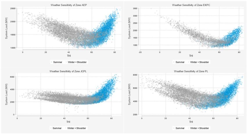
PREPARED BY
Jesse Smith, Principal Consultant
Adriana Ciccone, Senior Consultant
Ross Beppler, Quantitative Analyst
TABLE OF CONTENTS
1 PJM Summer Only Demand Response Task Force Outcomes ......................................................... 3
1.1 LOAD FORECAST ADJUSTMENT ........................................................................................................... 3
1.2 DESIGN COMPONENTS AS ADOPTED .................................................................................................... 4
1.3 TIMELINE ......................................................................................................................................... 6
2 Peak Shaving Resource Offer Strategy ........................................................................................... 7
2.1 WEATHER ........................................................................................................................................ 8
2.2 SYSTEM LOAD CHARACTERISTICS .......................................................................................................10
2.3 CUSTOMER ROTATION ...................................................................................................................... 13
3 Valuation of Peak Shaving Adjustments ....................................................................................... 14
3.1 THE ECONOMIC THEORY OF CAPACITY PRICE SUPPRESSION...................................................................14
3.2 MODELING OF PJM BRA SENSITIVITY ANALYSES ................................................................................. 15
3.3 AVOIDED COST OF TRANSMISSION AND DISTRIBUTION CAPACITY .......................................................... 19
4 Conclusions and Recommendations ............................................................................................. 20
Figures
Figure 1: VRR Curve with Peak Shaving Adjustment ............................................................................... 4
Figure 2: Sample Program Decision Chart ............................................................................................... 8
Figure 3: Distribution of Average Number of Summer Events by THI Trigger .......................................... 9
Figure 4: Distribution of Events by Month and Zone ............................................................................. 10
Figure 5: Peak Forecast Impact as a Share of Shaving Amount by Zone .................................................11
Figure 6: Weather Sensitivity of Select PJM Zones ............................................................................... 12
Figure 7: System Load Characterization .................................................................................................13
Figure 8: Price Suppression Example..................................................................................................... 15
Figure 9: RTO Capacity Supply Curve Slope Estimation from BRA Scenario Analysis 2021/2022 .......... 16
1|P a g e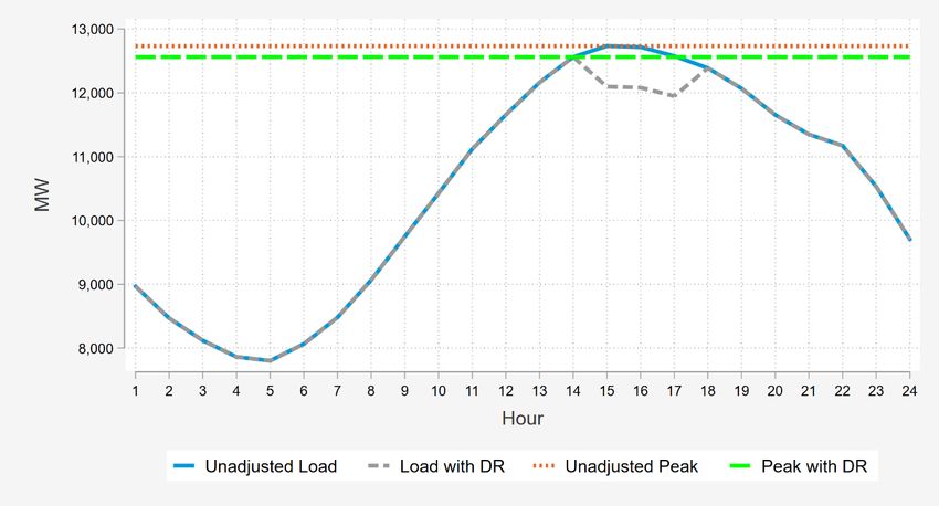
Figure 10: Supply Curve Slope Approximations from RTO Base Residual Auction Scenarios by Year ..... 17
Figure 11: Supply Curve Slope Approximations from EMAAC Base Residual Auction Scenarios by Year 17
Figure 12: Distribution of Events for Cool, Average, and Hot Summers – 81 THI Threshold................... 22
Figure 13: 600 MW Shaving Program with Three Hour Events – ATSI Zone........................................... 23

Tables
Table 1: Peak Shaving Adjustment Program Design Components .......................................................... 5
Table 2: Hypothetical PSA Value Calculation ........................................................................................ 18
Table 3: THI Thresholds for a Mean of 24 Shaving Hours per Summer .................................................. 21

                                                                                                                         2|P a g e
1 PJM SUMMER ONLY DEMAND RESPONSE TASK
  FORCE OUTCOMES
At its October 25, 2018 meeting, the Markets and Reliability Committee of PJM voted in favor of a
motion to adopt PJM’s proposal for creation of a Peak Shaving Adjustment mechanism. The proposal
was the result of work by the Summer Only Demand Response Task Force (SODRSTF) which sought to
explore mechanisms to include summer only DR resources in PJM’s forward capacity market (Reliability
Pricing Model, or RPM). Historically demand resources such as demand response and energy efficiency
have entered the market as supply and been eligible to compete alongside traditional supply side
resources (power plants) in a competitive auction to fulfill the resource requirements for the region.

Demand response resources such as utility direct load control of central air conditioners have recently
encountered difficulty participating in the market due to PJM’s “capacity performance” definition of
generation capacity. Capacity Performance, or CP resources, must be able to perform 16 hours per day
for consecutive days on any operating day regardless of season, weekends, or holidays. While summer
only resources could theoretically pair with a winter only resource to form a bid, EDCs and LSEs with
existing summer only DR resources perceived the move to Capacity Performance would lead to
stranded summer assets in a summer-peaking system. The SODRSTF charter directed the task force to
explore mechanisms to value demand response for those resources that may not be able to clear in the
capacity market.

Over the course of nine months, SODRSTF members brought forth various proposal packages with
different design components. Through a collaborative process, PJM adjusted its proposal to include key
elements of other packages and ultimately received 65% support from the task force.

1.1 LOAD FORECAST ADJUSTMENT
A Peak Shaving Adjustment (PSA) is fundamentally different from the way demand response has
participated in RPM historically. Instead of being treated as supply that is capable of fulfilling resource
requirements, a Peak Shaving Adjustment enters the market on the demand side. In PJM’s capacity
market, demand is represented by the Variable Resource Requirement (VRR) curve. As shown in Figure
1, the VRR curve is downward sloping. The resource clearing price is ultimately the coordinates on the
y-axis (price), where the supply curve – which is upward sloping – intersects the demand curve. Figure 1
also shows the underlying mechanism by which Peak Shaving Adjustments will be recognized in the
market. Once recognized by PJM, Peak Shaving Adjustments will lower the peak load forecast for a
zone and move the VRR curve to the left.

                                                                                                 3|P a g e
Figure 1: VRR Curve with Peak Shaving Adjustment
The amount a Peak Shaving resource will lower the summer peak load forecast and move the VRR
curve the left is a function of several factors.
The amount of load reduced when active (MW)
The frequency of shaving (number of days per summer)
The duration of shaving (number of hours per day)
Zonal load characteristics also affect the magnitude of the load forecast adjustment and are discussed
in more detail in Section 2.1. The load forecast adjustment itself is calculated by PJM using the
difference in two forecast models.
1. Traditional econometric load forecast using historic loads, weather, and other factors
2. The same model with a modified load history. Using the attributes provided by the program
administrator, PJM will subtract the expected shaving from historic loads back to 1998 and
re-run.
1.2 DESIGN COMPONENTS AS ADOPTED
Table 1 summarizes the key design components of the Peak Shaving Adjustment mechanism. The table
is adapted from a proposal matrix compiled by PJM to compare packages in the SODRSTF.
4|P a g e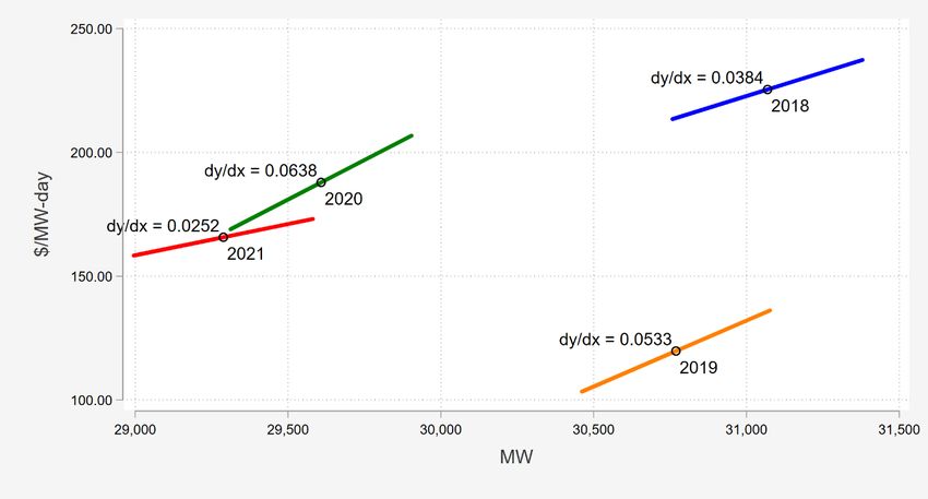
Table 1: Peak Shaving Adjustment Program Design Components

          Design Component                                                               Description
                                     Forecast Adjustment based on load forecast run for BRA with modified load history that assumes anticipated
Mechanism to recognize summer
                                     curtailment behavior occurred in the past. VRR curve is reflective of the reliability requirement, which depends on
only DR
                                     the load forecast and the monthly load profile.
                                     Economic DR rules, which use a customer baseline (CBL). CBLs use average load data from recent non-event days
Measurement and Verification (M&V)   to estimate what load would have been absent curtailment. The default CBL is a “high 4 of 5” with SAA. PJM
                                     Manual 11 provides a full list of potential CBLs.
                                     Modification to forecast adjustment based on most recent performance. If a resource under-performs relative to
Non-Performance Penalties
                                     its commitment, subsequent commitments will be de-rated.
                                     Temperature Humidity Index (THI) as determined by the program administrator. This is different from traditional
                                     DR in that there is no event “call”. The program administrator must monitor weather conditions and determine
Curtailment Trigger
                                     whether to shave or not based on the weather forecast. The THI trigger is a daily maximum – actual, not
                                     forecasted. Section 2.1 includes addition discussion of weather considerations.
                                     Function of the lower forecast and shifting the VRR curve left. No compensation is provided. The zone only lowers
Capacity Market Valuation            the amount of capacity they are obligated to purchase (an avoided payment). All benefits accrue to the zone in the
                                     form of a reduced capacity obligation.
                                     Program Administrator (EDC, LSE, CSP, State or Other) is fully responsible to fulfill the load forecast adjustment
Supervisory Control                  requirements. Program Administrator manages a portfolio of customers under an approved Relevant Electric
                                     Retail Regulatory Authority (RERRA) tariff or Order.
                                     Pre-determined. Program administrators can select any active months they wish and communicate that to PJM.
Performance Months
                                     Affects the valuation.
Interruption Days                    Unlimited. Any non-holiday weekday in the performance months
                                     Pre-determined. Program administrator decides which hours they will shave load on days the THI trigger is met
Interruption Hours
                                     and communicates that to PJM. Affects valuation.
                                     Load reduction programs governed by tariffs/orders. Dual participation in supply-side DR (Economic or Load
Eligibility
                                     Management) or PRD is not allowed.
Timeline for reporting program
                                     10 business days prior to September 30th. Timeline is adjusted for transition period (see Section 1.3)
components to PJM
Applicable Auctions                  Base Residual Auction and Incremental Auctions

                                                                                                                                                  Page | 5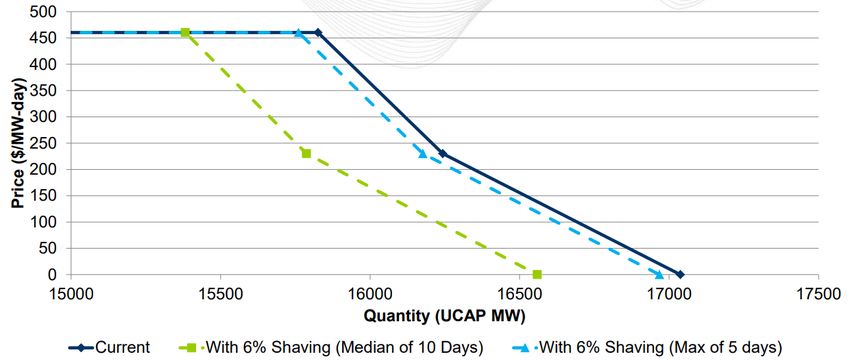
The design components listed in Table 1 were not unanimous and alternate structures will likely be
proposed until all rulemaking is final at PJM and FERC. The two areas that received the most attention
during the SODRSTF meetings were:
1) Eligibility – several package sponsors sought alternatives to the PJM package design that
disallows participation as both supply and demand in the market.
2) Supervisory Control – some package sponsors felt that specifying Program Administrators
must manage customers under RERRA tariff or Order was too restrictive and would limit access
to Peak Shaving Adjustment market opportunities.
All of the components in Table 1 are important for states and program administrators to understand
and consider when nominating a Peak Shaving Adjustment. The prohibition of dual participation may
prove especially important for some states. While residential customers do not participate in supply-
side DR absent aggregation by EDCs or program administrators, large C&I customers do. For example,
Pennsylvania’s Act 129 demand response programs deliver 450-500 MW of peak shaving on hot
summer afternoons. However, many of the large industrial customers that participate in this state
program also have commitments in PJM DR programs (as supply). Regulators and EDCs in Pennsylvania
would have to carefully consider the amount of eligible peak shaving capability in existing programs
before nominating a Peak Shaving Adjustment.
One issue we expect will require additional clarification moving forward is the eligibility of peak
demand reductions associated time-varying pricing (TVR). Peak time rebates (PTR) are a dispatchable
type of rate and were discussed in the SODRSTF as eligible. We believe event-based price signals such
as critical peak pricing (CPP) would also be eligible. The case for new ‘everyday’ time-of-use rates or
residential demand charges is less clear. Certainly these strategies provide a price signal to shave peak
demand, but they are not dispatchable. A downward adjustment in the peak demand forecast seems
like a logical place to reflect the expected effects of TVR, but PJM will need to determine how long such
deployments are considered a load forecast adjustment and at what point they become embedded in
the default load forecast.
1.3 TIMELINE
The commitment cycle for Peak Shaving Adjustments (PSAs) will precede the Base Residual Auction for
generation capacity. The BRA for a delivery year is held in the spring, three years prior to the delivery
year. For example, the BRA for the 2021/2022 delivery year (June 1, 2021 to May 31, 2022) was held in
May 2018. The BRA for the 2022/2023 delivery is delayed until August 2019 because of FERC filings so
the Peak Shaving Adjustment timeline is different as it is phased into place. Once the transition period
is complete, PSAs will need to commit by the September prior to the BRA – or almost four years before
the delivery year. Key dates for the 2022/2023 delivery year are:
December 2018 – PJM releases it’s 2019 Peak Load Forecast. This forecast will not reflect
any adjustments for Peak Shaving
February 1, 2019 – PSA program parameters must be submitted to PJM
Page | 6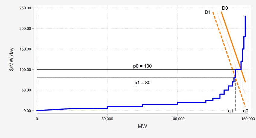
March 15, 2019 – PJM publishes a new Peak Load Forecast inclusive of Peak Shaving
Adjustments
May 1, 2019 – Planning parameters for the 2022/2023 BRA are posted online
August 2019 – Base Residual Auction of the 2022/2023 delivery year occurs
June 1, 2022 – Beginning of the 2022/2023 delivery year. PSAs nominated in February 2019
are expected to perform when the THI trigger is met.
The timeline listed above may ultimately be delayed as FERC approval of the PJM proposal has not
been finalized. In February 2019, FERC issued a letter of deficiency to PJM citing the need for additional
clarity on several topics. This development has timeline implications because it reopens the filing for
member comments and also allows for time periods for PJM to address the topics and for FERC to
review.
Specifics aside, a key aspect of this timeline is that PSAs commit in advance of the auction which sets
the resource clearing price (RCP). This means a PSA must commit to peak shaving activity without
knowing what the value of that shaving will be. Program administrators will have to look at historic
clearing prices and base decisions to commit on estimate values. There is no mechanism to withdraw a
commitment based on price, other than non-performance.
Another key takeaway from the timeline shown above is that PSAs must commit well in advance of
delivery. This can create challenges for utility or state planning cycles which sometimes set program
plans, budgets and goals in 3-5 year cycles, but only plan 1-2 years in advance. As shown in Table 1,
PSAs can also commit in Incremental Auctions, but clearing prices in Incremental Auctions have been
lower than BRAs historically.
2 PEAK SHAVING RESOURCE OFFER STRATEGY
The valuation of a Peak Shaving Adjustments will be dependent on the magnitude, frequency, and
duration of peak shaving. A program administrator that commits to shave 100 MW for two hours per
day on summer weekdays with a maximum THI of 84 might receive a 20 MW reduction in their summer
peak load forecast and reliability requirement. If the same program administrator were to commit to
shave 100 MW for six hours per day each weekday the maximum THI exceeded 78, the zone might
receive an 80 MW load forecast adjustment.
Figure 2 illustrates the fundamental decision a program administrator must make when nominating a
PSA resource. Along the x-axis is THI. The blue bars show the expected number of peak shaving days
per summer at each THI trigger and are based on 20-year averages for a hypothetical zone. Of course
not every year exhibits average weather. The orange, green, and yellow lines represent the valuation of
a PSA for given event duration. The valuation percentages can be thought of as the percentage of a
resource clearing price the PSA earns. Consider a 100 MW PSA that is allocated a 60 MW reduction in
resource requirement (60%) for a delivery year where the resource clearing price is $100/MW-day. That
100 MW peak shaving program is valued at 60% of the clearing price, or $60/MW-day.
7|P a g e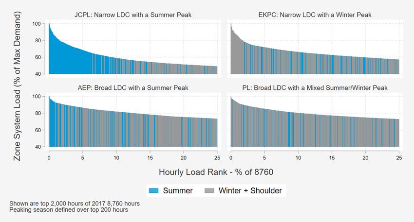
Figure 2: Sample Program Decision Chart
60 100%
Mean Events per Summer
Load Forecast Adjustment (% of Shaving MW)
55 90%
Valuation - 6 hour events
50
Valuation - 4 hour events 80%
Expected Events per Summer
45
Valuation - 2 hour events
70%
40
35 60%
30 50%
25 40%
20
30%
15
20%
10
5 10%
0 0%
75 76 77 78 79 80 81 82 83 84 85
THI Threshold
The height of the blue bars is a function of weather conditions which have to be estimated based on
historic data. Section 2.1 explores the risks and decision criteria associated with weather. The shape of
the orange, green, and yellow lines illustrated in Figure 2 for a given zone is also a function of zonal load
characteristics. This is explored in more detail in Section 2.2.
2.1 WEATHER
Peak Shaving days will be identified based on the maximum Temperature-Humidity Index (THI) that a
system reaches on any given summer weekday. Program administrators must select a THI threshold for
their Peak Shaving program and must dispatch the program whenever that THI threshold is met. This
design has uncertainty associated with it, and administrators should understand how weather
variability affects program operations. There are two main types of uncertainty related to weather that
should be considered:
Weather forecasts are not error-free. For example, during summer months in the Mid-
Atlantic region, afternoon thunderstorms can lead to lower observed THI values compared
to forecasts.
Observed weather varies from year to year. Whether a summer will be a hot or mild
summer cannot be known in advance.
Without a detailed study of weather forecast accuracy, it is difficult to say what the impact of forecast
error would be on program dispatch. Program administrators should consider if setting an internal THI
trigger lower than the committed trigger to avoid missing a shaving day if the observed THI is higher
8|P a g ethan forecasted. Since a lower THI threshold would mean more events, which can have customer
incentive and participation implications, program administrators should weigh these costs against any
penalties for underperformance. Program administrators will also need to consider when to make
“go/no-go” decisions regarding peak shaving. Waiting as close as possible to the committed shaving
hours will reduce uncertainty, but also limits the opportunity for “pre-cooling” of homes for programs
that shave via control of central air conditioning loads.
Year-to-year variations in weather are easy to understand using historic data. Figure 3 shows the
distribution of events per summer for the JCPL (Jersey City Power & Light) system across a range of THI
triggers. This graph is a box-and-whiskers plot that illustrates the distribution of a given metric – in this
case the number of event days per summer (based on weather data from 2006 to 2017). The height of
the blue rectangle (box) illustrates the range of the 25th through 75th percentile of event days per
summer, so for example we can see that 50% of summers would have between about 10 and 15 events
per summer if the THI trigger had been set to 81. The median outcome in that example is where the line
in the middle of the blue rectangle is, or about 12 shaving days per summer. The more salient values
from the chart, however, are the minimum and maximum observations that are shown either as the
minimum and maximum range of the whiskers, or as the points outside the whiskers, which are
classified as outliers. So while, with a THI of 79, the JCPL system experiences a median of 22 events per
summer, the lowest number of peak shaving days per summer that would have been observed in this
twelve-year period was 8 peak shaving events. Perhaps most importantly for program planners, the
highest year would have had 35 shaving events.
Figure 3: Distribution of Average Number of Summer Events by THI Trigger
9|P a g eWhat this means for program administrators is that, while a program may be designed at a particular
THI trigger to yield an average or median number of events in a summer, the intrinsic variability in year-
to-year weather variability will result in unpredictable numbers of events.
Complicating these decision points further, this variability is not necessarily evenly distributed
throughout the summer. Figure 4 shows the average number of events per month across all PJM zones
and summer months. Naturally, the hotter and more humid months of July and August trigger more
shaving events at any THI threshold, and the higher the threshold, the fewer events there are overall.
However, such intra-seasonal variability may have effects on participation. It is one thing to enroll in a
program that is expected to deliver 20 events per summer, however it may be another to have half of
them triggered in a single month.
Figure 4: Distribution of Events by Month and Zone
2.2 SYSTEM LOAD CHARACTERISTICS
Not every system will have the same peak load forecast impact given the same program design. Due to
unique characteristics for each zone, a program that shaves for 5 days a summer in JCP&L will have a
higher impact on the peak load forecast than nearly any other system in PJM, as shown in Figure 5.
Similarly, the difference in forecast impact between a program that shaves for a maximum of 5 days per
summer compared to one that shaves a median of 10 days per summer can vary by system. These
10 | P a g edifferences are motivated by system load characteristics that make each territory unique. In this
section, we examine the key drivers of peak load forecast impact, and what design features of a peak
shaving program affect impacts.
Figure 5: Peak Forecast Impact as a Share of Shaving Amount by Zone
Every system in PJM has slightly different characteristics, due to its size, weather, diversity of industry
and residential composition. These differences have meaningful implications for the ability of a
summer peak shaving program to lower the reliability requirement for the zone. To assess the value of
such a peak shaving program, we should first consider two important interactions between the system
and the program:
1) Does the system typically peak when summer peak shaving events would be called?
2) Will the peak shaving activity create a new peak or broaden the peak substantially and spread
risk across other days and hours when shaving does not occur?
The first question can be considered in two ways. First, does the system even peak in the summer,
when the peak shaving program is operational? Is the zone a summer-peaking, winter-peaking, or dual
peaking system? Second, for a given THI trigger, is the system at its peak demand? That is, if an event is
called, what is the likelihood that the system is at its peak? Figure 6 shows how these characteristics
can change by zone. On the y-axis is an hourly system load for one of four systems for calendar year
2017. The x-axis shows the THI in that interval. Finally, the markers are color coded for summer/non-
summer months. For some systems, the maximum system load occurred in the summer, such as AEP
(American Electric Power) and JCPL (Jersey City Power & Light). EKPC (East Kentucky Power
Cooperation) clearly peaks strictly in the winter, while PL (PPL) is relatively balanced in peaking
between summer and winter and the season the peak occurs may vary from year to year based on
weather.
11 | P a g eFigure 6: Weather Sensitivity of Select PJM Zones
Systems that peak in the summer will be allocated more value from a summer-only DR program, as
demand reductions will reduce the overall system peaking risk and generation capacity requirement for
the zone. Figure 6 also shows differing levels of variability in system load at a given THI. AEP and JCPL
are both summer-peaking systems, however at a given THI, AEP has a much broader range of observed
system load than JCPL. Similarly, we see AEP loads at or near the maximum system load for the year at
several degrees lower than the observed maximum THI. Based on these characteristics, we’d expect the
same amount of peak shaving based on a THI threshold to yield a smaller reduction in the peak load
forecast than for JCP&L.
To assess the second question, it is also helpful to look at a system’s load duration curve (LDC). The LDC
ranks system load in descending order, and in some cases normalizes it to be compared to other
systems. Shown below in Figure 7 are normalized load duration curves for four illustrative PJM systems.
The y-axis is defined as the % of the maximum demand in that year and the x-axis is the rank of each
hour-long interval as a percent of the 8,760 hours in a year. Each interval is color-coded in either blue or
grey to indicate which season that interval comes from – either Summer (May – September) or Winter
& Shoulder (all others). As discussed above, both Jersey City Power & Light and American Electric
Power peak in the summer months, while East Kentucky Power Cooperative peaks in the winter and
PPL peaks in both summer and winter. This has important considerations for peak shaving program
design and valuation, since a program designed to shave summer peak load will be less impactful on
resource requirements in a system where significant peaking risk occurs outside of the summer months.
12 | P a g eFigure 7: System Load Characterization
Another load characteristic to consider is whether a peak shaving program would simply shift the peak
to earlier or later hours during an event day. That is, if the event window is short, there still may be high
demand before the event or after the event is over. This is one of the key consideration with event
duration and why the three lines in Figure 2 exhibit different valuation trends. The idea of secondary
peak creation is best illustrated by the breadth of the load duration curve over the top 5% of hours: the
broader the peak, the smaller the difference in demand is between the system peak hour and the 95th
percentile. Said another way – if demand is shaved during the top 1% of hours but the load duration
curve is broad, the hours in the top 2%-5% of intervals may be close enough to peak that the peaking
risk has effectively been shifted to them rather than eliminated. On the other hand, a narrow peak, like
at JCP&L or EKPC in the figure above will reap benefits from a peak shaving program since peak load is
not likely to be shifted to near-peak hours. Of course, since East Kentucky Power Cooperative peaks in
the winter, this second consideration is moot for that system.
To address this issue, programs could be designed with long durations that essentially capture the
entire peak on a given day. Program administrators must consider the effect on customer incentives,
satisfaction, and participation that such a long event window would have in conjunction with system
characteristics.
2.3 CUSTOMER ROTATION
Another important consideration for program administrators will be whether to use customer rotation
to shave load on more days or for a greater number of hours per day. Consider an air conditioning
cycling program that has 100,000 residential participant households that achieve an average load
reduction of 1.0 kW (100 MW resource). Historic utilization of the program has been fairly infrequent
13 | P a g ewith 4-6 events per summer lasting 3-4 hours per event. Is it more advantageous from a valuation
perspective for the EDC to commit on of the following designs?
100 MW of peak shaving at THI = 83 during hours ending 16, 17, and 18
50 MW of peak shaving at THI = 81 during hours ending 15, 16, 17, 18, and 19
o And during any given peak shaving hour only dispatch half of the program
participants
These two designs would likely result in a similar number of interruption hours per participant. The
second design would clearly receive a higher valuation per MW from PJM because of the greater
number of hours and lower THI threshold. However, the EDC can only commit to shaving half as many
MW. How would the total valuation compare? We believe the answer to this question will be a function
of how broad/narrow peaks are for zonal load. For a peaky system, it may be advantageous to shave
more MW at extreme THI conditions for a small number of hours. For a system, with a flatter peak it
may be advantageous to sacrifice the amount of shaving in any given hour to peak shave on more days
and hours. PJM may be willing to run a small number of permutations during the transition period as
program administrators try to optimize their offer strategy.
3 VALUATION OF PEAK SHAVING ADJUSTMENTS
3.1 THE ECONOMIC THEORY OF CAPACITY PRICE SUPPRESSION
The resource clearing prices in the PJM BRA are a function of zonal demand and the cost of resources
available to meet those demands. The capacity auction clears resources by ascending price until
sufficient resources are procured to meet the resource requirements. The result is a supply curve which
is flat over a large portion of the resource requirement and then increases sharply. Section 2
demonstrated how PSAs reduce the amount of generation capacity required for a zone. Reducing peak
capacity requirements generates value both by avoiding the costs associated with the load being
shaved, and potentially by lowering the price for the remaining capacity that still must be procured.
This second component is the price suppression effect.
Figure 8 demonstrates the theoretical concept. The demand curve without peak shaving is shown by
the orange line D0, which results in price of P0 and a quantity load Q0. With peak shaving factored into
the peak demand forecast and resource requirement, the demand curve shifts left from D0 to D1 which
reduces the resource requirement to point Q1. This puts downward pressure on prices, in the example
reducing the RCP to P1. While a PSA will always put downward pressure on price, quantifying that price
suppression effect is challenging and subject to significant year to year variation. If the demand curve
shift were smaller, or the intersection between supply and demand occurred at a flatter portion of the
supply curve, the change in resource clearing price might be close to zero.
14 | P a g eFigure 8: Price Suppression Example
The value of peak shaving in the capacity market will vary based on the state of the market (specifically
in which region of the supply curve the VRR curve intersects) and the amount of capacity reduced. A
peak shaving adjustment guarantees the resource contributor will not need to purchase capacity
associated with the reduction in resource requirement, but the value of that reduction depends on the
RCP. The price suppression effect is even more uncertain. Because the supply curve is composed of
discrete steps, it is possible a PSA does not clear a price block in which case the price suppression effect
is negligible as illustrated by the faint dashed line between D0 and D1 in Figure 8. Generally speaking,
higher clearing prices result when the VRR curve intersects a steeper portion of the supply function and
are associated with larger price suppression effects because the same change in demand will result in a
larger change in price.
That said, the substantial uncertainty in the RCP and price suppression effect are problematic because
PSAs must commit in advance of the auction which sets the resource clearing price. This means a
program administrator must commit to peak shaving activity without knowing what the value of that
shaving will be. This makes conducting prospective benefit cost tests of peak shaving programs difficult
since the benefit stream is hard to quantify. Program administrators will have to think about how to set
program incentive levels without knowing exactly what the benefits stream will be for a delivery year,
and will have to look at historic clearing prices and base decisions to commit on estimated values.
Section 3.2 illustrates the variation in benefit valuation based on RCP changes and estimated price
suppression differences from year to year.
3.2 MODELING OF PJM BRA SENSITIVITY ANALYSES
Peak shaving programs should always reduce the load forecast and as a result, the zonal unforced
capacity obligation. A conservative approach to reasonably estimate the PSA benefit is to take the
15 | P a g eexpected reduction in unforced capacity obligation, and multiply it by the historic average clearing price
for the zone. Including estimates of the price suppression effect is more challenging, but by estimating
the slope of the supply curve around the RCP and using that predict the clearing price with and without
the inclusion of the PSA, we can produce a rough approximation.
Following each BRA, PJM produces a sensitivity analysis on the auction results. The PJM BRA sensitivity
analyses provide the capacity obligations and RCPs under a number of scenarios in which supply is
either added to or removed from the bottom of the supply curve. Adding supply to the bottom of the
stack is theoretically similar to removing demand (and vice-versa) so we use these scenarios to
generate an approximation of the supply curve slope in the narrow band examined in the sensitives.
Each scenario represents a point and a simple regression of price on capacity can estimate the slope of
the curve as show in Figure 9. In this case, the slope of the curve in the region of interest is roughly
0.008 which means that a 100 MW peak shaving adjustment would lower the clearing price by roughly
80 cents per MW-day.
Figure 9: RTO Capacity Supply Curve Slope Estimation from BRA Scenario Analysis 2021/2022
However, the capacity supply curve is not a static entity, it’s construction varies from year to year based
on a variety of factors – including market rules. It is possible to estimate the general order of magnitude
of the slope around the clearing price but there is a significant variation year-to-year. Thus having a
several years’ worth of BRA scenarios to examine is key in illustrating the uncertainty of the value
associated with Peak Shaving Adjustments. Figure 10 shows the estimated slope of the supply curve
based on the last four Base Residual Auctions. Based on these calculations the value of the price
suppression effect in the 2021/2022 delivery year (labeled 2021) would have been more than four times
greater than the 2020/2021 delivery year. The avoided costs associated with the reduced capacity
obligation would have also been greater in 2020/2021 due to the higher clearing price.
16 | P a g eFigure 10: Supply Curve Slope Approximations from RTO Base Residual Auction Scenarios by Year
The value of a PSA will also vary based on whether or not the supply of the peak shaving resource is
located in a constrained Locational Deliverability Area (LDA) or a zone that clears with the rest of the
RTO. As shown in Figure 11, the slope estimates in the EMAAC LDA are an order of magnitude larger.
This matches intuition as we would expect a peak shaving resource to be more valuable in a constrained
area of the system.
Figure 11: Supply Curve Slope Approximations from EMAAC Base Residual Auction Scenarios by Year
To further illustrate the wide range of values for PSAs that may occur from year to year and across
LDAs, Table 2 presents the results from a set of sample calculations. Each row of the table assumes the
17 | P a g ehypothetical zone has a capacity obligation of 10,000 MW and is offering an PSA that yields a 100
MW reduction in the resource requirement. Using data from the BRA scenario analyses, the capacity
obligation is multiplied by the RCP to find the initial cost of generation capacity for the zone. Using the
estimated slope, the clearing price after a PSA can be estimated and used to calculate reduced clearing
price (-100*slope). The total savings per year is the difference between the annual costs with and
without the PSA.
It is composed of two parts. For the first row in Table 2 (RTO for 2021/2022 delivery year), these
components are:
Capacity purchase avoided by lower resource requirement
o 100 MW * $140/MW-day * 365 days = $5,110,000
Reduced cost for the remaining capacity purchase (price suppression)
o 9,900 MW *($140.00 - $139.20) * 365 days = $2,895,387
Table 2: Hypothetical PSA Value Calculation
Base
Delivery New Clearing Annual Cost Annual Cost PSA
LDA Clearing Slope
Year Price w/out PSA with PSA Savings
Price
RTO 2021 $140.00 0.0080 $139.20 $511,000,000 $502,994,613 $8,005,387
RTO 2020 $76.53 0.0018 $76.35 $279,334,500 $275,880,705 $3,453,795
RTO 2019 $100.00 0.0024 $99.76 $365,000,000 $360,473,759 $4,526,241
RTO 2018 $164.77 0.0072 $164.05 $601,410,500 $592,812,465 $8,598,035
EMAAC 2021 $165.73 0.0252 $163.21 $604,914,500 $589,745,845 $15,168,655
EMAAC 2020 $187.87 0.0638 $181.49 $685,725,500 $655,806,859 $29,918,641
EMAAC 2019 $119.77 0.0533 $114.44 $437,160,500 $413,524,181 $23,636,319
EMAAC 2018 $225.42 0.0384 $221.58 $822,783,000 $800,665,177 $22,117,823
It is worth noting that while only the zone contributing the PSA will capture the value associated with
the avoided capacity purchase, all zones that clear together will receive the value associated with price
suppression. Thus the sponsoring zone is not exclusively capturing the price suppression benefits they
create. However, the sponsoring zone will also benefit from any PSAs offered by other entities in their
LDA.
A key takeaway from Table 2 is that there is large variation in the value of the same PSA from year to
year and across LDAs. In this hypothetical example, values range from $3.4 million to almost $30 million
annually for an identically sized PSA, depending on year and LDA. While the value is generally higher in
18 | P a g econstrained LDAs and when RCPs are higher, anticipating these parameters, particularly over a multi-
year period is inherently challenging. As such, program administrators will need to consider the
uncertainty in benefits when structuring peak shaving programs and participant incentive levels.
Program administrators considering sponsoring PSAs must also decide how reliable they believe
estimates of price suppression effects are and decide whether to count on this benefit stream for
planning purposes. The more conservative perspective is to only assume the avoided costs associated
with a reduced capacity obligation.
In addition to the historic variation discussed above, there are changes to market architecture at PJM
that could affect resource clearing prices, and in turn the value of peak shaving. There is currently an
Energy Price Formation Task Force1 at PJM working through issues around the way locational marginal
prices are set and other energy market issues. PJM is also undertaking its required periodic review of
net cost of new entry (CONE), which is a determinant of the VRR curve. Both of these developments are
complex, but the likely outcomes might place additional downward pressure on wholesale capacity
prices. At minimum these market changes increase the challenge associated with predicting the future
value for PSAs.
3.3 AVOIDED COST OF TRANSMISSION AND DISTRIBUTION CAPACITY
PJM’s forward capacity market and the Peak Shaving Adjustment program opportunity deal with
generation capacity. The need for transmission and distribution capacity is also driven by peak loads.
Peak shaving programs may also be able to avoid or defer capital investment to build or upgrade
transmission and distribution networks. The value of peak shaving on the distribution system is
inherently location-specific. In 90% of an EDC service territory, there may be no deferral value from
peak shaving whatsoever. However, if a large capital project can be deferred or avoided in a specific
area of the system, avoided costs can be substantial for program participants on that feeder or
substation.
The timing of peaks for individual networks can vary substantially. A mostly residential circuit may peak
late into the evening – several hours after the system-wide peak. Program administrators considering a
PSA nomination should understand the avoided T&D valuation perspective in their jurisdiction when
considering the costs and benefits of peak shaving. It is often useful to work with system planners to
understand where load growth related investments are being considered on the system and the extent
to which peak shaving activity can potentially defer those capital projects.
1
https://www.pjm.com/committees-and-groups/task-forces/epfstf.aspx
19 | P a g e4 CONCLUSIONS AND RECOMMENDATIONS
Conclusion 1: By setting the shaving duration and THI threshold, program administrators can
effectively choose how often peak shaving will occur on average. Weather conditions will vary from year
to year so long-run averages or medians need to be used when selecting program design options.
Existing programs also need to take into account agreements with participants and tariff details
regarding event timing, frequency, and duration.
Recommendation 1: Consider the total number of expected curtailment hours per summer. For
AC cycling and other residential mass market programs, 20-30 hours per summer is a reasonable
goal. There is a tradeoff between number of events and event duration. For example, twelve 2-
hour events are the same number of curtailment hours as three 8-hour events (n=24 hours).
Program designs that seek to shave on fewer days, but for longer durations call for a higher THI
threshold. Of course, weather varies across the PJM region so long-run weather should be assessed
at the zonal level. Table 3 shows the THI thresholds that correspond to different expected shaving
days per summer.
20 | P a g eTable 3: THI Thresholds for a Mean of 24 Shaving Hours per Summer
Twelve 2-Hour Eight 3-Hour Four 6-Hour
Zone Six 4-Hour Events
Events Events Events
AE 81 82 82.5 83
AEP 79 80 80.5 81
APS 79 79.5 80 80.5
ATSI 78.5 79.5 80 80.5
BGE 81.5 82 82.5 83.5
COMED 80 81 81.5 82
DAY 79.5 80.5 81 81.5
DEOK 80.5 81.5 82 82.5
DLCO 78.5 79 79.5 80.5
DOM 82 82.5 83 83.5
DPL 81 81.5 82 82.5
EKPC 81 81.5 82 82.5
JCPL 80.5 81.5 82 82.5
METED 80.5 81.5 81.5 82.5
PECO 81 82 82.5 83
PENLC 78 79 79.5 80
PEPCO 82 83 83.5 84
PL 79 80 80.5 81.5
PS 80.5 81.5 82 83
RECO 80.5 81.5 82 83
UGI 78.5 79.5 80 80.5
Conclusion 2: Not every year is average; there are hot summers and mild summers. Program
administrators will need to plan based on long run averages or medians, but be also be mindful of the
impact of extreme weather. This is not really a concern for mild summers, but extremely hot summers
could strain the relationship with participants.
Recommendation 2: Review the most extreme summer in recent history and make sure the
program design characteristics would result in an acceptable number and distribution of events if a
similar summer happened. For example, at a threshold of 81 THI for the BGE zone would result in
14 shaving days, on average. However, as illustrated in Figure 12, in an extreme summer, the same
THI threshold would have led to 27 events – with 12 of those events occurring in July.
21 | P a g eFigure 12: Distribution of Events for Cool, Average, and Hot Summers – 81 THI Threshold
Conclusion 3: The optimal number of shaving hours per day will vary by zone based on the load
reduction strategy employed and the amount of shaving being nominated.
Recommendation 3: Use historical zonal load data to assess the degree to which shaving activity
will shift peaks to other hours of peak days when the peak shaving program is not active. The
larger the peak shaving program is relative to total zonal load, the greater the risk of intra-day
shifting. Figure 13 provides an extreme example of the risk associated with shaving durations that
are too short. This simulation creates a hypothetical peak shaving of approximately 600 MW and
applies it to days above 81 THI on a hot summer (2011). Although the load is reduced by 600 MW
during the three shaving hours, the difference in peak load is only 175 MW. This is because the peak
shifts to Hour 14 when the peak shaving program is not active.
22 | P a g eFigure 13: 600 MW Shaving Program with Three Hour Events – ATSI Zone
If the simulated peak shaving program were 60 MW instead of 600 MW, there would be no intra-
day shifting of peak. Hour 15 would still set the peak – even with 60 MW of peak shaving applied to
the loads.
Conclusion 4: The value of a PSA program will not be determined until after it is nominated and the
RPM clearing price is known for the delivery year. This makes benefit-cost modeling and decisions
about customer incentives challenging.
Recommendation 4: Historical averages of RPM clearing prices can inform an order of magnitude
estimate of the value of a peak shaving adjustment, but EDC’s must be prepared to handle
significant year to year variation. Program administrators should consider the uncertainty in
benefits when structuring peak shaving programs and participant incentive levels. That said, a
lower value for peak shaving is a net positive for ratepayers because it is associated with lower
capacity prices overall. The RPM clearing price drives overall capacity expenditure, so while a
higher clearing price makes peak shaving more valuable, it increases annual capacity costs. In
other words, the value of the peak shaving adjustment is inversely related to the overall annual
capacity cost.
Conclusion 5: The policy perspective on both capacity price suppression and the ability of peak shaving
to avoid/defer transmission and distribution investments varies across PJM states.
Recommendation 5: Be mindful of state/utility/commission perspectives on which peak shaving
benefit streams can be incorporated in the benefit-cost analysis. If the program is not cost-effective
without the additional benefits of price suppression, EDCs will need to evaluate how strongly they
feel about their inclusion and how reliably they can estimate the associated value. There is no
23 | P a g equestion that peak shaving will place downward pressure on the capacity clearing price, but there
is a high degree of uncertainty in quantifying the effect. The more conservative perspective is to
only assume the avoided costs associated with a reduced capacity obligation.
24 | P a g eYou can also read