Current Weather Studies 1 - SURFACE AIR PRESSURE PATTERNS & WIND
←
→
Page content transcription
If your browser does not render page correctly, please read the page content below
CWS1 - 1 – SP19
Current Weather Studies 1
SURFACE AIR PRESSURE
PATTERNS & WIND
Reference: Chapter 1 in the Weather Studies textbook. Complete the appropriate sections
of Investigations in the Weather Studies Investigations Manual as directed by your
instructor. Check for additional Weekly Weather News updates during the week.
Welcome to AMS Current Weather Studies…a supplement to AMS’ Weather Investigations
Manual. We hope the use of near real-time weather data and products this semester will become
an engaging and anticipated weekly experience. We encourage your exploration of the AMS
Weather products from the course website and the use of those resources in your classroom or
school. The goal of these weekly activities is to enhance your appreciation and understanding of
significant weather events that occur throughout this term. Moreover, it is hoped that you will be
able to better diagnose the factors and concepts that underpin these events to deepen your
understanding of Earth’s atmospheric processes. To provide context for the learning activities
each week, these Current Studies typically begin with a short weather summary or narrative of
U.S. weather conditions in the past few weeks.
The recent weather across much of the contiguous U.S. has been a bit of a roller-coaster ride
with sequential cold and mild spells, including intermittent snow and ice storms. The storms
were accompanying low-pressure systems, with the cold and warm episodes from air located to
north and south sides of these storms, respectively. In early to mid-January 2019, one low-
pressure system came eastward from the southern Rocky Mountains bringing snow and blizzard-
like conditions to the central Plains states. In the Low’s wake, the return of winter-like
conditions prevailed in the central U.S., while those in the mid-Atlantic states were taken aback
by the rather prodigious amounts of snow that fell from this system. Jason Samenow of the
Capital Weather Gang summarized the details of how this low-pressure system evolved along
the East Coast in this rather advanced analysis. The selected weather data for case study in this
Current Study represents a rather innocuous period of somewhat tranquil weather, in the wake of
the previous weekend’s more chaotic pattern.
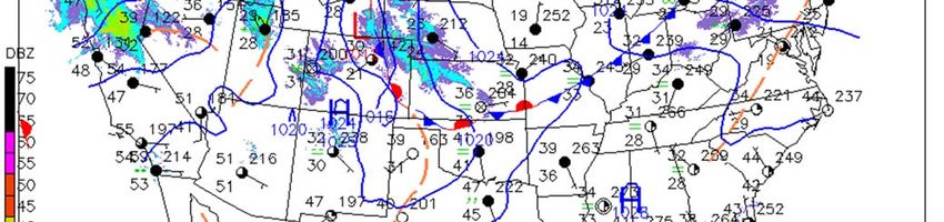
Figure 1 (“Pressures” map) was acquired from the Realtime Weather Portal and show reports of
surface air pressures (corrected to sea level) rounded to the nearest whole millibar on 16 January
2019 at 14Z. [UTC, or Z time, is five hours “ahead” of Eastern Standard Time (EST), so the 14Z
map of January 16th depicts conditions at local times of 9 AM EST (8 AM CST, 7 AM MST, 6
AM PST, etc.)].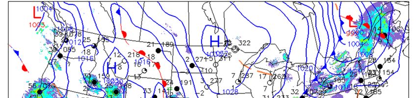
CWS1 - 2 – SP19

       Figure 1. Map of surface atmospheric pressure (reduced to sea level) at selected stations
             at 14Z 16 January 2019. [It is recommended that you print out and analyze a full-
             size copy of this figure, click here.]

Most weather map products from the RealTime Weather Portal are created by the National
Weather Service’s (NWS) National Centers for Environmental Prediction at the National
Oceanic and Atmospheric Administration (NOAA) as noted in the lower image margin
(“NCEP/NWS/NOAA”).

1. The highest plotted air pressures observation on the map of 1032 mb were located in the state
   of ________.

    a. Georgia
    b. Louisiana
c. Minnesota
d. Maine

2. The lowest reported pressure was ________ mb occurring in both states of Oregon and
   California.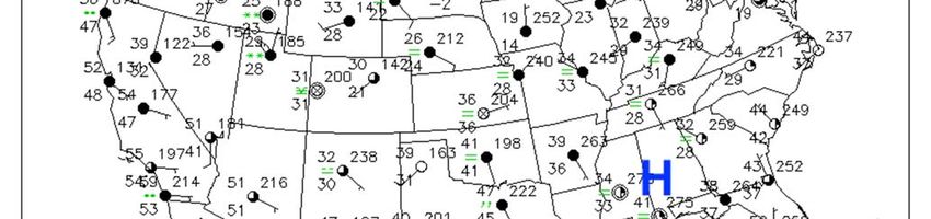
CWS1 - 3 – SP19

   a. 1004
   b. 1007
   c. 1012
   d. 1016

3. The isobars in the conventional series that will be needed to complete the pressure analysis
   between the lowest and highest values on this map are ________ mb.

   a. 998, 1002, 1006, 1010, 1014. 1018
   b. 999, 1003, 1007, 1011, 1015, 1019
   c. 1008, 1012, 1016, 1020, 1024, 1028
   d. 1013, 1018, 1023, 1028, 1031, 1036

Using a pencil on your printout, follow the steps below to complete the pressure analysis for the
map area to determine the pressure pattern that existed at the time the observations were made.
For completing the map, refer to the Tips on Drawing Isobars in the first portion of
Investigation 1A from the Investigations Manual. More than one isobar of the same value may
need to be drawn on the map if pressure values located in separate sections of the map area
require it. Consider each pressure value to be located at the center of the reported number.
Isobars with values of 1024 and 1028 mb have already been drawn on the U.S. area. Note that
labels for isobars have been added at their ends where they reached the boundary of the map area
having plotted data. For closed isobar references in a circle, that numeric denotation is placed in
the line itself.

As the course proceeds, mention of locally understood geographic regions will appear in the
Daily Weather Summaries and Current Studies. Common NWS terminology for these regions of
the country which may be useful to understanding is at:
http://www.wpc.ncep.noaa.gov/images/us_bndrys1_print.gif and
http://www.wpc.ncep.noaa.gov/images/us_bndrys2_print.gif.

4. In the state of South Dakota, there are two isobars crossing the state. The isobar bisecting the
   western part of the state near Rapid City, SD is a 1024-isobar line generally running north-
   south. One other isobar line is noted through the eastern part of the state. Given the 4-
   millibar interval convention, these two lines will separate values where the lower value on
   the map remains to one side while higher values are on the other side. The pressure values of
   locations generally east of Rapid City are therefore ________ 1024 mb.

   a. less than
   b. equal to
   c. greater than

Continue drawing and labeling isobars of the series where they existed within the data pattern
over the eastern half of the U.S. and in the western half as well. After completing all the isobars,
label the positions with the lowest value in the U.S. mid-section with bold Ls (about 1 cm high).
Label the highest pressure in the western U.S. with an H.
CWS1 - 4 – SP19

Figure 2 is the analyzed surface pressure map from the Realtime Weather Portal produced at the
NOAA’s National Centers for Environmental Prediction for 14Z 16 JAN 2019. The Figure 2
map shows the locations of isobars, air pressure system centers, and fronts at the same time as
those on the Figure 1 map you have analyzed.

          Figure 2. Analyzed NCEP surface weather map for 14Z 16 January 2019 with
              isobars, pressure systems, and precipitation.

5. The overall isobar patterns on the two maps over the coterminous U.S., particularly for the
   north central U.S. High and the Pacific Northwest Low, are generally ________. Also,
   included are shadings for precipitation occurrences around the country, based on radar
   reports.

   a. very different
   b. similar

The Figure 2 map of isobars was constructed by a computer model, based on a much more
complete set of pressure values than those shown on Figure 1. This degree of detail can be seen,
for example, on the latest surface map available, at http://www.wpc.ncep.noaa.gov/html/sfc-
zoom.php. (This may account for some of the variations between your analysis and that by the
CWS1 - 5 – SP19
computer. The computer-based analysis is the source of some additional plotted Hs denoting
local marginally higher-pressure centers and Ls for lower pressure centers, respectively.)
By analyzing the pressure values reported on weather maps to find pressure patterns, one can
locate the centers of locally highest and lowest pressures. We will see that these pressure centers
often mark the midpoints of major weather systems; either regions of fair weather or stormy
conditions, respectively.
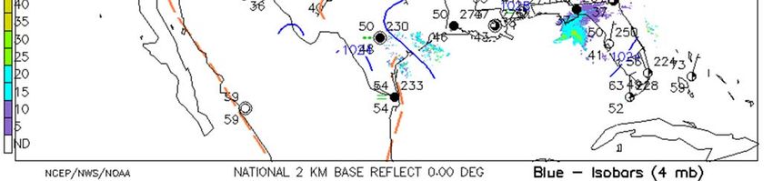
Figure 3. Un-analyzed NCEP surface weather map for 14Z 16 January 2019 with
station model plots conveying surface weather observations of temperature,
moisture, pressure, cloud cover, wind speed and direction. The centers of major
features of high and low-pressure systems are depicted with ‘H’ and ‘L’
respectively.
Figure 3 is the “U.S. - Data” map from the RealTime Weather Portal, Surface Maps, for 14Z 16
JAN 2019. It depicts weather conditions at individual locations across the contiguous U.S.
plotted using a coded format called the “surface station model.” This station model will be
examined in more detail in Investigation 2A.
6. Selected weather-reporting stations are shown on the map as circles. The wind directions at
those reporting stations are shown by the line (which can be thought of as an arrow shaft)CWS1 - 6 – SP19 depicting the air flow into each circle location that is reporting wind. In meteorology, wind at a station is identified by the direction from which the air is flowing, (i.e., air arriving at the station from the south is called a south wind). Therefore, the wind direction at Nashville, in central Tennessee, at map time was generally from the ________. [Keep in mind, because of the map projection used, the north direction may not be precisely at the top of the map. In the Chicago area, a north/south line would be nearly parallel to the Illinois-Indiana straight-line border segment.] a. north b. south c. east d. west 7. Knowing the direction from which the wind at Nashville was blowing, it would be reported as a ________ wind. a. north b. sout* c. east d. west Topic in greater depth: One knot (1 nautical mile per hour) is about 1.2 land (statute) miles per hour. The wind speed is reported by a combination of long (10 knots) and short (5 knots) “feathers” attached to the direction shaft. At map time, Nashville had a 5-knot wind (one short feather). A double circle without a direction shaft, such as seen in Mississippi & Alabama, signifies calm conditions. A shaft plotted without feathers would denote 1-2 knots. 8. Two bold blue “H”s have already been marked on the map in both North Dakota/Minnesota as well as the southern Gulf States to denote the general center of high pressure in that area. Compare the hand-twist model of a High to the wind directions at stations in the several-state area surrounding the high-pressure center. Wind directions at these stations suggest that, as seen from above, the air was circulating generally ________ around this Northern Hemisphere high-pressure center. a. counterclockwise b. clockwise 9. The winds at stations in the several-state area around the high-pressure center indicated that the air also was spiraling generally ________ the high-pressure center. a. outward from b. inward toward
CWS1 - 7 – SP19

10. This wind flow pattern about the High is therefore ________ the hand-twist model of a High.
    [Refer to Investigation 1B in the AMS Weather Studies Investigations Manual for the hand-
    twist models of Lows and Highs.]

   a. consistent with
   b. contrary to

In addition to the forcings of large-scale pressure patterns in this western portion of the country,
air flows are also greatly influenced by the mountainous, high-elevation terrain that stretches
from western Montana and Idaho southeastward to New Mexico and western Texas. As such,
wind flow patterns around the high-pressure system may not fully display the anticipated
rotational directions.

When the current weather map available on the RealTime Weather Portal shows centers of Lows
or Highs near your location, you might consider your local wind direction (as reported on
weathercasts or shown by a nearby flag flapping in the wind, for example) with map circulations
and the hand-twist models of weather systems. The typical designation of the L’s and H’s as
centers of stormy and fair-weather systems, respectively, can be compared to satellite views
showing clouds across the U.S.. Check to see if the region around a Low center is generally
cloudy or the broad area centered on a High as mostly clear. This topic will be visited more in
future Current Weather Studies.

A website that dynamically displays the forecasted wind flow at the time, shown in both
direction and speed, at locations across the U.S. can be found at: http://hint.fm/wind. Moving
your cursor across the map will give the wind speeds at specific locations. You might compare
the wind flow patterns seen at this site to those of the latest surface weather map’s positioning of
Highs and Lows. Two other interactive maps showing winds across the globe are:
http://earth.nullschool.net and http://windy.com

Further details for deciphering station data can be found in the User’s Guide (linked from the
Extras section of the RealTime Weather Portal). The reporting surface weather stations plotted
on course maps can be identified from the “Available Surface Stations” link on the Portal’s
Surface Maps data section and identities given in the User’s Guide. Also, a map of National
Weather Service (NWS) offices can be found at:
http://www.wrh.noaa.gov/wrh/forecastoffice_tab.php.

One tool for wind speed conversions between miles per hour and knots (as well as other
quantities) and their formulas can be found at: http://www.weather.gov/epz/wxcalc.

Suggestions for further activities: The Realtime Weather Portal routinely delivers unanalyzed
(“Pressures”) and analyzed (“Isobars & Pressures”) surface pressure maps. Practice drawing
isobars by calling up the unanalyzed version. Note: If you would like to practice more on
drawing isopleths (lines of a constant value) in groups of numbers, from simple to more complex
patterns, go to: http://profhorn.aos.wisc.edu/wxwise/AckermanKnox/chap1/Contour_page1.html.

Preparing for Week 2 and Beyond
CWS1 - 8 – SP19 Technology can be a useful tool to leverage and engage weather data for conceptualization and analysis. In Current Weather Studies 2, we will introduce some questions and content drawn from an ArcGIS online platform. ArcGIS online is an interactive way to map, view, and analyze spatial data such as weather observations and patterns. ESRI offers an introductory course titled “Teaching with GIS,” that presents strategies for integrating GIS to support instruction, discussion, and extended learning on any topic. Many practical ideas for GIS activities that enhance learning and critical thinking skills are shared. To help you prepare for the upcoming Current Weather Studies 2 and other Current Studies in 2019 using GIS, you are encouraged to take some time to engage in a few or all of the associated modules. Completion of the course entitles you to an ArcGIS certificate. This certificate, however, is not required for completion of this course, unless otherwise specified by your instructor or mentor. You will have to create a free account with ESRI in order to work with these modules, which only requires the use of an email address. Follow the steps on the login page and once you have completed enrollment you will be ready to begin the course at your own speed. Please visit https://www.esri.com/en-us/home to register. Locate the “Login” section on the homepage, and then choose “Create A Public Account.” After creating an account follow this link for the Training Module: https://www.esri.com/training/catalog/57630436851d31e02a43f125/teaching-with-gis:-introducti on-to-using-gis-in-the-classroom ESRI Home Website: https://www.esri.com/en-us/home ArcGIS Online Website: https://www.arcgis.com/home/index.html ©Copyright 2019, American Meteorological Society
You can also read