Synthesis of Two Degrees-of-Freedom Haptic Device
←
→
Page content transcription
If your browser does not render page correctly, please read the page content below
14th National Conference on Machines and Mechanisms (NaCoMM-09),
NIT, Durgapur, India, December 17-18, 2009                             NaCoMM-09-Paper ID XXX####

            Synthesis of Two Degrees-of-Freedom Haptic Device
                   Praveen Kumar Singh1, Subir Kumar Saha1*, and M. Manivannan2
                               1 Department of Mechanical Engineering
                      Indian Institute of Technology Delhi, New Delhi-16, India
                                 2 Department of Applied Mechanics
                       Indian Institute of Technology Madras, Chennai-36, India

                                    * Email: saha@mech.iitd.ernet.in

                                                      1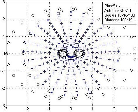
14th National Conference on Machines and Mechanisms (NaCoMM09),
NIT, Durgapur, India, December 17-18, 2009 NaCoMM-2009-###
Synthesis of Two Degrees-of-Freedom Haptic Device
Abstract This paper is organized as follows: Section 2
presents kinematic modeling, followed by the workspace
analysis in section 3. Section 4 presents the kinematic
Haptic device is a force reflecting device. In this paper,
optimization. Finally, accuracy check and conclusions
one such device is synthesized for efficient training of
are provided in sections 5 and 6, respectively.
medical students and professionals specially those re
quiring visual information of equipment and forces from
the surgeon to the microsurgical tools inserted into the
body. The device is to deliver high performance and 2 Kinematic Modeling
should be accurate. To do so, first kinematic analysis of
a suitable mechanism is performed and singularities in
its workspace were identified to form constraints for an The planar five-bar five revolute jointed parallel mech
optimization. Performance index based kinematic optim anism is shown in Figure 1. It has an end-effector point
ization of the mechanism was performed over the whole C which is connected to the base by two legs, O 1C and
workspace. The performance was then checked and lim O2C. In each of the two legs, the revolute joint connec
itations were analyzed by means of the so called force ted to the base is actuated. The mechanism is symmetric
manipulability ellipsoid. We found that the performance about Y-axis. Such a mechanism can position a point in
in terms of kinematic singularity was greatly improved X-Y plane.
for the optimized mechanism.
Keywords: Haptic devices, Kinematic singularity, Force
manipulability ellipsoid, and Performance measure.
1 Introduction
X
Haptics is the science of touch. Haptic devices can be
viewed as having two basic functions: 1) to measure po
sition and their time derivatives accurately, 2) to be able Fig. 1: Kinematic diagram
to display contact forces to the user. In this paper, a the
Let a1 , a 2 , a 3 are physical lengths of the mechan
Haptic device is synthesized to carry out virtual epidural
injection in which the tip of the needle is to be inserted ism. Then we define normalized lengths as non dimen
into the epidural space within the spinal canal surround sional parameters ri , i=1, 2, 3, i.e,
ing the spinal cord. For doing the above task, a force re
flecting simple haptic device can provide visual inform r1 = a 1 / L , r2 = a 2 / L , r3 = a 3 / L
ation and transmit force from an operator to a slave, a where, L = ( a1 + a 2 + a 3 ) / 3
slave to an operator, or in both directions, so as to give
feedback to the trainee.
Here we synthesize the mechanical part of the 2.1 Inverse Kinematics
device, based on a five-bar planar parallel mechanism.
Synthesis of such a manipulator is greatly influenced by For inverse kinematics, the location of the end-effector,
the fact that the relationship between the robot’s actuat C is given and the problem is to find the joint variables
ors and the end-effector varies with its position and dir necessary to bring the end-effector to the desired loca
ection. Only after minimizing this variation, or in other tion [1]. The position vector of the output point C in the
words maximizing the mechanical isotropy, one can reference system X-Y is given by
choose suitable actuators and design a controller. The p = ( x,y ) T
kinematic equations of mechanism describe the relation
ships between the end-effector and its actuators. The In the reference frame, the position vectors of point Bi (i
Jacobian matrix then determines the required actuator = 1, 2) can be written as
T
force/torque from a desired end-effector force/torque. b1 = ( r1 cosθ1 - r3 , r1 sinθ1 )
214th National Conference on Machines and Mechanisms (NaCoMM09),
NIT, Durgapur, India, December 17-18, 2009 NaCoMM-2009-###
and b 2 = ( r1 cosθ 2 + r3 , r1 sinθ 2 )
T and
where, θ1 and θ 2 are the actuated angles.
æ y cosθ1 - (x + r3 ) sinθ1 0 ö
Jθ = ç ÷ r1
The inverse kinematic problem can then be solved by è 0 y cosθ 2 + (r3 - x) sinθ 2 ø
writing the following constraint equations. Now, the Jacobian matrix of the five-bar mechanism is
2
( x - r1 cosθ1 + r3 ) + ( y - r1 sinθ1 ) = r2
2 2 given by
(1) -1
2 2 2
J = Jθ J p (8)
( x - r1 cosθ 2 - r3 ) + ( y - r1 sinθ 2 ) = r2
(2)
In eqs. (1) and (2), the inputs to reach the position p(x,
y) is desired based on the position of point C, obtained. 2.4 Singularity Analysis
Four solutions are achieved for the inverse kinematic
problem. Due to the existence of two Jacobian matrices, the
mechanism is said to be at a singular configuration when
2.2 Forward Kinematics either J p or J θ or both are singular. Singularity leads to
an instantaneous change of the mechanisms DoF.
The forward kinematics problem is to obtain the output
C with respect to a set of given inputs, θ1 and θ2. From 2.4.1 Inverse Kinematic Singularities
eqs (1) and (2), one obtains
x 2 + y2 - 2 ( r1 cosθ1 - r3 ) x - 2 r1 sinθ1 y - 2 r1 r3 cosθ1 This singularity occurs when the output point reaches its
limit or its boundary of the workspace. They are given
+ r32 + r12 - r22 = 0
below:
(3) At,
x 2 + y2 - 2 ( r1 cosθ2 + r3 ) x - 2 r1 sinθ2 y + 2 r1 r3 cosθ2
x = ( r1 + r2 ) cosθ1 - r3 and y = ( r1 + r2 ) sinθ1 (9)
+ r32 + r12 - r22 = 0
or, x = ( r1 + r2 ) cosθ 2 + r3 and y = ( r1 + r2 ) sinθ 2
(4)
Subtracting eq. (4) from (3), gives (10)
x=dy+e (5) and
where, x = ( r1 - r2 ) cosθ1 - r3 and y = ( r1 - r2 ) sinθ1
(11)
d = r1 ( sinθ1 - sinθ 2 ) / ( 2 r3 + r1 cosθ 2 - r1 cosθ1 ) or, x = ( r1- r2 ) cosθ2 + r3 and y = ( r1- r2 ) sinθ 2 (12)
· ·
e = r1 r3 ( cosθ1 + cosθ 2 ) / ( 2 r3 + r1 cosθ 2 - r1 cosθ1 ) There exists some non-zero θ that results in zero p
Substituting eq. (5) to eq. (3) yields vector. Infinitesimal motion of the end-effector along
2
fy +gy+h=0 (6) certain directions cannot be accomplished. Hence ma
nipulator loses one DoF. Under above singularities the
in which,
links are either fully extended or folded. Hence they are
f = 1 + d , g = 2 ( d e - d r1 cosθ1 + d r3 - r1 sinθ1 )
2
also called boundary singularities, which are shown in
2
h = e - 2 e ( r1 cosθ1 - r3 ) - 2 r1 r3 cosθ1 + r3 + r1 - r2
2 2 2 Fig. 2.
From eq. (6), two solutions for the forward kinematic
problem are obtained.
2.3 Jacobian Matrix
Let the actuated joint variables be denoted by a vector θ
and the location of the moving platform be described by
a vector p. Then the kinematic constraints imposed by
the limbs can be written in the general form as
f (p,θ) =0
Fig. 2: Boundary singularities
i.e., eqs. (1) and (2)
Differentiating eqs. (1) and (2) with respect to time, we
obtain a relationship between the input joint rates and 2.4.2 Direct Kinematic Singularities
the end-effector output velocity as
· ·
A direct kinematic singularity occurs when the determ
J pθ p =J θ (7) inant of Jp is equal to zero.
i.e, i.e., Det (Jp) =0.
The above happens
æ x - r1 cosθ1 + r3 y - r1 sinθ1 ö 1) when,
Jp = ç ÷
è x - r1 cosθ 2 - r3 y - r1 sinθ 2 ø
314th National Conference on Machines and Mechanisms (NaCoMM09),
NIT, Durgapur, India, December 17-18, 2009 NaCoMM-2009-###
r1 sinθ1 = r1 sinθ 2 care with the above mentioned checks.
and r1 cosθ1 - r3 = r1 cosθ 2 + r3
i.e. when B1 and B2 points coincide.
This singular configuration is shown Fig. 3(a). Locus of 3 Workspace Analysis
the end-effector in this case of above singularity is ob
tained as Workspace of the planar mechanism, Fig. 1 is defined as
2
x + (y -
2 2 2
r1 - r3 ) =
2
r2 the space that its end-effector can reach. A dexterous
workspace is the space within which every point can be
2
and x + (y +
2 2 2
r1 - r3 ) = r2
2 reached by the end-effector from all possible orienta
tions. Boundary singularities describe the boundary of
the workspace beyond which the end-effector cannot
2) when, reach. Equations (9-12) are actually annulus regions
x = ( r1 /2 ) ( cosθ1 + cosθ 2 ) within which the workspace lies. As there exist singular
loci inside the theoretical workspace the manipulator
y = ( r1 /2 ) ( sinθ1 + sinθ 2 ) may pass through them. Hence, there is a need to define
i.e. when point B1 C B2 lie on a straight line which is a measure of proximity to those singular loci and then
shown in Fig. 3(b). accordingly define dexterous workspace.
3.1 Condition Number: Measure of Singu
larity Proximity and Accuracy
The condition number of the Jacobian matrix can be
defined as [1]:
C = σ max /σ min
(a) (b) where s max , and s min are the largest and the smallest
Fig. 3: Direct kinematic singularity singular values of the Jacobian matrix, J, respectively.
These singular values are equal to the square root of the
In direct kinematic singularities, there exist some maximum and minimum eigenvalues of JJ T where J is
· ·
nonzero p vectors that result in zero θ vectors. That is, the Jacobian matrix. Note that the condition number of a
matrix measures the sensitivity of the solution of a sys
the end-effector can have infinitesimal motion in some
tem of linear equations to errors in data. It gives an in
directions while all actuators are completely locked.
dication of the accuracy of results from matrix inversion
Hence end-effector gains one-DOF.
and the linear equation solution. Condition number close
to one indicates a well conditioned matrix. The condi
2.4.3 Conditions for Removing Singularities tion number is independent of the scale of a manipulat
or.
In order to avoid the singularities following conditions To check accuracy we confirm end-effector velocity
are obtained. vector on a unit circle,
a) If r3 > r1 , B1 B2 will never coincide. .T .
p p =1
b) If r2 > ( r1 + r3 )
and compare the joint rates as
.T .
q JT J q = 1
The above equation represents an ellipse in joint space.
The eigen vectors of JJ T are orthogonal and the princip
al axis coincide with them. The lengths of the principal
Fig. 4: Combined singularity axis are equal to the reciprocals of the square roots of
the eigenvalues of JJ T [2]. Here, the condition number
B1 C B2 will never lie in a straight line.
is used for two different purposes: first, as a measure of
c) If r3 < ( r1 + r2 ) combined singularity is removed proximity to singularity; second, as a measure of kin
when O1 B1 C B2 O2 will never lie in a straight line. ematic accuracy.
d) If r2 ¹ r3 combined singularity is also removed, i.e., Using the Inverse kinematics algorithm, position of the
end-effector is checked for
e) r1 + r2 + r3 = 3, and 0 < r1 < 3, 0 < r2 < 3, r3 < 1.5 1. Solution exists in the joint space or not.
Rest of the combined singularity conditions are taken 2. The condition number of the Jacobian matrix.
414th National Conference on Machines and Mechanisms (NaCoMM09),
NIT, Durgapur, India, December 17-18, 2009 NaCoMM-2009-###
Using the following steps: sidering the following:
a. Workspace under boundary singularity is di 1. Condition number of the Jacobian matrix should
vided in a set of circular arcs. rise as smoothly as possible.
b. Each point on a circular arc is checked whether 2. Condition number should be low at boundaries.
solution exists or not in joint space using in 3. Workspace should be more keeping the size of
verse kinematics. device under certain limit.
c. Then at each point condition number of Jacobi Hence, we choose number of workspace points at
an matrix condition number (K) is checked and which condition number is more than 5 as performance
accordingly given a sign as measure for optimization.
Plus: if K14th National Conference on Machines and Mechanisms (NaCoMM09),
NIT, Durgapur, India, December 17-18, 2009 NaCoMM-2009-###
In order to find other two link lengths i.e. a1 and a2 f f
T
£ 1
“Points with K> 5” is checked against the workspace
measure (rMIC) for ranges of a1 and a2 given in Table 1. It is the ellipse defined by
T T -1
τ (JJ ) τ £ 1
4.1 Results Also
·
T ·
Variation of prerformance measure with fixed link length(a3)
p p =1
60
which is compared with joint rates as
·
T ·
50
T
q J J q =1
Points with condition no. > 5.
40
Above equation represents an ellipse in joint space.
30
Note that the matrices (JJ T )-1 and JJ T have same
20
eigenvectors, and that the eigenvalues of (JJ T ) -1 are the
10
reciprocals of the eigenvalues of JJ T . In other words, the
0 principal axes of the velocity and force ellipsoids coin
2 2.5 3 3.5 4 4.5 5 5.5 6 6.5 cide, and the lengths of the axes are in inverse propor
Fixed link length (a3)
tion [3]. This ellipse show how efficiently motion/force
Fig. 6: Variation of performance parameter with base can be applied in each direction. We see the effect of
length. variation of condition number on force/torque trans
formation between end-effector and joint space through
an example.
Fig. 6: Force/Torque Transformation
Fig. 8 shows different sizes and shapes of torque ellipses
Fig. 7: Graph showing Performance parameter variation
that occur at three different positions of the mechanism.
with radius of MIC
The ellipses at y=3 and y= 18 have different shapes, i.e.,
the condition number at y= 3 are an average of 1.5 times
From Fig. 7 we can see that “Points with K>5” are min larger than those at y=18. In other words it has over one
imum corresponding two architectures, i.e. at and a half times the average force capabilities in the
a1 = 9; a 2 = 14; a 3 = 3 ; and a1 = 10; a 2 = 15; a 3 = 3 . centre of its workspace than it does at the edges of its
Since, for latter workspace is higher we choose it as our workspace.
final design.
5 Accuracy
A force ellipsoid is used for describing the force trans
mission characteristics of a manipulator at a given pos
ture. Forces in joint space and task space are mapped via
Jacobian through the relation.
T
τ=J f (13)
Where f is the force vector in task space and τ is the
joint torque vector. Using Eq. 13, we obtain
T T T -1
f f = τ (JJ ) τ
To check the accuracy we confirm the end-effector force
vector on a unit circle, i.e.,
614th National Conference on Machines and Mechanisms (NaCoMM09),
NIT, Durgapur, India, December 17-18, 2009 NaCoMM-2009-###
Acknowledgment
This work is supported under IIT Delhi - IIT Madras
collaborating project entitled “Development of 2D
Haptic Device for Virtual Reality Based Medical Simu
lation with Haptic Feedback” sponsored by DST, Govt.
of India. We take this opportunity to thank all members
of Mechatronics Lab, IIT Delhi and Haptics lab, IIT
Madras for their supports. Special thanks to Ph.D stu
dent Mr. Suril Shah for his help during the work of first
author whose outcome is this paper.
References
[1] L. Tsai, Robot analysis: The mechanics of serial
and parallel manipulators, Wiley & Sons Inc., New
York,
1999.
Fig. 5: Graph showing Force/Torque ellipses over the
workspace for selected configuration. [2] J. O. Kim, P.K. Khosla, “Dexterity Measures for
Design and Control of Manipulators”, Proc. IROS ‘91,
IEEE/RSJ Int. Workshop Intell. Robots & Sys. (Osaka,
Fig. 9 shows the relative sizes of force torque el
Japan), Nov. 3-5, 1991.
lipses over the workspace for selected configuration,
which is used to check the performance of the proposed [3] S. Chiu, "Task compatibility of manipulator pos
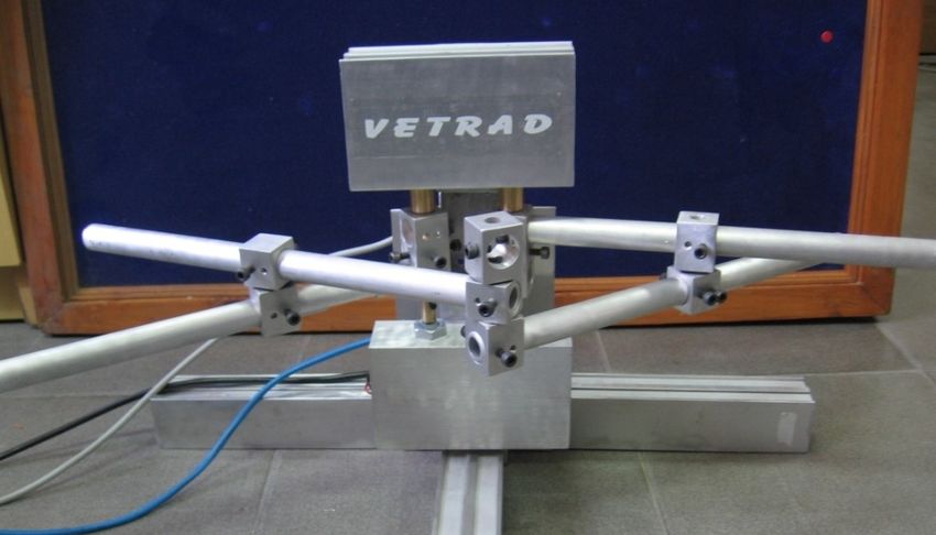
design. Fig. 10 shows the photograph of a real prototype tures," Int. J. of Robtics Research, 1990.
made.
Fig. 10: Prototype of synthesized mechanism
6 Conclusions
A two degrees-of-freedom haptic device is synthesized
using a systematic approach. The device has improved
performance characteristics which are also analytically
analyzed. Based on the above synthesis a prototype of
the device was developed, which functioned appropri
ately. However, further testing is required after interfa
cing with a virtual environment. This will be taken up in
future.
7You can also read