Targeting Constant Money Growth at the Zero Lower Bound
←
→
Page content transcription
If your browser does not render page correctly, please read the page content below
Targeting Constant Money Growth
              at the Zero Lower Bound∗

            Michael T. Belongiaa and Peter N. Irelandb
                           a
                               University of Mississippi
                                  b
                                    Boston College

          Unconventional policy actions, including quantitative eas-
      ing and forward guidance, taken during and since the finan-
      cial crisis and Great Recession of 2007–09, allowed the Federal
      Reserve to influence long-term interest rates even after the
      federal funds rate hit its zero lower bound. Alternatively, sim-
      ilar policy actions could have been directed at stabilizing the
      growth rate of a monetary aggregate in the face of severe
      disruptions to the financial sector and the economy at large.
      A structural vector autoregression suggests it would have been
      feasible for the Fed to target the growth rate of a Divisia mon-
      etary aggregate once the federal funds rate had reached its
      zero lower bound and that doing so would have supported a
      stronger, more rapid recovery.
      JEL Codes: E21, E32, E37, E41, E43, E47, E51, E52, E65.

1.   Introduction

The financial crisis and Great Recession of 2007–09 seemingly
required major changes in Federal Reserve (Fed) operating proce-
dures. Pre-crisis, the Fed conducted monetary policy by targeting
the interest rate on overnight, interbank loans: the federal funds
rate. When the Fed wished to tighten monetary policy, it raised
its target for the federal funds rate; conversely, when it wished to

    ∗
      We would like to thank John Taylor, John Williams, and two anonymous
referees for extremely helpful comments on previous drafts of this paper. Nei-
ther of us has received any external support for, or has any financial interest that
relates to, the research described in this paper. Author contact: Belongia: Univer-
sity of Mississippi, Box 1848, University, MS 38677; e-mail: mvpt@earthlink.net.
Ireland: Boston College, 140 Commonwealth Avenue, Chestnut Hill, MA 02467;
e-mail: peter.ireland@bc.edu.

                                         159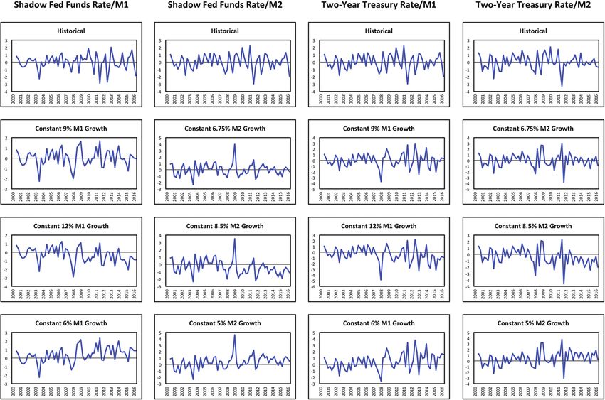
160          International Journal of Central Banking                March 2018

ease, it lowered its funds rate target. After the target was reduced
to a range of 0 to 0.25 percent in December 2008, however, the zero
lower bound (ZLB) on the federal funds rate forced the Fed to look
for other ways of providing additional monetary stimulus to help
output and employment recover and prevent inflation from falling
further.
    Bernanke (2012) describes two sets of tools that the Fed adopted,
under his Chairmanship, to continue pursuing these goals. Multiple
waves of large-scale asset purchases of U.S. Treasury bonds and gov-
ernment agency mortgage-backed securities, known more popularly
as “quantitative easing” or “QE,” aimed to put direct downward
pressure on long-term interest rates. Meanwhile, “forward guid-
ance,” in the form of official policy statements, promised to keep
short-term interest rates low for an extended period of time, even
as the economy began to recover. These public statements were
intended to reduce long-term rates further by working on the yield
curve through expectational channels. Although these tactics kept
the focus of Federal Reserve policy squarely on interest rates, the
severity of the downturn caused the Fed’s interventions in bond mar-
kets to grow enormously in size and scope while its communication
strategy evolved into a program vastly more ambitious and complex
than originally conceived.1
    Viewed from a different angle, however, there may be less to
distinguish between monetary policy before and after the crisis. This
is because, in more normal times, any increase in the Fed’s target
for the federal funds rate still required open market operations that
drained reserves from the banking system. This decrease in reserves
worked through textbook channels to slow the growth rate of money
and thereby dampened economic activity generally and slowed infla-
tion specifically. Likewise, when the Fed lowered its target for the

   1
     Bernanke, Reinhart, and Sack (2004) discuss alternative monetary policy
strategies once the zero lower bound constraint binds. Written before the Great
Recession, these options were examined because, under sustained low inflation,
the zero lower bound was becoming more than a theoretical curiosity. One of the
suggested strategies was to stimulate economic activity by increasing the size and
altering the composition of the Federal Reserve’s balance sheet in a manner that
would raise asset values and reduce yields. The authors, however, do not consider
the potential effects of changes in the quantity of money.
Vol. 14 No. 2              Targeting Constant Money Growth                    161

funds rate, it engineered the desired fall through open market oper-
ations that increased the supply of reserves, which caused broad
money growth to accelerate with more rapid economic activity and
inflation to follow. From this viewpoint, large-scale asset purchases
might have worked mainly to increase the quantity of reserves sup-
plied to the banking system, leading to faster money growth, higher
output, and more stable inflation.2 Forward guidance might have
worked, as well, to convince the public that open market operations
designed to stimulate broad money growth would continue even after
the economy began to recover; working again through expectational
channels, this more persistent increase in money growth might have
contributed to a stronger economy right away. Taking a similar view,
Taylor (2009) argues that the Federal Reserve might have conducted
monetary policy in a more systematic fashion by switching to a ver-
sion of Friedman’s (1960) k-percent rule for constant money growth
after the federal funds rate hit its zero bound in 2008.
    If the monetary policy strategies available to the Fed before and
after the recent financial crisis are similar in principle if not degree,
it seems reasonable to ask whether the Fed could have responded to
the economic downturn of 2007–09 by adopting a constant rate of
money growth as an intermediate target rather than continuing to
focus on interest rates. Moreover, if an alternative intermediate tar-
get of constant money growth had been chosen to guide the course
of monetary policy, it must be asked whether that strategy would
have made the U.S. economy’s recovery from the Great Recession
stronger or more rapid.
    This paper investigates both questions by modifying the struc-
tural vector autoregression (SVAR) developed in Belongia and
Ireland (2015, 2016b). Importantly, the SVAR brings data on both
interest rates and money growth to bear in gauging the stance and
consequences of Federal Reserve policy before, during, and since the
financial crisis and Great Recession. The paper uses this model to

    2
      See Orphanides and Wieland (2000) for an early theoretical treatment of the
zero lower bound, motivated by the Japanese experience of the 1990s, that is
consistent with this view. In their model, the central bank uses its influence over
the monetary base to manage the federal funds rate during normal times, while
targeting the monetary base even more aggressively to continue pursuing its sta-
bilization goals in exceptional circumstances where short-term interest rates are
constrained by the zero lower bound.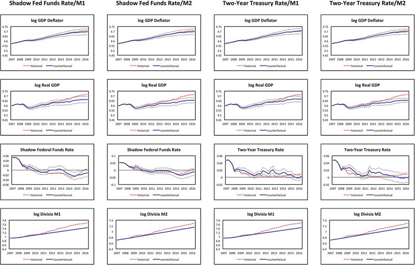
162          International Journal of Central Banking              March 2018

consider a range of counterfactual scenarios in which the Federal
Reserve succeeds in maintaining a constant rate of broad money
growth while its funds rate target is up against the zero lower
bound.3 Reassuringly, interest rates are often higher along their
counterfactual paths than they were historically, suggesting that
these alternative paths for money would have been feasible in prac-
tice. Indeed, in light of these counterfactual simulations, the per-
sistence of extremely low interest rates after the end of the Great
Recession could be seen as a consequence not of a dramatically
expansionary monetary policy but, instead, of insufficiently accom-
modative rates of money growth. The declining velocities of the mon-
etary aggregates observed during and since the financial crisis also
play a role in shaping the results, which highlight the importance of
maintaining robust rates of monetary expansion in the face of severe
disruptions to the financial system and economic activity as a whole.
Overall, the results provide evidence that the Fed could have suc-
cessfully directed its efforts towards stabilizing money growth while
the funds rate remained at its zero lower bound and, in so doing,
generated more favorable economic outcomes.

2.    Money, Output, and Prices Before, During,
      and Since the Crisis: An Overview

Before describing the model and presenting the results, this section
provides an overview of the behavior of the monetary aggregates over
the period from 2000 through 2016 and summarizes the reduced-
form relationships between these measures of money and real GDP
and the GDP deflator as indexes of aggregate output and prices.
To begin, the two panels on the left-hand side of figure 1 plot year-
over-year growth rates of the Divisia M1 and M2 monetary aggre-
gates used throughout this study. The assets included in Divisia

   3
     This analysis is therefore in much the same spirit of McCallum (1990), who
examined whether a rule for growth in the monetary base could have prevented
the Great Depression, and Bordo, Choudhri, and Schwartz (1995), who simu-
lated the potential effects on output and inflation during the Depression under
two variants of Friedman’s k-percent rule. Although these studies show effects on
nominal income or prices and output separately that are of different magnitudes,
both suggest that economic performance under a money growth rule would have
been substantially better than that depicted by the actual data.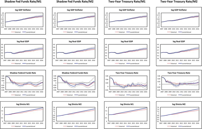
Vol. 14 No. 2             Targeting Constant Money Growth                   163

        Figure 1. Divisia Money Growth and Velocity

Notes: Panels on the left show year-over-year growth rates of the Divisia mone-
tary aggregates, with periods of quantitative easing shaded. Panels on the right
show the income velocities of the Divisia monetary aggregates.

M1 and M2 are the same as those in the Federal Reserve’s offi-
cial, simple-sum M1 and M2 measures of money. Both measures of
Divisia money are compiled, however, using the economic aggrega-
tion techniques first outlined by Barnett (1980) and reviewed more
recently in Barnett (2012). These techniques allow the Divisia mon-
etary aggregates to accurately track the true flows of monetary
services generated by their constituent assets, most of which pay
interest at different rates. It accomplishes this in much the same
way that more familiar macroeconomic quantity aggregates, such as
real GDP, measure service flows generated by different goods and
services based on the prices that demanders are willing to pay for
those products. The Divisia monetary aggregates correct, as well,
for distortions in the Federal Reserve’s official monetary aggregates
induced by the proliferation of deposit sweep programs, described by
Cynamon, Dutkowsky, and Jones (2006). Prior to the financial crisis,
these programs allowed banks to reduce their holdings of required
reserves without changing the public’s perception of the amount of
funds held on deposit at those banks. Barnett et al. (2013) describe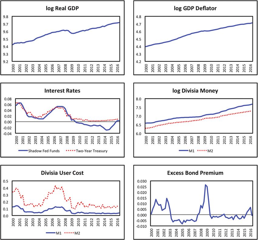
164        International Journal of Central Banking        March 2018

the construction of these Divisia monetary aggregates in full detail;
the series themselves are available through the Center for Financial
Stability’s website.
    The shaded portions of each panel on the left-hand side of
figure 1 identify periods during which the Federal Reserve conducted
its three waves of quantitative easing, operations that increased
the Federal Reserve Bank of St. Louis’s adjusted monetary base
from $872 billion in August 2008 to $4,097 billion in August 2014.
However, as the figure clearly shows, quantitative easing did not
generate the same kind of explosive growth in broader measures of
money. One reason for the disparate effects of large-scale asset pur-
chases on the monetary base relative to broad monetary aggregates
is the Federal Reserve’s decision to begin paying interest on reserves.
Ireland (2014) shows that the ability to pay interest on reserves gives
the central bank a second instrument of monetary policy, one that
works to shift the demand curve, rather than the supply curve, in the
market for reserves. In particular, for any given level of the federal
funds rate, movements from an initial equilibrium in which inter-
est is not paid on reserves to a new equilibrium in which interest
is paid on reserves at a rate that is very close to the target federal
funds rate itself triggers a potentially large rightward shift in the
demand curve for reserves. If the central bank then accommodates
this increase in demand with an equally large increase in the supply
of reserves, the monetary base can be expanded without generating
additional broad money growth or inflation. Indeed, an increase in
banks’ holdings of excess reserves of close to $2,700 billion accounts
for about 84 percent of the increase in the adjusted monetary base
between 2008 and 2014. Thus, it appears that to a large extent,
quantitative easing simply accommodated the increased demand for
reserves brought about by the Fed’s new interest-on-reserves policy.
Put another way, it seems that the Fed intentionally used interest
on reserves to “sterilize” much of the increase in the base generated
by quantitative easing.
    Even though much of the effect of quantitative easing appears
to have been absorbed by holdings of excess reserves, the left-hand
panels of figure 1 also make clear that QE did have at least some
expansionary effects on broader measures of money. Moving from
the first half of the sample from 2000 through 2007 to the second
half running from 2008 through the second quarter of 2016, average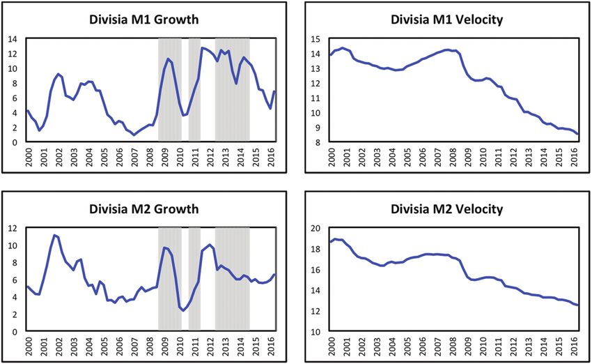
Vol. 14 No. 2            Targeting Constant Money Growth                165

annual Divisia M1 growth increases from about 4.5 to 9 percent,
while average annual Divisia M2 growth increases from slightly less
than 6 to 6.75 percent. Nevertheless, whatever effects QE had on
average rates of broad money growth, the pattern of money growth
appears, overall, to have been “consistently inconsistent.” Measured
by either of the Divisia aggregates, money growth rose and then fell
during QE1, accelerated throughout QE2, and finally drifted lower
during much of QE3. The two panels on the right-hand side of figure
1, meanwhile, show that the downward trend in the income velocity
of the Fed’s official, simple-sum M2 measure studied by Anderson,
Bordo, and Duca (2016) also appears in the velocities of the Divisia
aggregates. This downward trend in velocity continues even after
short-term interest rates reached their lower bound in 2008, a pat-
tern consistent with Anderson, Bordo, and Duca’s (2016) argument
that flight-to-quality dynamics during and since the financial crisis
increased the public’s demand for the safe and liquid assets included
in M1 and M2.
    The implication of this first set of graphs is that Fed policy suc-
ceeded only partially in supporting the monetary system against
the severe disruptions set off by the financial crisis of 2007–08 and
the sharp downturn in aggregate economic activity that followed.
Although the money supply did not fall during the Great Recession
as Friedman and Schwartz (1963) show that it did during the Great
Depression, the payment of interest on reserves appears to have
impeded multiple waves of QE from generating consistent growth
in broad monetary aggregates.4 Any expansionary effects of quan-
titative easing were dampened further by a decline in velocity that
called for even higher rates of money growth to stabilize nominal
income and spending. Whatever indications of monetary ease were
given by persistently low values of the funds rate or flattening of the
yield curve, the data for money growth indicate a restrictive policy
stance throughout much of the post-crisis period.
    If the observed monetary growth rates are suggestive of pol-
icy actions that were insufficiently accommodative, it still is pos-
sible that more strenuous efforts to increase the growth rates of the
broad monetary aggregates only would have led to further declines in

  4
   See Currie (1934) for a much earlier analysis that emphasizes many of the
same points made by Friedman and Schwartz (1963).
166 International Journal of Central Banking March 2018
velocity, without noticeable effects on aggregate output and prices.
The statistics in table 1, however, provide evidence to the contrary.
This table reports correlations between real GDP, the GDP defla-
tor, and each measure of money after the logarithms of all series
are passed through the filter developed by Baxter and King (1999)
to isolate fluctuations occurring at business-cycle frequencies corre-
sponding to periods between eight and thirty-two quarters. These
tables show that, in fact, modest correlations between money, out-
put, and prices seen over an extended sample of quarterly data run-
ning from 1967:Q1 through 2016:Q2 become much stronger when
recomputed using the data from 2000:Q1 through 2016:Q2 that are
the principal focus here. The peak correlation between Divisia M1
and real GDP rises from 0.32 for the longer sample to 0.73 for the
period since 2000; the strongest correlation between Divisia M1 and
the deflator rises from 0.38 for the full sample to 0.77 since 2000.
Likewise, for Divisia M2, its peak correlation with real GDP rises
from 0.45 since 1967 to 0.69 since 2000, and its strongest correlation
with the GDP deflator rises from 0.67 since 1967 to 0.81 since 2000.5
Of course, these are only reduced-form statistics, yet they are, if any-
thing, consistent with the presence of stronger links between money
and economic activity during the period leading up to, during, and
since the financial crisis and Great Recession, including the seven
years during which the federal funds rate remained at its zero lower
bound.
This preliminary look at the data, therefore, leads back to the
questions that motivate this study. First, even with short-term inter-
est rates near their zero lower bound, could the Fed have gener-
ated a higher and more stable rate of growth for a broad monetary
aggregate since 2008? And, second, would the economic recovery
have been stronger or more rapid had the Fed pursued this pol-
icy option instead of one with continued focus on interest rates?
Answering these questions requires more structure to be imposed
on a wider range of data. Hence, the analysis turns next to the
structural VAR.
5
The lags at which peak correlations between money, output, and prices
can be found also lengthen when moving from the longer sample to the most
recent period. These changes in lag lengths follow broader trends documented
and discussed by Belongia and Ireland (2015, 2016b, 2017).Table 1. Correlations between the Cyclical Components of Real GDP,
the GDP Deflator, and Lagged Divisia Money
Vol. 14 No. 2
k 15 14 13 12 11 10 9 8 7 6 5 4 3 2 1 0
A. Real GDP, 1967:Q1–2016:Q2
M1 −0.20 −0.18 −0.14 −0.08 −0.02 0.04 0.11 0.17 0.22 0.27 0.31 0.32 0.31 0.28 0.21 0.13
M2 −0.35 −0.31 −0.26 −0.19 −0.11 −0.03 0.06 0.15 0.25 0.34 0.41 0.45 0.45 0.40 0.32 0.21
B. GDP Deflator, 1967:Q1–2016:Q2
M1 0.16 0.24 0.30 0.35 0.37 0.38 0.36 0.31 0.24 0.14 0.03 −0.09 −0.20 −0.30 −0.36 −0.40
M2 0.59 0.65 0.67 0.66 0.61 0.53 0.41 0.27 0.09 −0.09 −0.28 −0.44 −0.56 −0.63 −0.64 −0.61
C. Real GDP, 2000:Q1–2016:Q2
M1 0.01 0.16 0.31 0.46 0.58 0.67 0.71 0.73 0.72 0.67 0.60 0.49 0.32 0.12 −0.08 −0.22
M2 0.36 0.47 0.58 0.66 0.69 0.66 0.59 0.50 0.40 0.28 0.16 0.01 −0.16 −0.35 −0.51 −0.59
D. GDP Deflator, 2000:Q1–2016:Q2
M1 0.46 0.59 0.70 0.76 0.77 0.73 0.67 0.59 0.47 0.33 0.15 −0.03 −0.21 −0.34 −0.40 −0.39
M2 0.78 0.81 0.79 0.72 0.59 0.44 0.29 0.13 −0.04 −0.21 −0.38 −0.53 −0.62 −0.63 −0.55 −0.40
Targeting Constant Money Growth
Note: Each entry shows the correlation between the cyclical component of real GDP or the GDP deflator in quarter t and the cyclical component of
Divisia M1 or M2 in quarter t − k.
167168 International Journal of Central Banking March 2018
3. Interest Rates, Money, and Monetary Policy
in a Structural VAR
The structural vector autoregression developed in Belongia and
Ireland (2015, 2016b) describes the behavior of six variables: the
GDP deflator, real GDP, the federal funds rate, a Divisia monetary
aggregate and its associated user cost index, and a measure of com-
modity prices. Here, this model is modified and extended to address
issues raised by the financial crisis, the Great Recession, and their
aftermath, events which clearly set the more recent period apart from
earlier episodes in U.S. monetary, financial, and economic history.
The modified model estimated here retains the GDP deflator and
real GDP as its measures of aggregate prices Pt and output Yt and
uses either Divisia M1 or M2 as the measure of money Mt . To distin-
guish more sharply between the demand for and supply of money, the
model also continues to exploit information in the associated Divisia
monetary user cost index Ut as explained in more detail below.
To capture more fully the effects that the Federal Reserve’s large-
scale asset purchases and forward guidance have had on the Amer-
ican economy through traditional interest rate channels, this study
replaces the federal funds rate with either of two alternative inter-
est rate measures Rt . The first alternative, Wu and Xia’s (2016)
measure of the shadow federal funds rate, is derived from a non-
linear model that accounts for the zero lower bound on the actual
funds rate, but follows Black (1995) by using information in the
term structure of interest rates to deduce the shadow rate—which
may be negative—consistent with the behavior of longer-term bond
yields. The second is a more direct measure of intermediate-term
interest rates—the two-year U.S. Treasury yield—that, according
to Swanson and Williams (2014), continued to reflect the effects of
Federal Reserve policy actions through most of the ZLB period.6
Finally, the modified model estimated here replaces the commod-
ity price index with Gilchrist and Zakrajšek’s (2012) measure Xt
of the excess bond premium. Although the identification scheme
6
Gertler and Karadi (2015), Gilchrist, López-Salido, and Zakrajšek (2015),
and Hanson and Stein (2015) also use the two-year Treasury rate to help gauge
the effects of Federal Reserve policy during and since the financial crisis and
Great Recession.Vol. 14 No. 2 Targeting Constant Money Growth 169
outlined below makes no attempt to distinguish shocks originating
in the non-bank financial sector from other non-policy shocks affect-
ing the U.S. economy during the crisis, including this measure in the
model’s information set helps ensure that macroeconomic volatility
due to financial stress before, during, and since the crisis does not
get misattributed to monetary policy.
All variables enter the SVAR in logarithms, except for the inter-
est rate, the Divisia monetary user cost, and the excess bond pre-
mium, which enter as decimals, e.g., Rt = 0.05 or Rt = −0.01 for an
annualized shadow funds rate equal to +5 or −1 percent. Figure 2
plots all of the quarterly series. The data for real GDP, the GDP
deflator, and the two-year Treasury yield are drawn from the Federal
Reserve Bank of St. Louis’s Federal Reserve Economic Data (FRED)
database; those for the Divisia M1 and M2 quantity and user cost
aggregates are from the Center for Financial Stability’s website. The
series for the shadow federal funds rate comes from Jing Cynthia
Wu’s webpage at the University of Chicago, and that for the excess
bond premium from Simon Gilchrist’s webpage at Boston Univer-
sity. The sample of data runs from 2000:Q1 through 2016:Q2, so as
to focus on the lead-up to the financial crisis of 2007–08 and the
Great Recession and slow recovery that followed, while also provid-
ing enough observations to estimate the parameters of the SVAR
with a reasonable degree of precision.
Collecting the variables into the 6×1 vector
Zt = Pt Yt Rt Mt Ut Xt , (1)
the structural model can be written as
AZt = μ + Φ1 Zt−1 + Φ2 Zt−2 + εt , (2)
where A is a 6×6 matrix of impact coefficients, normalized to have
positive elements along its diagonal, μ is a 6×1 vector of intercept
terms, Φ1 and Φ2 are 6×6 matrices of autoregressive coefficients,
εt is a 6×1 vector of serially and mutually uncorrelated structural
shocks, normally distributed with zero means and
Eεt ε = I6 , (3)
and I6 is the 6×6 identity matrix. The short sample of data used to
estimate the model dictates the choice to place two lags of Zt on the170 International Journal of Central Banking March 2018
Figure 2. Data Used to Estimate the Vector
Autoregressions
right-hand side of (2). Multiplying (2) by A−1 leads to the reduced
form
Zt = ν + Γ1 Zt−1 + Γ2 Zt−2 + zt , (4)
where ν = A−1 μ, Γ1 = A−1 Φ1 , and Γ2 = A−1 Φ2 , and the 6×1
vector of zero mean disturbances zt = A−1 εt is such that
Ezt zt = Ω = A−1 (A−1 ) . (5)
Since the reduced-form covariance matrix Ω has only twenty-one
distinct elements, at least fifteen restrictions must be imposed on
the thirty-six elements of A in order to identify the structural dis-
turbances based on information in the data. A popular approach toVol. 14 No. 2 Targeting Constant Money Growth 171
solving this identification problem follows Sims (1980) by imposing
a lower triangular structure on A so that, suppressing the intercept
and autoregressive terms that appear in (2) to focus on the contem-
poraneous relationships between the observable variables and the
structural disturbances, the model specializes to
⎡ ⎤⎡ ⎤ ⎡ p ⎤
a11 0 0 0 0 0 Pt εt
⎢ ⎥ ⎢ Y ⎥ ⎢ εy ⎥
⎢ a21 a22 0 0 0 0 ⎥⎢ t ⎥ ⎢ t ⎥
⎢ ⎥⎢ ⎥ ⎢ mp ⎥
⎢ a 0 ⎥ ⎢ ⎥ ⎢ ⎥
⎢ 31 a32 a33 0 0 ⎥ ⎢ Rt ⎥ ⎢ εt ⎥
⎢ ⎥⎢ ⎥ = ⎢ md ⎥ . (6)
⎢ a41 a42 a43 a44 0 0 ⎥ ⎢ Mt ⎥ ⎢ ε t ⎥
⎢ ⎥⎢ ⎥ ⎢ ⎥
⎢ a ⎥⎢ ⎥ ⎢ u ⎥
⎣ 51 a52 a53 a54 a55 0 ⎦ ⎣ Ut ⎦ ⎣ εt ⎦
a61 a62 a63 a64 a65 a66 Xt εxt
With the variables ordered the same way in (6) as in (1), this
identification scheme is based partly on the assumption that mone-
tary policy shocks, measured by the third element εmp t in the vector
of structural disturbances εt , affect the aggregate price level and out-
put with a one-period lag. Leeper and Roush (2003) note, however,
that when a monetary aggregate also appears in the list of variables
used to estimate the model, as is the case here, a triangular scheme
that orders the interest rate behind prices and output but ahead
of money also reflects assumptions that distinguish money supply
from money demand. In particular, the third equation in (6) can be
interpreted as a monetary policy rule of the same general form
a31 Pt + a32 Yt + a33 Rt = εmp
t (7)
as in Taylor (1993), which describes how the Federal Reserve sets
its target for the interest rate with reference to the current period’s
values of aggregate prices and output. Under this interpretation,
the money supply then adjusts elastically so as to satisfy the fourth
equation in (6), which can be viewed as a flexibly parameterized
money demand relationship,
a41 Pt + a42 Yt + a43 Rt + a44 Mt = εmd
t , (8)
that links the nominal quantity of money demanded to the aggregate
price level and aggregate output as scale variables and the interest
rate as an opportunity cost variable.172 International Journal of Central Banking March 2018
Thus, while the lagged terms that appear implicitly in (6)–(8)
and more explicitly in (2) allow for flexible dynamics between
the lags of interest rates and money, the view of monetary pol-
icy reflected in this triangular specification resembles closely the
one taken by the canonical New Keynesian model, as depicted in
textbook presentations such as Galı́’s (2015): the Federal Reserve is
described as targeting the interest rate based on output and infla-
tion, leaving the money stock to expand or contract as needed to
fully accommodate changes in money demand.7 More generally, in
the same language of Cushman and Zha (1997), Leeper and Roush
(2003), Leeper and Zha (2003), and Sims and Zha (2006), the system
in (6) identifies the first two elements of εt as disturbances to the
sluggishly moving “production sector” of the economy and the last
two elements of εt as shocks to a more quickly adjusting “informa-
tion sector.” The triangular scheme distinguishes these shocks from
those to monetary policy and money demand, but does not assign
any specific structural interpretation to them.
Belongia and Ireland (2015, 2016b) take an alternative approach
to identifying structural shocks in systems like (2) and (3) by impos-
ing additional restrictions on the money demand relationship in
order to allow for a finite elasticity of money supply and, by exten-
sion, a richer set of interactions between interest rates and the money
stock in shaping the effects of monetary policy disturbances. This
alternative model, in the modified form used here, parameterizes A
so that (2) becomes
⎡ ⎤⎡ ⎤ ⎡ p ⎤
a11 0 0 0 0 0 Pt εt
⎢ a ⎢
0 ⎥ ⎢ Yt ⎥ ⎢ εyt ⎥
⎥ ⎥ ⎢
⎢ 21 a22 0 0 0 ⎥
⎢ ⎥⎢ ⎥ ⎢ mp ⎥
⎢ a31 a32 a33 a34 0 ⎢
0 ⎥ ⎢ Rt ⎥ ⎢ εt ⎥
⎥ ⎥ ⎢
⎢ ⎥
⎢ ⎥⎢ ⎥=⎢ ⎥ , (9)
⎢ −a44 −a44 0 a44 a45 0 ⎥ ⎢ Mt ⎥ ⎢ εmd ⎥
⎢ ⎥⎢ ⎥ ⎢ t
⎥
⎢ −a54 0 ⎥ ⎢
a53 a54 a55 0 ⎦ ⎣ Ut ⎦ ⎣ εt ⎦ ⎥ ⎢ ms ⎥
⎣
a61 a62 a63 a64 a65 a66 Xt εxt
7
See Belongia and Ireland (2016a) for further elaboration on this New Keyne-
sian interpretation of conventionally specified structural VARs, and for an explicit
Bayesian comparison between the New Keynesian benchmark and an alternative
that allows changes in the money stock to play a greater role, operating through
“classical” channels of monetary transmission.Vol. 14 No. 2 Targeting Constant Money Growth 173
again suppressing explicit reference to the intercept and autoregres-
sive terms to focus on the contemporaneous relationships between
the observable variables and the structural shocks.
The first two equations in (9) impose the same timing restrictions
used in the fully recursive, triangular model such that the aggre-
gate price level and output respond to monetary policy (and other)
shocks with a one-period lag. In defense of this timing assumption,
note from table 1 that, for the sample period running from 2000:Q1
through 2016:Q2, correlations between the cyclical components of
money and output and money and the price level are consistently
negative, a reduced-form relationship more easily explained if mon-
etary policy responds immediately to output and inflation than if
output and inflation respond immediately to monetary policy. In (9)
as in (6), therefore, εpt and εyt appear as shocks to a sluggish pro-
duction sector, identified separately from shocks to monetary policy
and money demand but not given any structural interpretation, for
example, as shocks to aggregate supply and demand.
The third equation in (9) describes a monetary policy rule more
general than (7) and takes the form
a31 Pt + a32 Yt + a33 Rt + a34 Mt = εmp
t . (10)
Following Ireland (2001), (10) can be interpreted as a generalized
Taylor (1993) rule that includes the money stock together with the
aggregate price level and output in the list of variables that Fed-
eral Reserve policymakers refer to when setting their interest rate
target. Following Leeper and Roush (2003), (10) also can be inter-
preted as a monetary policy rule that features a finite elasticity
of money supply, in contrast to the implicit assumption of infinite
money supply elasticity reflected in (7), the original Taylor (1993)
rule, and the standard New Keynesian model. Yet another interpre-
tation, supported by the reduced-form connections between money,
output, and prices shown in table 1, is that (10) captures simul-
taneous movements in the interest rate and money, both of which
are important in transmitting the effects of monetary policy shocks
through the economy.
Belongia and Ireland (2015) test the general specification in
(10) against the more constrained alternative originally proposed by
Sims (1986) and used more recently by Leeper and Roush (2003) and
Sims and Zha (2006) in which α31 = α32 = 0, so that the price level174 International Journal of Central Banking March 2018
and output are excluded from the monetary policy rule. Belongia
and Ireland (2015, 2016b) work with this simpler version of the rule
because, when using data from 1967:Q1 through 2007:Q4, imposing
these constraints does not lead to statistically significant deteriora-
tion in the model’s fit. As shown below, however, these constraints
are rejected quite decisively in data from 2000:Q1 through 2016:Q2,
reflecting mainly the Federal Reserve’s attempts to use monetary
policy to stabilize output over this most recent period. Hence, the
more flexible specification is used here. Keating et al. (2014) and
Arias, Caldara, and Rubio-Ramirez (2016) are two other papers
that experiment, successfully, in bringing information in both inter-
est rates and monetary aggregates to bear in identifying monetary
policy shocks and estimating their effects on the economy.
The fourth equation in (9) draws on economic theory to parame-
terize the money demand relationship more tightly as
a44 (Mt − Pt − Yt ) + a45 Ut = εmd
t . (11)
Relative to (8) from the triangular model, (11) follows Cush-
man and Zha (1997) by imposing a unitary price elasticity, so that
the demand for money is described explicitly as a demand for real
cash balances. Here, again modifying the specification from Belon-
gia and Ireland (2015, 2016b), a unitary income elasticity of money
demand also is imposed; though not essential for identification, this
constraint also helps distinguish between money demand and money
supply, is not rejected by the data, and is consistent with theories of
money demand that predict a stable relationship between monetary
velocity and an opportunity or user cost variable. Finally, compared
with (8), (11) replaces the interest rate Rt with the Divisia user cost
index Ut , which measures the “price” of monetary services in a the-
oretically coherent way; interest rates, by contrast, are linked to the
price of bonds as money substitutes.8 Thus, drawing on the logic
behind identification in more traditional simultaneous equation sys-
tems, (10) and (11) work to disentangle shocks to money supply from
those to money demand, first, by using quantity-theoretic restric-
tions that associate “money supply” with nominal cash balances and
“money demand” with real cash balances relative to income. These
8
See Barnett (1978) and Belongia (2006) for more detailed discussions of this
point.Vol. 14 No. 2 Targeting Constant Money Growth 175
shocks also are distinguished by including in the money supply rule
the nominal interest rate as a variable that the Fed cares about and
the Divisia user cost of money in the money demand equation as a
variable that private depositors care about.
The fifth equation in (9),
a53 Rt + a54 (Mt − Pt ) + a55 Ut = εms
t , (12)
describes how the private banking system, together with the Federal
Reserve, create the liquid assets in the Divisia monetary aggre-
gates. Belongia and Ireland (2014) and Ireland (2014) incorporate
this “monetary system” into dynamic stochastic general equilibrium
models in which bank deposits and currency substitute imperfectly
for one another in providing monetary services, showing in partic-
ular how changes in interest rates get passed along to consumers
in the form of a higher user cost of a Divisia monetary aggregate.
Equation (12) adds flexibility to this simpler relationship implied
by the DSGE models by allowing the quantity of real monetary ser-
vices to affect the user cost as well, as it would if banks pass rising
marginal costs along to consumers when they expand their scale of
operation. Finally, the sixth equation in (9) treats the excess bond
premium Xt as an information variable, able to respond instanta-
neously to all other disturbances that hit the economy. Although the
shock εxt that affects the bond premium before affecting all other
variables is identified separately from the remaining elements of εt
based on that timing assumption, it is not given a specific, structural
interpretation here.9
Rubio-Ramirez, Waggoner, and Zha (2010, theorem 1, p. 673)
provide sufficient conditions for global identification in structural
VARs; the appendix verifies that these conditions hold with A param-
eterized as in (9). Hamilton (1994, ch. 11) and Lutkepohl (2006, ch.
9), meanwhile, show that even with the non-recursive restrictions
9
Imposing additional assumptions that would allow the model to distinguish
specific shocks that originate in the non-bank financial sector from others that
affect measures of financial stress simply because they provide information about
developments in the economy as a whole would be a useful extension in future
work. Such an extension then could address more fully the specific role played
by financial as well as monetary factors in shaping the Great Recession and the
slow recovery that followed. Here, without those assumptions, the disturbance εxt
must be viewed as an amalgam of these more fundamental shocks.176 International Journal of Central Banking March 2018
imposed in (9), fully efficient estimates of the reduced-from inter-
cept and autoregressive coefficients in (4) can be obtained by apply-
ing ordinary least squares separately to each equation. Estimates
of the free parameters in A then can be obtained by maximizing a
concentrated log-likelihood function, and estimates of the intercept
and autoregressive coefficients in (2) recovered by multiplying (4)
through by A. These estimates are summarized and discussed next.
The estimated model then is used to assess the feasibility and desir-
ability of policies the Federal Reserve might have used to stabilize
the rate of money growth during and since the Great Recession.
4. Estimates and Counterfactuals
Tables 2 and 3 report estimates of key parameters from the matrix
A of impact coefficients, focusing on the monetary policy and money
demand relationships (7) and (8) from the triangular model and the
monetary policy, money demand, and monetary system equations
(10)–(12) from the non-recursive model. In the tables, these equa-
tions are written with the nominal interest rate Rt , nominal money
Mt , or real money balances relative to income Mt − Pt − Yt , and the
Divisia user cost variable Ut isolated on their left-hand side. This
re-formatting, however, is only to assist in interpreting the signs of
the coefficients, as each relationship describes how all of its vari-
ables respond contemporaneously to one of the identified structural
disturbances. It also would be possible to renormalize each equa-
tion by dividing through by the coefficient on its “left-hand-side”
variable. But, as noted by Cushman and Zha (1997), maximum-
likelihood estimation is invariant to such renormalizations, and in
their original form the equations allow one to assess the importance
of each variable individually. Standard errors for the estimated coef-
ficients, also shown in the tables, are computed using the formulas
from proposition 9.5 in Lutkepohl (2006, ch. 9, p. 373).10
10
In interpreting these standard errors, one should keep in mind that sixty-six
quarterly observations on six variables are being used to estimate a model with
ninety-nine or ninety-six parameters: the six intercept terms, seventy-two autore-
gressive coefficients, and either twenty-one or eighteen distinct elements of the
matrix A as shown in (6) or (9). Hence, the standard errors for some of these
parameters are bound to be large.Vol. 14 No. 2
Table 2. Estimated Impact Coefficients: Triangular Vector Autogression
Shadow Federal Funds Rate/M1 Shadow Federal Funds Rate/M2
Monetary Policy 312.95R = 2.47P + 72.97Y 315.88R = 14.26P + 78.68Y
(27.66) (75.39) (33.46) (27.92) (76.00) (33.82)
Money Demand 132.76M = 74.92P – 95.42Y – 80.51R 180.01M = 100.75P – 65.49Y – 72.52R
(11.73) (75.68) (35.11) (39.76) (15.91) (76.53) (35.01) (40.00)
L* = 1594.53 L* = 1533.96
Two-Year Treasury Rate/M1 Two-Year Treasury Rate/M2
Monetary Policy 352.94R = 120.74P + 106.18Y 352.98R = 121.96P + 108.34Y
(31.20) (77.15) (34.17) (31.20) (77.87) (34.41)
Money Demand 131.79M = 75.13P – 100.10Y + 57.17R 192.28M = 147.46P – 66.70Y – 118.34R
(11.65) (78.17) (36.53) (44.41) (17.00) (79.68) (36.20) (45.35)
L* = 1617.69 L* = 1557.01
Notes: The table reports estimates of the coefficients shown in equations (7) and (8) for the triangular model. Standard errors of the
estimated parameters are in parentheses. L* denotes the maximized value of the log-likelihood function.
Targeting Constant Money Growth
177178
Table 3. Estimated Impact Coefficients: Non-recursive Vector Autogression
Shadow Federal Funds Rate/M1 Shadow Federal Funds Rate/M2
Monetary Policy 89.67R = –63.28P + 119.27Y + 114.35M 133.10R = –71.66P + 99.72Y + 143.43M
(84.00) (77.75) (34.53) (20.79) (87.60) (82.67) (34.39) (34.38)
Money Demand 18.08(M – P – Y) = –134.09U 32.71(M – P – Y) = –38.72U
(13.67) (11.94) (17.87) (3.46)
Monetary System 51.10U = 331.27R + 65.09(M – P) 13.13U = 310.31R + 103.14(M – P)
(17.66) (36.20) (27.77) (5.14) (45.07) (39.72)
L* = 1593.71, p = 0.65 L* = 1533.26, p = 0.71
Two-Year Treasury Rate/M1 Two-Year Treasury Rate/M2
Monetary Policy 218.53R = 36.77P + 145.93Y + 90.09M 233.26R = 23.07P + 127.21Y + 103.79M
(68.97) (79.73) (35.32) (23.88) (79.18) (88.15) (34.94) (43.62)
Money Demand 20.17(M – P – Y) = –160.08U 36.66(M – P – Y) = –41.38U
(13.69) (14.45) (17.40) (3.68)
Monetary System 46.46U = 294.06R + 94.11(M – P) 6.31U = 293.23R + 157.99(M – P)
(22.60) (50.70) (19.85) (5.69) (60.30) (28.69)
International Journal of Central Banking
L* = 1615.77, p = 0.28 L* = 1556.03, p = 0.58
Notes: The table reports estimates of the coefficients shown in equations (10)–(12) for the non-recursive structural model. Standard errors
of the estimated parameters are in parentheses. L* denotes the maximized value of the log-likelihood function; the p-values shown are for the
likelihood-ratio test of the model’s three over-identifying restrictions.
March 2018Vol. 14 No. 2 Targeting Constant Money Growth 179
In tables 2 and 3 and throughout the analysis that follows, each
specification is estimated four times, using either the shadow fed-
eral funds rate or the two-year U.S. Treasury yield to measure Rt
and either Divisia M1 or M2 to measure Mt and Ut . While some
differences do appear and are noted below, the main findings and
conclusions are robust to these data choices. Thus, much of the dis-
cussion can focus on a benchmark set of results obtained when the
model is estimated with the shadow funds rate, which by design is
never constrained by the zero lower bound, and Divisia M1, which as
shown in table 1 displays its peak correlations with aggregate output
and prices at shorter lags, a distinct advantage given the relatively
short sample period and the small number of lags included in the
VAR.
For the triangular model, the estimated coefficients on the GDP
deflator and real GDP in the monetary policy equations shown in
table 2 have their expected signs, consistent with the interpretation
of (7) as a variant of the Taylor (1993) rule for the interest rate. In
the money demand relationship (8), however, the estimated coeffi-
cient on real GDP implies an income elasticity of money demand
that is negative and statistically significant. This inverse relation-
ship between nominal money and real output is what one would
expect to see in a money supply function as opposed to a money
demand curve. Thus, this finding suggests that excluding money
from the monetary policy rule (7)—that is, assuming an infinitely
elastic money supply schedule—forces the money demand relation-
ship (8) to account for dynamics associated with both money supply
and money demand. Although the triangular model is exactly iden-
tified and therefore “fits” the data as well as or better than any
other, its failure to discriminate adequately between money supply
and money demand points to the non-recursive model as a preferred
alternative.
Since (9) imposes eighteen restrictions on the elements of A
whereas only fifteen restrictions are needed for identification, the
statistical adequacy of the over-identified, non-recursive specifica-
tion can be tested by comparing its maximized log-likelihood func-
tion to that of the just-identified triangular model. Tables 2 and 3
do this and, in particular, the p-values shown in table 3 confirm that
likelihood-ratio tests never reject their null hypothesis that the three
additional constraints imposed by (9) relative to (6) are satisfied.180 International Journal of Central Banking March 2018
Table 4. Long-Run Monetary Policy Rules from
Non-recursive Vector Autogression
Shadow Federal Funds ΔM = −0.97ΔP −0.48ΔY – 0.13R + 0.10U + 0.05X
Rate/M1 (0.76) (0.30) (0.21) (0.11) (0.29)
Shadow Federal Funds ΔM = −0.31ΔP +0.03ΔY – 0.10R – 0.01U + 0.08X
Rate/M2 (0.64) (0.24) (0.16) (0.03) (0.23)
Two-Year Treasury ΔM = −1.03ΔP −1.10ΔY + 0.32R – 0.15U + 0.19X
Rate/M1 (1.00) (0.51) (0.42) (0.19) (0.39)
Two-Year Treasury ΔM = −0.52ΔP −0.49ΔY – 0.21R – 0.01U + 0.23X
Rate/M2 (0.89) (0.50) (0.27) (0.05) (0.33)
Notes: The table reports estimates of the coefficients measuring the long-run monetary
policy response of Divisia money growth to permanent changes in inflation, output growth,
the nominal interest rate, the user cost of money, and the excess bond premium. Standard
errors of the estimated coefficients are in parentheses.
Moving to the non-recursive model, therefore, requires no sacrifice
in terms of statistical fit.
In table 3, all the estimated parameters from the non-recursive
specification have their expected signs, the only exception being the
negative—but statistically insignificant—coefficient on the aggre-
gate price level in the monetary policy rule that appears when the
model is estimated with data on the shadow funds rate. The Divisia
user cost variable enters significantly into the money demand equa-
tion (11), and both the nominal interest rate and the real money
stock significantly influence the user cost via the monetary system
equation (12).
In fact, the estimated policy rules for the non-recursive model
draw their strongest statistical connections between nominal money
and real GDP. This finding is consistent with the interpretation that
Federal Reserve policy actions, including quantitative easing, worked
to increase the growth rates of the broad monetary aggregates in an
attempt to stabilize output during and since the Great Recession.
Building on this interpretation, table 4 displays “long-run” policy
rules for nominal money growth derived from the estimated model,
which take into account the autoregressive coefficients appearing
in the matrices Φ1 and Φ2 from the structural model (2) as well
as the impact coefficients from A. Computed as suggested by Sims
and Zha (2006), each long-run coefficient measures the permanent,Vol. 14 No. 2 Targeting Constant Money Growth 181
percentage-point increase in the growth rate of money that would
be generated, according to the estimated policy rule, by a perma-
nent, 1 percentage point increase in inflation or output growth or
by a permanent, 1 percentage point increase in the nominal inter-
est rate, user cost of money, or excess bond premium. Although
large standard errors reflect considerable uncertainty surrounding
the magnitudes of these long-run responses, the results from table 4
combine with those from table 3 to provide a consistent characteriza-
tion of Federal Reserve policy over 2000–16 as one that took actions
to increase the rate of money growth in response to declining out-
put in the short run and declining output and inflation over longer
horizons.
The solid lines in figure 3 plot impulse responses for the GDP
deflator, real GDP, the nominal interest rate, and the Divisia
money stock to a one-standard-deviation contractionary monetary
policy shock, identified using the non-recursive model. The dashed
lines, meanwhile, provide plus-and-minus one-standard-error bands
around the impulse responses. These are computed, as suggested
by Hamilton (1994, ch. 11, pp. 336–37), by treating each impulse
response as a vector-valued function of the estimated VAR param-
eters and using the numerical derivatives of that function to con-
vert standard errors for the parameters into standard errors for the
impulse responses. For the benchmark case when data on the shadow
federal funds rate and Divisia M1 are used to estimate the model,
the monetary policy shock lifts the shadow rate by 25 basis points
over the first four quarters; the rate remains higher for more than
two years before falling back below its initial level in response to
the lower levels of prices and output that also follow the unantici-
pated monetary tightening. Leeper and Zha (2003) point out that
an impulse response with these properties captures the same short-
run liquidity effect and longer-run expected inflation effect that
Friedman (1968) and Cagan (1972) associate with monetary pol-
icy actions that decrease the money supply. In fact, as figure 4 also
shows, the identified policy shock has large and persistent contrac-
tionary effects on the Divisia money stock. Real GDP responds to
the disturbance with a lag, moving lower with effects that build over
a period of three to four years.
The impulse response for the GDP deflator exhibits a short-run
“price puzzle,” rising immediately after the shock before falling moreFigure 3. Impulse Response Functions
182
International Journal of Central Banking
March 2018
Note: Each panel shows the percentage-point response of the indicated variable to a one-standard-deviation monetary policy
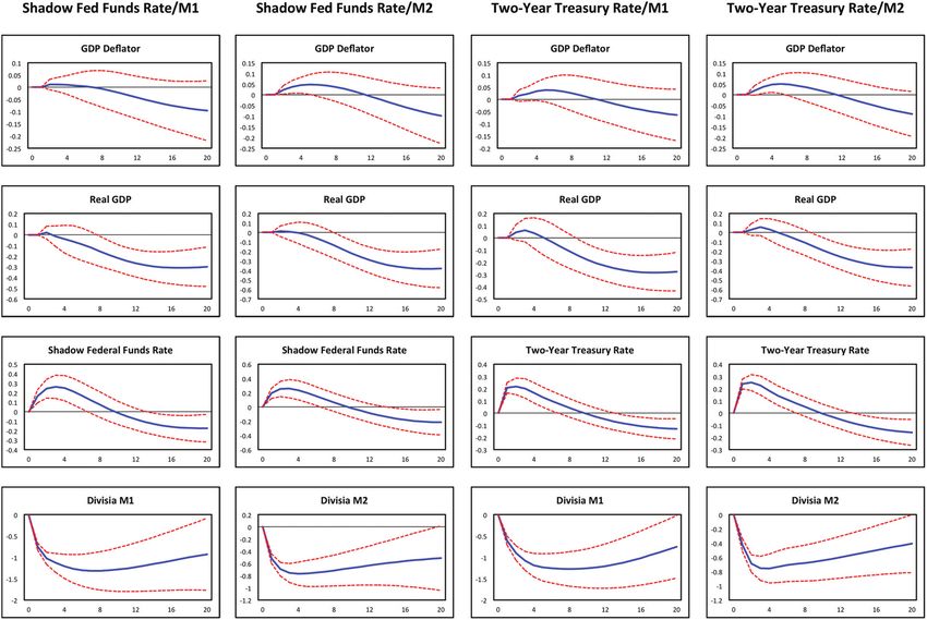
shock (solid line) together with plus-and-minus one standard error bands (dashed lines).Figure 4. Monetary Policy Shocks: Historical and Counterfactual
Vol. 14 No. 2
Targeting Constant Money Growth
183
Note: Panels show the historical path for the identified monetary policy shock and counterfactual paths required to support
constant rates of money growth.184 International Journal of Central Banking March 2018
persistently later on.11 The initial upward movement in the price
level gets magnified when the two-year Treasury yield is used to
measure the interest rate, suggesting that the shadow federal funds
rate is more useful in identifying monetary policy shocks over the
entire 2000–16 sample period.12 The initial increase in prices also
becomes larger when Divisia M2 replaces Divisia M1 as the mea-
sure of money. Across all four data sets, however, the effects of the
monetary policy shock on the aggregate price level are small and
imprecisely estimated. The absence of strong effects of monetary pol-
icy on inflation is, in fact, a feature that runs consistently through
all of the results that follow.
Table 5 reports the fraction of the forecast error variances in real
GDP and the GDP deflator attributable to monetary policy shocks,
again identified with the non-recursive specification in (9). Although
their standard errors, computed in the same way as for the impulse
responses described above, are large, these variance decompositions
attribute to monetary policy shocks about 20 percent of the forecast
errors in real GDP over horizons of four to five years. By contrast,
monetary shocks explain relatively little of the volatility in the GDP
deflator.
As shown previously in figure 1, Divisia M1 and M2 grew at
average annual rates of 9 and 6.75 percent, respectively, between
2008:Q1 and 2016:Q2. With stable velocity, of course, those rates
of money growth would have translated into similarly robust rates
of growth in nominal spending and resulted in much faster rates of
real GDP growth and inflation than those seen historically. The sub-
stantial declines in velocity shown in the same figure, however, imply
that even more rapid monetary expansion was needed to fully stabi-
lize the economy. In addition, because money growth itself exhibited
wide fluctuations about its mean, falling sharply in particular when
the Fed briefly suspended its quantitative easing in 2010, monetary
11
As shown in a previous draft of this paper, available as Belongia and Ireland
(2016c), the price puzzle appears in the impulse response to an identified mone-
tary policy shock even when an index of commodity prices is included in the list
of series used to estimate the non-recursive model.
12
This observation also is consistent with Swanson and Williams (2014), which
shows that while the two-year Treasury yield reacted fully to Federal Reserve pol-
icy actions through 2010, the zero lower bound began constraining its movements
in 2011.Table 5. Forecast Error Variance Decompositions from
Non-recursive Vector Autoregression
Shadow Federal Funds Rate/M1 Shadow Federal Funds Rate/M2
Quarters
Ahead GDP Deflator Real GDP GDP Deflator Real GDP
2 0.23 0.12 1.05 0.05
(0.88) (0.70) (1.78) (0.44)
Vol. 14 No. 2
4 0.21 0.18 2.62 0.02
(1.15) (0.90) (4.07) (0.16)
8 0.08 2.11 2.20 1.56
(0.32) (5.34) (4.61) (4.20)
12 0.43 9.02 1.45 10.17
(1.90) (11.43) (3.37) (12.66)
16 1.63 17.83 1.83 21.39
(5.24) (15.54) (2.72) (16.17)
20 3.48 23.40 3.98 26.96
(9.73) (17.04) (8.91) (15.99)
Two-Year Treasury Rate/M1 Two-Year Treasury Rate/M2
Quarters
Ahead GDP Deflator Real GDP GDP Deflator Real GDP
2 0.47 0.56 0.75 0.27
(1.43) (1.57) (1.71) (1.08)
4 1.37 0.60 3.04 0.47
(3.18) (2.09) (4.51) (1.87)
8 1.25 1.02 2.46 1.09
Targeting Constant Money Growth
(3.74) (1.76) (4.86) (2.31)
12 0.79 5.99 1.59 7.37
(2.43) (8.28) (3.52) (9.93)
16 1.02 13.90 1.91 16.46
(1.73) (13.70) (2.65) (14.11)
20 1.94 19.68 3.91 22.02
(4.95) (15.37) (7.55) (15.00)
185
Note: Each entry shows the percentage of the forecast error variance in the GDP deflator or real GDP due to the identified monetary policy
shock at the indicated horizon. Standard errors are in parentheses.186 International Journal of Central Banking March 2018
policy may have contributed to some of the slow growth and inflation
experienced during the period of recovery from the Great Reces-
sion. Evidence on this conjecture can be seen in the top row of
figure 4, which plots the historical series for monetary policy shocks
implied by the estimated, non-recursive SVAR. Strikingly, most of
the policy disturbances realized during 2009 and 2010 are positive:
since shocks with this sign are associated with higher interest rates
and slower rates of money growth, they signal that monetary pol-
icy was unexpectedly tight throughout this period. Along with the
impulse responses in figure 3 and variance decompositions in table
5, therefore, the historical shocks in figure 4 show that, accord-
ing to the estimated model, it was not until 2011 and 2012 that
Federal Reserve policy began to lend full support to the economic
recovery.
These observations suggest that the lesson drawn from U.S. mon-
etary history by Friedman and Schwartz (1963) and Brunner and
Meltzer (1968) continues to have relevance today. By interpreting
low nominal interest rates as a sign of monetary ease and neglecting
signs of tightness implied by a comparison of trends in money sup-
ply and money demand, it is possible to understand how the Federal
Reserve contributed to the length and severity of the Great Depres-
sion and why the Fed behaved as it did during the Great Recession.
But, again, these observations beg the following questions: Would
switching to Milton Friedman’s (1960) k-percent rule for constant
money growth once the zero lower bound for the funds rate had been
reached—an option specifically mentioned by Taylor (2009)—have
been feasible? If so, would policy conducted according to that con-
stant money growth rule have led to a more rapid, or at least a more
stable, recovery and expansion following the recession? And would
targeting faster rates of money growth have generated even more
favorable outcomes?
To answer these questions, figures 4–7 illustrate in detail and
table 6 summarizes the results from three counterfactual experi-
ments, in which the estimated non-recursive SVAR is used to simu-
late the effects of constant money growth rate policies. The remain-
ing panels of figure 4 show the hypothetical series of monetary policy
shocks from 2008:Q1 forward that, when fed through the estimated
model, keep Divisia M1 or M2 growing along a constant path even
as all other shocks take on their historical values. The first set ofFigure 5. Counterfactual Simulations: Constant 9 Percent M1 Growth
or 6.75 Percent M2 Growth Vol. 14 No. 2
Targeting Constant Money Growth
187
Note: Each panel shows the historical path (dashed line) for the indicated variable, together with the counterfactual path
(solid line) of the same variable surrounded by plus-and-minus one standard error bands (dotted lines).You can also read