Team Payroll Versus Performance in Professional Sports: Is Increased Spending Associated with Greater Success?

Team Payroll Versus Performance in Professional Sports:
 Is Increased Spending Associated with Greater Success?

 Grant Shorin

 Professor Peter S. Arcidiacono, Faculty Advisor
 Professor Kent P. Kimbrough, Seminar Advisor

 Duke University
 Durham, North Carolina
 2017

Grant graduated with High Distinction in Economics and a minor in Statistical Science in May 2017. Following
graduation, he will be working in San Francisco as an Analyst at Altman Vilandrie & Company, a strategy
consulting group that focuses on the telecom, media, and technology sectors. He can be contacted at
grant.shorin@gmail.com.

Acknowledgements

 I would like to thank my thesis advisor, Peter Arcidiacono, for his valuable guidance. I
would also like to acknowledge my honors seminar instructor, Kent Kimbrough, for his
continued support and feedback. Lastly, I would like to recognize my honors seminar classmates
for their helpful comments throughout the year.

 2

Abstract

 Professional sports are a billion-dollar industry, with player salaries accounting for the
largest expenditure. Comparing results between the four major North American leagues (MLB,
NBA, NHL, and NFL) and examining data from 1995 through 2015, this paper seeks to answer
the following question: do teams that have higher payrolls achieve greater success, as measured
by their regular season, postseason, and financial performance? Multiple data visualizations
highlight unique relationships across the three dimensions and between each sport, while
subsequent empirical analysis supports these findings. After standardizing payroll values and
using a fixed effects model to control for team-specific factors, this paper finds that higher
payroll spending is associated with an increase in regular season winning percentage in all sports
(but is less meaningful in the NFL), a substantial rise in the likelihood of winning the
championship in the NBA and NHL, and a lower operating income in all sports.

JEL Classification: Z2; Z20; Z23; J3.

Keywords: Sports; Payroll; Performance; Competitive Balance.

 3

TABLE OF CONTENTS PAGE

1. Introduction .................................................................................................................................5

2. Literature Review........................................................................................................................7

3. Theoretical Framework and Empirical Regulators ...................................................................11
 3.1. Labor Market in Professional Sports ..........................................................................12
 3.2. Competitive Balance ...................................................................................................13
 3.2.i. Within-Season Variation................................................................................14
 3.2.ii. Between-Season Variation............................................................................15
 3.2.iii. Lorenz Curve ...............................................................................................17
 3.3. Salary Caps .................................................................................................................20
 3.4. Free Agency ................................................................................................................21

4. Data ...........................................................................................................................................22
 4.1. Discussion of Data Sources ........................................................................................22
 4.2. Preliminary Baseline Analysis ....................................................................................23
 4.3. Data Transformations..................................................................................................30

5. Empirical Analysis and Discussion ..........................................................................................31
 5.1. Regular Season Success ..............................................................................................33
 5.2. Postseason Success .....................................................................................................39
 5.3. Financial Success ........................................................................................................43
 5.4. Statistical Comparison Between Leagues ...................................................................48

6. Conclusion ................................................................................................................................50

7. References .................................................................................................................................54

8. Data Sources .............................................................................................................................55

9. Appendix ...................................................................................................................................56

 4

1 Introduction
 During their respective 2015 seasons1, the four major North American professional sports
 leagues – comprised of the Major League Baseball (MLB), National Basketball Association
 (NBA), National Hockey League (NHL), and National Football League (NFL) – cumulatively
 earned $30.52 billion in revenue and spent $25.53 billion in total expenditures. Player expenses
 accounted for the largest component at $14.97 billion, responsible for nearly 60% of total
 expenditures. Table 1 provides a one-year snapshot into each league’s financial data, but this
 proportion has remained relatively constant over the past 20 years, primarily due to
 arrangements in each sport’s collective bargaining agreement between each league and their
 respective players’ association. The significant portion spent on player personnel illustrates their
 perceived key role in driving organizational performance (both on and off the field). However,
 the exact relationship between team payroll and performance is unclear, leading one to consider
 if paying players more money is linked to greater achievement. One would believe that a
 player’s salary should be based on their athletic prowess, with compensation commensurate
 with capability, but the full impact of this relationship remains unclear. Specifically, the
 examination between a team’s payroll and their resulting performance merits further
 quantitative and qualitative analysis in order to understand if increased spending on players is
 associated with greater success, as measured in a multitude of ways.
Table 1 – League Financials for 2015 Season ($ Billions)
 Total Total Player Players Expenses Operating
 Revenue Expenses Expenses as % of Total Income
 MLB $8.39 $7.72 $4.42 57.25% $0.68
 NBA $5.87 $4.92 $2.73 55.47% $0.95
 NHL $4.10 $3.66 $2.07 56.52% $0.44
 NFL $12.16 $9.23 $5.75 62.29% $2.92
 Total $30.52 $25.53 $14.97 58.64% $4.99
Note. Financial figures obtained from Forbes’ annual estimates.
 The four major sports leagues all employ different policies regarding player
compensation, but the key difference deals with the restrictiveness of their salary caps, which
create limits on how much teams can spend on player salaries. Understanding these differences is

1
 “2015 season” refers to the season that began in 2015 (some of the leagues have seasons that start in one year and
finish in the next). See Appendix Table A1 for additional key differences across sports.

 5

a fundamental element of this research on player compensation and team performance. When
ranking each league based on the amount of freedom teams have to decide how much they want
to spend, the MLB allows the greatest flexibility and is closely followed by the NBA, while the
NHL and NFL have the strictest limits (Staudohar, 1998). Throughout the entirety of the paper, I
will refer to each sport in the same sequence (MLB, NBA, NHL, and NFL), which has been
ordered from least to most restrictive. The MLB has no salary cap and instead implements a
luxury tax, whereby teams whose total payroll exceeds a certain figure (determined annually) are
taxed on the excess amount in order to discourage teams from having a substantially higher
payroll than the rest of the league. Since 2003, only seven different franchises have had to pay
luxury taxes, with typically two to three teams paying fees each year (ESPN, 2015). The NBA
uses a combination of a soft cap and a luxury tax, permitting several significant exemptions that
allow teams to exceed the pre-defined limit, but also requiring a luxury tax payment if the team
payroll exceeds the cap by a certain amount. Unlike the MLB, this limit is frequently surpassed,
as 26 franchises have had to pay luxury taxes since 2003, with roughly five to six offenders each
year (Shamsports, 2015). Lastly, the NHL and NFL employ hard caps, firmly restricting the total
amount a team can spend, allowing essentially zero flexibility2 (in fact, teams have been severely
punished when they were found to have paid players in excess of the cap). While it is evident
that the four major U.S. sports leagues utilize a continuum of salary caps, its impact on the
relationship between salary spent and team success has remained unclear.
 This research aims to empirically analyze the relationship between a team’s payroll and
the success they achieve, comparing the findings across the four major North American
professional sports leagues. While there are many ways to gauge success, this research examines
the relationship between a team’s payroll and performance across three dimensions: regular
season success, postseason success, and financial success. These metrics diverge between
leagues, as their respective regular seasons have different characteristics, playoffs have unique
structures, and team finances greatly differ across leagues, which all complicate a perfect apples
to apples comparison. However, the overarching idea of examining the statistical significance of
any potential correlations remains consistent throughout. More generally, although these metrics

2
 The NFL salary cap allows teams to “carryover” unused cap space from the previous year. For illustrative
purposes, assume that the salary cap in the NFL for the 2014 and 2015 seasons was $140 million. If the San
Francisco 49ers spent $130 million in 2014, $10 million would rollover into the next season, allowing them to spend
up to $150 million in 2015.

 6

are not independent from one another, they represent three of the most crucial benchmarks of
success through their measurement of regular season achievement, postseason accomplishment,
and financial performance, and are relevant to each of the leagues.
 This research begins by highlighting the key findings of prior relevant literature. Next, it
explains the theoretical framework behind some central concepts including the labor market in
professional sports, competitive balance, salary caps, and free agency. Subsequently, the paper
quantitatively analyzes payroll data between from 1995 through 2015 (selected based on data
availability and the desire to examine as far back as possible) across the four leagues, revealing
how team spending is related to various metrics of success. Idiosyncratic differences across the
leagues are investigated further to provide rationale that may explain the results. This component
is tightly connected to the quantitative analysis and various additional statistical comparisons,
but also strives to incorporate qualitative explanations that are based on the fundamental nature
of each sport. Ultimately, the paper aims to determine the relationship between payroll and
success and examine the underlying factors driving results both within and across leagues.

2 Literature Review
 Many have previously researched the intersection between sports and finance. Within the
area, a variety of subtopics have been explored. Most relevant to this paper, some have
previously sought to examine if team payroll is linked with team performance. However, while
there does exist significant work on this relationship, most of the prior literature has
predominantly focused on baseball. While this correlation has been explored in isolation, a
comparison across the four major leagues remains uncharted. Therefore, great gains can be made
in undertaking this research and comparing the results from the quantitative and qualitative
analysis.
 In a paper that most closely mirrors the intended analysis of this research, Hasan (2008)
examined data from the MLB from 1992 to 2007 and investigated the relationship between team
performance and payroll, comparing the winning percentages and payrolls of MLB teams. Hasan
looked at a team’s performance over the course of the 162-game regular season, believing that
the larger sample size of games would provide a more accurate picture of a team’s success
(versus extending into the playoffs). Additionally, Hasan decided against using a team’s regular
season ranking as an indicator of success, illustrating the inherent problem associated with such

 7

an approach by explaining that difference between a team ranked 5th and a team ranked 15th is
not necessarily by a factor of three (i.e. the 5th ranked team did not win three times as many
games as the 15th). Ultimately, Hasan ran the following OLS regression model:
 WinPercentt = a + b*Payscalet + et (1)
where Payscalet is a team’s actual payroll divided by the average payroll for the overall league in
year t. He found there was a statistically significant positive association between payroll and
regular season winning percentage. Specifically, Hasan stated that “sufficient evidence was
found that regular season outcomes are highly influenced by how much the teams spend on their
players” (p. 4). Some of Hasan’s methodology forms the baseline of this paper, but this research
attempts to greatly expand upon his approach. While his rationale behind solely examining the
regular season is correct (larger sample size of games may be more indicative of a team’s
ability), testing whether regular season performance extends into the postseason provides many
additional rich insights. Teams are frequently judged by how they fare in the playoffs, so solely
examining the regular season ignores a critical component of success. Additionally, Hasan’s
scope narrowed in on MLB, whereas this paper explores that relationship across multiple
leagues. Nevertheless, this paper expands on Hasan’s work by leveraging (and extending) certain
statistical methodologies as well as validating the relationship between performance and payroll
across the major sports leagues.
 In 2000, the MLB commissioned a study to examine if revenue disparities among clubs
were damaging competitive balance and sought recommendations on structural reforms to
address the problem. For analytical purposes, Levin, Mitchell, Volcker, and Will (2000) divided
the clubs into quartiles by ranking them (based on payroll) from high to low and separating the
clubs into four roughly equal buckets (i.e. Quartile I consisted of the top 25% highest spending
teams and Quartile IV included the bottom 25% lowest spending teams). Among the many
findings, Levin et al. found that a large and growing revenue disparity existed, which created
problems of chronic competitive imbalance, a trend that substantially worsened following the
strike shortened 1994 season. Additionally, Levin et al. wrote that “although a high payroll is not
always sufficient to produce a club capable of reaching postseason play—there are instances of
competitive failures by high payroll clubs—a high payroll has become an increasingly necessary
ingredient of on-field success” (p. 4). From this perspective, Levin et al. explain that a high
payroll does not necessarily ensure high performance, but rather is a prerequisite to achieve

 8

success, severely impacting the league’s competitive balance. Furthermore, Levin et al.
delineated a methodology for determining payroll parity. They explained that they believe an
indicator of parity would be a ratio of approximately 2:1 between the average payroll of Quartile
I clubs to that of Quartile IV clubs. However, during the three years preceding the release of their
study, they found that the ratio of the average payroll of Quartile I teams divided by Quartile IV
was 1.5:1 in the NFL, 1.75:1 in the NBA, and over 2.5:1 in the MLB, reaffirming their stance
that the MLB lagged behind the other two in terms of payroll competitive balance. Overall,
Levin et al.’s study clearly elucidates that a team’s payroll is associated with their postseason
success in the MLB, and offers an operational approach to quantifying and comparing payroll
parity across leagues3.
 While less prevalent, some studies have researched the relationship between player
salaries and team financial performance. In a 2015 paper, “Performance or Profit: A Dilemma for
Major League Baseball,” Steven Dennis and Susan Nelson examined the effect of team payrolls
on the revenues, profits, and winning percentages of MLB teams from 2002 to 2010. They ran
regressions on a variety of financial metrics, but the two most relevant include:
 TeamRevenuei,t = a + b*TeamSalaryi,t + et (2)
 TeamOperatingIncomei,t = a + b*TeamSalaryi,t + et (3)
which both yielded some interesting conclusions. Namely, Dennis and Nelson write that “the
motivation of a MLB team owner may not be simply to maximize profits; maximizing winning
percentages also comes into play. Although team revenues are higher when player salaries are
higher, the increase in revenue is less than one-for-one with an increase in player salaries. As a
result, gross profit margin decreases with player salary increases” (p. 6). From this perspective,
we see that organizations may be faced with a competing choice of whether to maximize profits
or winning. When franchises spent more money, Dennis and Nelson found that teams tended to
have higher winning percentages. However, although revenues also generally increased as teams
had higher payrolls, the associated expenses outpaced this rise in revenue, causing gross profit
margin (computed as revenue less payroll, divided by revenue) to fall. In subsequent analysis,
this paper computes analogous regressions and examines a similar contrast between winning and

3
 Updated calculations for all four leagues have been reported in Figure 8 and are discussed in Section IV of this
paper.

 9

profits, comparing results across leagues and providing explanations based on infrastructural
differences.
 In yet another study on the MLB, Hall, Szymanski, and Zimbalist (2002) utilized team
payroll data between 1980 and 2000 to examine the connection, implementing Granger causality
tests to establish whether the relationship runs from payroll to performance or vice versa. Hall et
al. write that although “there is no evidence that causality runs from payroll to performance over
the entire sample period, the data shows that the cross-section correlation between payroll and
performance increased significantly in the 1990s” (p. 149). This finding illustrates an important
idea that is considered throughout the entirety of this paper. The relationship between payroll and
performance is not static, meaning that the results may vary over time. Although this may appear
at first glance to be an unsettling conclusion, it reaffirms the importance of understanding
important events and trends that have occurred in the four leagues over the course of the past 20
years. The key takeaway is that while statistical methods may uncover certain patterns, a deep
historical knowledge of the idiosyncratic elements of each sport are essential to uncovering the
underlying influence.
 Differences in correlations between payroll and success across the leagues may
potentially be derived from the underlying nature of each sport. In an article comparing the labor
markets in the MLB and NFL, Dubner (2007) attempts to explain the diverging power dynamics
in each league. At a high level, a commonly held belief is that players have more influence in
MLB, while a team’s ownership has more power in the NFL (often at the expense of individual
players). This manifests itself in higher paying contracts with more guaranteed money for
baseball players. Diving deeper into the economics of each sport, the MLB and NFL operate
under dissimilar business models. MLB teams are run at a much more local level, with less than
25% of all league revenues distributed evenly among all 30 organizations. The remaining 75% of
revenues are earned and kept at a local level, with a disproportionate share going to franchises in
large markets with strong team brands and greater on-field success. This increases the volatility
for the primary revenues of a baseball team (ticket sales, luxury suite rentals, local broadcast
ratings, and subsequent rights fees) which can all rise and fall with winning and losing seasons.
Conversely, 80% of the NFL’s revenue is divided evenly among the 32 teams, and empirical
evidence clearly shows that market size has little impact on the revenue base of an NFL club.
Although revenue sharing and market factors are tangential to the core focus of this paper, they

 10

provide profound intuitions into the structural differences of the labor markets of the two sports,
possibly explaining potential dissimilarities that may emerge.
 Given the magnitude of team payrolls, many have attempted to analyze whether higher
player payrolls are associated with increased team success. While many previous studies have
thoroughly explored this area, so far much of the research has concentrated on individual salaries
and the player’s corresponding performance. Of the research that has been completed at the team
level, most has focused primarily on baseball. However, limited research has been made in
comparing the relationship between the four major professional sports leagues. While the
existing research has predominantly used a couple methodologies (pay-scales and pay-quartiles),
this paper intends to build upon each of them to best match the metric of success being examined
(regular season, postseason, and financial success).
 This paper contributes to the existing research in a variety of ways, delivering rich
insights into the differences across the various leagues and juxtaposing the relationships across
several benchmarks of success. At its core, this paper supplements the current research in five
ways. First, all four professional sports leagues have been included in the analysis (rather than
only one), allowing for relative comparisons across leagues. Second, the relationship has been
examined across multiple metrics of success, instead of solely looking at regular season winning
percentage. Third, the empirical methodology is more robust, controlling for team-specific
factors. Fourth, this work provides an updated time frame of analysis, examining seasons from
1995 through 2015. Lastly, this paper attempts to highlight league and team-specific factors in
order to logically explain divergent findings.

3 Theoretical Framework and Empirical Regulators
 The massive amount of money involved in professional sports underscores how
organizations are increasingly run like traditional businesses, influencing how team executives
make decisions on a day-to-day basis. Since every organization has a unique utility function,
each places a different priority on team success and financial profit. Accordingly, executives
make personnel decisions under a diverse set of preferences, creating a labor market where teams
must decide how to best leverage their various assets to achieve their desired goals. There are a
handful of critical concepts that will provide essential context for understanding various dynamic

 11

factors that underpin the relationship between payroll and performance. The following
subsections will outline these concepts and relate them to the core research objectives.

3.1. Labor Market in Professional Sports
 The primary method used by franchises to improve team performance is to acquire and
retain top talent (via trade, free agency, draft, or re-signing), frequently competing with other
organizations to employ the best players. This competitive dynamic means teams strive to
provide the most attractive offer, which can include an array of factors beyond money, such as
elite coaching, high-class medical services, and premier training facilities. To understand the
basic economics of the labor market, it is helpful to briefly evaluate the situation from the
demand (team) and supply (player) perspective.
 On the demand side, franchises value players based on the benefits that they will
provide. While this most importantly centers upon their ability to perform on the field, it also
includes a myriad of ancillary factors such as a player’s leadership ability, personality fit with
existing teammates, and marketing potential. Based on a team’s complete evaluation of a player,
they can decide if they would like to attempt to employ that individual by offering compensation
that is representative of how much they value that athlete. If the labor market was perfectly
efficient, each player would go to the team that values them the most, with all teams offering
contracts that matched how much they valued that specific individual. However, that is not
necessarily the case in practice. An assortment of factors distort the market, including salary caps
which introduce a constraint on the amount a team can pay players, minimum salaries that
establish a price floor, and maximum salaries that set a price ceiling. At the end of the day,
personnel decisions are made by humans who may be motivated by different goals, whether that
be winning, generating profits, or simply retaining their job. While these all can inject potential
distortions between what an athlete is theoretically worth and what they actually earn, players
generally receive compensation that is proportionate with their abilities. Therefore, one would
expect that teams that spend the most amount of money will be able to accrue the greatest
amount of talent, presumably leading to the greatest success.

 12

Figure 1. Competing preferences in professional labor market.
 Since contracts must be mutually agreeable, it is important to view things from players’
perspectives as well. The contrasting preferences of teams and players are illustrated in Figure 1,
whereby the “contract zone” represents the negotiation range in which both sides might agree on
the terms of a contract (Leeds and Allmen, 2011). The primary (and most quantifiable) factor at
an organization’s disposal is the financial compensation they are willing to offer in exchange for
a player’s services, and at the end of the day, like any other job, professional athletes tend to
accept offers where they receive the highest compensation. Therefore, this paper is
predominantly framed from the perspective of teams since they have the power to determine the
strategic priorities of their organization.

3.2. Competitive Balance
 One of the oldest adages in sports is that on any given day, each team has a chance to
beat the other. If only a few teams regularly won and the rest almost always lost, games would be
decidedly less interesting. Since professional sports fundamentally serve as a form of
entertainment, successful leagues must be based on relatively even competition. The concept of
competitive balance is central to my topic, since one of the primary mechanisms leagues use to
increase parity is the creation of payroll restrictions (like salary caps and luxury taxes).
 While there are many opinions on the matter, there are two prevalent approaches to
measuring competitive balance (Leeds and Allmen, 2011). The first method focuses on team
performance over the course of a single season. By examining the dispersion of winning
percentages, one can see the disparity between high and low performing teams. The second
approach looks across multiple seasons, measuring the concentration of championships over a
given period. Both approaches have merit, so it is important to consider both types of variation in
order to get a more complete picture.

 13

3.2.i. Within-Season Variation
 The first approach to quantifying competitive balance looks at the dispersion of teams in
a given season. The subsequent procedures for computing competitive balance closely follow
those delineated by Brad Humphreys in his widely-cited paper, “Alternative Measures of
Competitive Balance in Sports Leagues” (2002). Generally, measures of within-season variation
are based on the standard deviation of winning percentages. In professional sports, there is a
winner and loser in each game, so the average winning percentage is 0.500, where the standard
deviation is defined:
 4 (()*+ ./.1//)3
 ,,-
 ",$ = ,56
 (4)
 7

where 

where 0.50 indicates each team has a 50% chance of winning and G is the number of games in a
season. These calculations reveal an “ideal” standard deviation of 0.039 in the MLB, 0.055 in the
NBA and NHL, and 0.125 in the NFL. Using these two measures of average variation, we can
define the Competitive Balance Ratio (CBR) as follows:
 AB
 = (6)
 AC

4
 To illustrate, imagine flipping a fair coin four times. Applying the binomial distribution, we know that the
probability of observing an extreme outcome of all heads or all tails is 12.5% (1 out of 8 times). If a coin is flipped
10 times, the odds of getting all heads or all tails plummets to 0.2% (1 out of 512 times). As we continue to increase
the number of coin flips, the chances of an extreme outcome become increasingly remote.

 14

Table 2 reveals that the NBA has the highest ratio between actual standard deviation and the
theoretical value at 2.83, indicating that basketball has the least parity in-season. On the other
end of the spectrum, the NFL has the lowest CBR at 1.52, suggesting the greatest parity amongst
all leagues. The MLB and NHL sit between the other two sports, with ratios of 1.77 and 1.62,
respectively. From this initial examination, we can begin to see that there exists fundamental
differences across the four leagues. When comparing competitive balance from a within-season
perspective, we see that the NBA had the least parity while the NFL had the greatest equity, with
the MLB and NHL finishing in between the other two. Loosely, this follows what one would
expect given each leagues’ salary cap restrictiveness, as the two sports with strongest caps
(hockey and football) showed the greatest competitive balance.
 Table 2 – Dispersion of Winning Percentages (1995 – 2015)
 MLB NBA NHL NFL
 Mean SD 0.070 0.156 0.090 0.190
 Ideal SD 0.039 0.055 0.055 0.125
 CBR 1.77 2.83 1.62 1.52

3.2.ii. Between-Season Variation
 The second approach to measuring competitive balance attempts to look at how teams
finish differently on a year-to-year basis. Graphically, one way to examine this is by comparing
how well a team does from one year to the next5. In Figure 2, I have overlaid standard boxplots
on top of violin plots6 to show how much a team’s winning percent tends to change from one
season to the next. Ranking them from most to least persistent, we see that teams in the MLB and
NHL generally had fairly similar winning percentages each year. Teams in the NBA tended to
have a little more turnover, while the NFL clearly showed the greatest year-over-year changes in
how well a team performed. However, it is important to note that this does not control for
differences in the number of games in a season, which we previously mathematically showed
that extreme outcomes are more likely when there are fewer games. Nevertheless, Figure 2
provides an informative baseline for subsequent analysis.

5
 The values are calculated by subtracting the previous years’ win percentage from the current one. For instance, if a
team won 40% of games this year and 60% last year, that would correspond to a change of -20%.
6
 Boxplots demarcate basic distribution values including the median, 25th percentile, and 75th percentile. Violin plots
are mirrored histograms, with the width of the plot corresponding to the frequency of that event. That means that
wider areas correspond to more common outcomes.

 15

50%
Change in Win Percent

 25%

 0%

 −25%

 −50%

 MLB NBA NHL NFL

Figure 2. Change in team win percent between consecutive years from 1995 to 2015.
 Computationally, there are multiple ways of investigating how much league results
change year-over-year. One common approach is to apply the Herfindahl-Hirschman Index
(HHI), which was developed to measure the concentration of firms in an industry but can be used
to measure the concentration of league championships. It is defined:
 F, G
 = < (7)
 +

where < is the number of championships team i won in a given period and T is the number of
years in the period. The minimum of HHI is 1/N, which corresponds to a scenario in which all
teams alternate championships, while the maximum is 1, which would indicate complete
imbalance (with one team winning every time). In Table 3, I have calculated the results from
1995 through 2015. When considering the concentration of championships, the NBA has the
largest HHI value at 0.17, indicating that it had the highest concentration of winning. This makes
intuitive sense, since four teams (the Los Angeles Lakers, San Antonio Spurs, Chicago Bulls,
and Miami Heat) accounted for 16 of the 21 titles won during that span. The NFL had the
smallest HHI value of 0.11, further reinforcing its status as the league with the greatest parity.
This figure is somewhat buoyed by the New England Patriots’ four titles and the Denver
Broncos’ three championships, but is consistent with history as 12 different franchises have won
during the past 21 seasons. Again, the MLB and NHL reside in between the NBA and NFL, as

 16

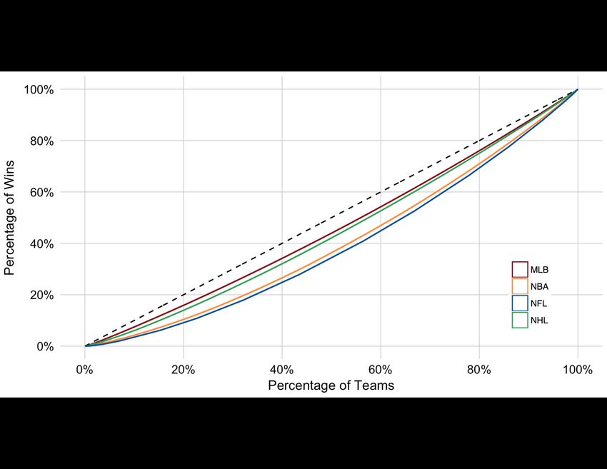
each league only has a few franchises that have won three or more titles, with the majority of the
other championships awarded to single-title teams. When comparing competitive balance from a
between-season perspective, we see a familiar pattern, with the NBA having the least parity and
the NFL showing the greatest balance, with the MLB and NHL in between.
 Table 3 – Distribution of Championships (1995 – 2015)
 MLB NBA NHL NFL
 Titles by Yankees––5 Lakers––5 Red Wings––4 Patriots––4
 Franchise Giants––3 Spurs––5 Blackhawks––3 Broncos––3
 Red Sox––3 Bulls––3 Avalanche––2 Giants––2
 Cardinals––2 Heat––3 Devils––2 Packers––2
 Marlins––2 Cavaliers––1 Kings––2 Ravens––2
 Angels––1 Celtics––1 Penguins––2 Steelers––2
 Braves––1 Mavericks––1 Bruins––1 Buccaneers––1
 Diamondbacks––1 Pistons––1 Ducks––1 Colts––1
 Phillies––1 Warriors––1 Hurricanes––1 Cowboys––1
 Royals––1 Lightning––1 Rams––1
 White Sox––1 Stars––1 Saints––1
 Seahawks––1
 HHI 0.13 0.17 0.12 0.11

3.2.iii. Lorenz Curve
 Lorenz curves can be used to graphically express competitive balance. Commonly used
in economics, Lorenz curves illustrate how evenly a resource is distributed throughout a
population. Applied to sports, we can use the same logic to see how equitable wins are in each
league. To understand how it is interpreted, consider the NBA’s 2015 regular season. Since all
30 teams play an 82-game schedule, there are 1,230 total games (and hence 1,230 possible wins)
over the course of the season. The three worst teams (the Philadelphia 76ers, Los Angeles
Lakers, and Brooklyn Nets) combined to win only 48 games. Thus, the bottom 10 percent of
NBA teams combined to account for only 3.9% of the NBA’s wins. Conversely, the three best
teams (the Golden State Warriors, San Antonio Spurs, and Cleveland Cavaliers) collectively won
197 games, meaning that the top 10 percent of teams accounted for 16.0% of the NBA’s wins.
Undertaking a similar analysis for the MLB’s 2015 season reveals a more equitable picture.
During a 162-game season, the thirty teams play a total of 2,430 games7. The three weakest

7
 A game between the Detroit Tigers and the Cleveland Indians was canceled, so there were only 2,429 games
during the 2015 season.

 17

teams (the Philadelphia Phillies, Cincinnati Reds, and Atlanta Braves) combined to win 194
games, accounting for 8.0% of the MLB’s wins. Meanwhile, the three strongest teams (the Saint
Louis Cardinals, Pittsburgh Pirates, and Chicago Cubs) accumulated 295 wins, accounting for
12.1% of the MLB’s wins. Hence, we see that the 2015 MLB season experienced a more
equitable distribution of wins amongst its teams.
 In a perfectly equal world, every team would win an equal amount, meaning that any 10
percent of the population will account for 10 percent of the wins. While this would not make for
a very entertaining league, this “ideal” Lorenz curve represented by the diagonal dashed line in
Figure 3. As imbalance increases, the actual Lorenz curve sags further below the ideal. Figure 3
depicts that the MLB and NHL closely resemble one another and show the greatest parity, while
the NBA and NFL show greater inequity. This conclusion slightly diverges from previous
findings that showed the NFL had the greatest parity. However, this is consistent in justifying the
calculations used to find each league’s CBR, where we found that increasing the number of
games decreases the dispersion of winning percentages. More interestingly, Figure 3 seems to
show a curious dichotomy between sports, as the Lorenz curves for the MLB and NHL closely
resemble one another, as do the curves for the NBA and NFL. One noteworthy characteristic is
that runs in baseball and goals in hockey tend to be harder to come by, with most games
generally finishing in single digits. Conversely, games in the NBA and NFL tend to have much
higher scores. Thus, in sports where games are decided by fewer units, luck appears to play a
more significant role, as a few particular plays can have a profound impact on the final score
(and the outcome of the game). This underscores an important note that the fundamental nature
of each sport differs, and that perfect comparisons across leagues are likely unreasonable.

 18

Figure 3. Lorenz Curve for regular season win totals from 1995 through 2015.
 In summary, there are numerous ways to measure parity, but no single method is
unilaterally superior. Rather, to fully examine the competitive landscape, it is important to
consider both within-season balance and between-season balance. Across the various methods,
the NBA showed the least parity, while the NFL tended to have the greatest balance, with the
MLB and NHL generally residing in between. Across all sports, leagues are concerned about all
these forms of competitive balance, since fan interest is impacted by it, which corresponds to
attendance, television ratings, and league profits. Although by no means the sole explanation, it
may be no coincidence that the league with the greatest parity (the NFL) is by far the most
profitable, recording an operating income that was approximately $850 million higher than the
three other leagues combined8. Succinctly stated, competitive balance is crucial to a league’s
ultimate success. Leagues have astutely recognized the importance of ensuring parity and have
worked to implement various tools to provide a level playing field.

8
 Refer to Table 1 for additional league finance statistics. During the 2015 season, the NFL earned $2.92 billion in
operating income, while the other three combined to account for $2.07 billion.

 19

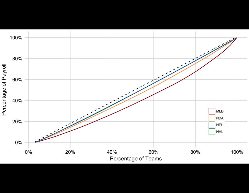
3.3. Salary Caps
 One of the primary ways leagues try to increase parity is by implementing salary caps
and other related payroll restrictions such as luxury taxes9. Leagues strive to maintain
competitive balance, hoping for fewer contests where the winner can easily be predicted in
advance. By limiting the amount of money a team can spend on players, leagues aim to reduce
the difference in talent levels between low-spending and high-spending teams, with the objective
of establishing a more equal playing field10. Since teams are located in different sized markets,
ranging from desolate Green Bay (population 100,000) to dense New York City (population 8.4
million), there exists an inherent inequity between the amount of money a team can earn from its
local market, which thereby affects how much money they have available to spend on players.
Consequently, based in part on the premise that money can buy success, all leagues have
implemented measures to reduce these core differences in available resources, whether that be a
salary cap (NBA, NHL, and NFL) or a luxury tax (MLB and NBA). Salary caps set upper and
lower limits to payrolls and are based on a percentage of qualifying league revenues (with
definitions varying slightly by league), where owners are obligated to spend a defined share of
the qualifying revenues. The NHL and NFL have a hard cap, which sets a firm limit and permits
no exemptions. Meanwhile, the NBA utilizes a soft cap, which specifies a salary ceiling but
allows many exceptions. There are dozens of exemptions, but the three most widely known are
the Larry Bird Exception11, the Rookie Exception12, and the Mid-Level Exception13 (Leeds and
Allmen, 2011). For this reason, although the NBA does have a salary cap, the actual distribution
of payroll more closely mirrors that of the MLB. As we can see, each league has implemented a
unique infrastructure to control payroll disparities. Although they have achieved different levels
of success in ensuring parity, it is important to keep in mind these critical structural differences
throughout the entirety of this paper.

9
 Additionally, salary caps also serve to limit team expenses, ensuring greater profitability for league members.
While this is important to note, my paper focuses on its impact on competitive balance.
10
 Analogous to earlier discussions about the distribution of wins in between teams, refer to Appendix Figure A2 to
see a Lorenz curve that displays how equal payroll spending was amongst each team during the 2015 season.
Predictably, inequity was most significant in the MLB, while the two leagues with hard salary caps (NHL and NFL)
were practically indistinguishable and displayed the greatest equity.
11
 Teams can re-sign a player who is already on its roster even if they surpass the cap.
12
 Teams can sign a rookie to his first contract even if they are already over the limit.
13
 Teams can sign one player to the league average salary even if they exceed the threshold.

 20

3.4. Free Agency
 While salary caps have changed immensely over time and vary greatly between leagues,
the concurrent introduction and expansion of free agency has had a comparable (but opposing)
impact. There is additional nuance, but free agency generally refers to ability of players (that are
no longer under contract) to sign with any team that provides an offer. Before its advent, players
routinely stayed with one team over the entirety of their career, since organizations retained
nearly all market power and could employ players indefinitely. Although free agency has
remained structurally similar over the period of analysis (all sports implemented free agency
before 1995), it is important to understand this mechanism as it forms a key source of mobility
between players and franchises, allowing players to seek “market rates” for their talent and
creating liquidity in the labor market. The emergence of these competing forces has led to the
development of a labor market where players often seek maximum compensation via free
agency, while teams attempt to optimize the talent level of their player personnel within the
confines of a salary cap. Across all sports, the labor market has trended towards increased
fluidity, with the rise of free agency allowing players to change teams with greater ease. The
increased mobility of players theoretically means that players are able to join teams where their
abilities are most valued, allowing them to earn a higher salary. In practice, elite players
command the highest salaries in free agency, with teams that are able to sign those players
generally performing better.
 Overall, these concepts are all imperative in understanding the underlying relationship
between payroll and performance. In many instances, these dynamics interact with one another,
confounding the ability to isolate individual factors. Nonetheless, one of the most fundamental
takeaways of this section is the concept of competitive balance. Leagues are highly invested in
ensuring parity, as their ultimate success is predicated on providing a relatively even playing
field for all of its members. All four sports have instituted payroll restrictions as a tool to
increase parity, and this balance can be measured in a variety of ways (including within-season,
between-season, and graphically with Lorenz curves). Thus, given the importance of competitive
balance, this paper frequently returns to the concept by connecting various key findings.

 21

4 Data
 In this section, I begin by reviewing the various data sources. Next, I provide
introductory figures and discuss the unique relationship between payroll and performance in each
league. Lastly, I explain some data transformations that I have made that are used in subsequent
empirical analysis.

4.1. Discussion of Data Sources
 Fortunately, strong popular interest in professional sports has prompted widespread
research in the area. Rodney Fort, a prominent expert who has published extensive work on the
intersection of economics and business in professional sports leagues, coincidentally undertook
similar research when he examined the association between team payroll and winning
percentages from 1990 to 1996, finding that the correlation was significant in the NHL and
NBA, but not in the NFL or MLB (Quirk and Fort, 1999). Over the years, Fort has compiled a
thorough and comprehensive database with a wide variety of data in his personal site (Rodney
Fort’s Sports Business Data Pages). On his website, Fort annually updates a massive repository
which includes historical salaries, payrolls, and organization finances. Fort accumulates
information from a variety of sources to develop a singular databank of what he claims to be “the
most complete data on the economics and business of U.S. professional sports leagues in
existence.”
 For financial information (which includes payrolls and team finances), Fort relies heavily
on a few sources. A large swath of payroll data comes directly from a USA Today Index that
documented team payrolls across the four professional sports leagues from roughly 2000 to 2010
(with more recent figures for certain leagues). For time periods before 2000, Fort cites other
experts who have undertaken research in the area and collected payroll data based on their own
proprietary methods. For seasons after 2010 (when the USA Today Index discontinued tracking
payrolls), Fort cites a handful of league-specific sites that have documented payrolls.
Additionally, Fort has recorded Forbes’ financial estimates for every team in the four major
leagues over the past 20 years, providing data on various factors including team valuations,
revenues, expenses, and operating incomes. Altogether, Fort has compiled comprehensive team
financial data for all four leagues from 1995 to 2015, which determines the scope of this paper.

 22

For team performance metrics, Sports Reference LLC maintains and updates four
separate websites for the respective sports leagues. The four websites maintain detailed records
of each team’s performance, chronicling individual game results for each team over the entirety
of a franchise’s existence. They cleanly summarize a variety of team performance metrics,
logging records for regular season and postseason performance. Additionally, each sport’s site
includes additional metrics for a variety of league-specific factors. For instance, there is data for
the MLB on runs-for versus runs-against, data for the NBA on offensive and defensive ratings,
data for the NFL on yardage differential, and data for the NHL on strength of schedule. Although
they are not completely uniform across leagues, prohibiting a universal comparison between
sports, some of these additional metrics are present for all leagues, which I have used in some
subsequent analysis.
 Combined, the financial figures (drawn largely from Fort’s repository) and team
performance data (sourced from their respective reference sites) are merged into a
comprehensive dataset, allowing the examination of a variety of exogenous and endogenous
variables. That said, there are some inherent potential weaknesses. Namely, as evidenced by the
significant amount of merging, the variety of data sources introduce multiple points of entry for
the data to diverge in consistency. This is most prominent for the payroll data, since certain
blocks of data come from different sources (individual experts, USA Today Index, and specific
websites). While there is some limited concern about maintaining fidelity across all time periods
for all metrics, this data has been vetted by one of the most prominent researchers in this field
(Fort), instilling trustworthiness in the figures. Moreover, the differences in payrolls across years
are less significant, since the empirical formula controls for year, which means that any potential
variances in the data collection process are minimized. In sum, we should be confident that the
core dataset has accurately curated information, providing credibility that the results are
predicated on correct information.

4.2. Preliminary Baseline Analysis
 To begin the comparison across leagues, I have created Figures 4-7 to illustrate
differences between team payroll and performance for each sport. The teams are broken up into
four quartiles based on their payroll ranking for a given year and have been sorted vertically,
with Quartile I representing the biggest spenders. For each sport, the horizontal axis shows the

 23

different levels of advancement that teams can achieve (i.e. missed playoffs, reached first round,
won title, etc.), and the size of the circle is weighted by the proportion of teams that fit that
criteria. It is important to note that the circles represent a cumulative count of teams that
progressed at least that far. For example, a circle in the League Championship column and the
Quartile IV row represents the percentage of teams from the lowest payroll quartile that made it
at least that far before being eliminated. As previously noted, I have arranged the sports in order
of the restrictiveness of their salary caps, starting with the free-form MLB and finishing with the
tightly regulated NFL. The following visualizations establish a baseline for the relationship
between payroll and on-the-field performance, but are analyzed with greater granularity in
subsequent sections.

 Quartile I
 ● ● ●
 Percent

 ● 0.2
 Quartile II
 ● ● ● ● ●
 0.4

 0.6
 Quartile III
 ● ● ● ● ●

 0.8

 Quartile IV ● ● ● ● ●

 Missed Wild Division Championship World MLB
 Playoffs Card Series Series Series Champion

Figure 4. Percent of MLB teams from each Quartile that reach each round.
 As the only league without a salary cap, the MLB shows one of the greatest disparities in
team performance between above-average and below-average spending teams (Figure 4). When
comparing quartiles, the top two appear to attain similar levels of postseason success (with
evidence of slightly better performance for the highest quartile), while the bottom 50% of teams
experience similar levels of playoff futility. The implications are that organizations that are
willing and able to spend more than their peers are more likely to achieve matching success,
while those unable to do so ultimately perform much worse. This can also be seen with regular

 24

season performance by examining the first column of Figure 4. There is a clear relationship
between increased spending and higher odds of making the playoffs (almost 50% of Quartile I
teams make the playoffs, while over 85% of Quartile IV clubs miss the playoffs), which could be
explained by a couple of reasons. First, the MLB regular season is 162 games, nearly double that
of the NBA and NHL (82 games each) and over 10 times longer than the NFL (16 games). Given
the larger sample size, better teams have more opportunities to win (and show that they are
superior), compared to shorter seasons where a few games have a much larger impact on overall
performance. Next, the nature of baseball is that it is more of an individual sport that happens to
be played within teams. Put differently, a baseball game is composed of a series of one-on-one
matchups between a pitcher and opposing hitter, with limited team interaction throughout the
majority of the game. This means that when a franchise acquires a player, they should have
greater ability to project how that player impacts the game without having to worry as much with
how they may affect other players through team dynamics. This is unique to baseball, as it
further isolates the relationship between payroll and performance.

 Quartile I
 ● ● ●

 Percent
 Quartile II
 ● ● ● ● ● 0.2

 0.4

 Quartile III
 ● ● ● ● 0.6

 Quartile IV
 ● ● ● ●

 Missed First Conference Conference Finals NBA
 Playoffs Round Semifinal Finals Champion

Figure 5. Percent of NBA teams from each Quartile that reach each round.
 Exploratory analysis into the NBA highlights a few interesting observations (Figure 5).
First, the proportion of teams reaching each end state noticeably varies across the quartiles. This
suggests that payroll spending and team success are correlated, with varying degrees of spending
associated with very different end state equilibrium. Next, comparing the proportion of teams

 25

that won the championship depicts how teams from the highest quartile were significantly more
likely to win a title, while teams in the lowest quartile were very unlikely to win. This implies yet
again that there is a difference in success achieved (as defined as winning the title) depending on
a team’s payroll. Third, the graphic appears to show that the middle 50% of teams (Quartile II
and Quartile III) go on to achieve relatively similar levels of success. One potential
interpretation is that teams in the middle of the payroll scale are fairly similar, compared to
teams in the upper quartile that achieve much greater success and teams in the bottom quartile
that attain much less success. As a whole, while these initial insights appear relatively
straightforward and intuitive, it is important to note that these seemingly common-sense
conclusions are supported by the data, providing evidence that these phenomena occur.

 Quartile I
 ● ● ● ●

 Percent
 Quartile II
 ● ● ● ● ● 0.2

 0.4

 Quartile III
 ● ● ● ● 0.6

 Quartile IV
 ● ● ●

 Missed First Second Conference Stanley NHL
 Playoffs Round Round Finals Cup Champion

Figure 6. Percent of NHL teams from each Quartile that reach each round.
 The association between payroll and performance in the NHL (Figure 6) seems to
highlight a couple interesting relationships. First, the top three quartiles appear fairly similar,
with the top quartile experiencing marginally greater postseason success. Notably, Quartile IV
teams perform significantly worse, with the majority of these teams failing to make the playoffs.
Secondly, when solely looking at regular season points percentage (defined as a team’s points as
a percent of the theoretical maximum, and represented by its inverse relationship with Missed
Playoffs in Figure 6), there appears to be a very strong relationship with payroll. Each
successively higher quartile makes the playoffs at a significantly higher rate, with approximately

 26

80% of top-spending teams making the playoffs compared to just 20% of low-spending teams.
The implications are that while payroll spending may be highly correlated with regular season
performance, this relationship may degrade in the postseason.

 Quartile I
 ● ● ●

 Percent
 Quartile II
 ● ● ● ● ● 0.2

 0.4

 Quartile III
 ● ● ● ● 0.6

 Quartile IV
 ● ● ● ●

 Missed Wild Divisional Conference Super NFL
 Playoffs Card Round Championship Bowl Champion

Figure 7. Percent of NFL teams from each Quartile that reach each round.
 Unlike the other sports, the NFL appears to show that differences across payroll quartiles
have very limited impact on team performance (Figure 7). Across all quartiles, teams appear to
achieve playoff success at similar rates, suggesting that team payroll is not strongly related to
performance. There are a few reasons why this may be the case. First of all, the salary cap
severely constricts the range of payrolls, meaning that the difference between the lowest and
highest spending teams may not be a very significant in real dollar terms. Secondly, the season
only has 16 games and the playoffs are single-elimination, both of which are unique to football.
This greatly increases the role of luck, since each regular season game has a larger impact on
overall standings and playoff advancement is determined by a single game, rather than a larger
sample size in which one would expect the better team to win more frequently. Lastly, the
increased prevalence of injuries may introduce increased uncertainty in the relation between
payroll and performance. In other words, a high-spending team could have a large number of
expensive players injured at a given point in time, which means that the payroll associated with
the players actually participating in the games may be significantly lower than total reported
payroll. Unfortunately, data does not exist at a player by player level over the entire 20-year

 27