The COVID-19 Insolvency Gap: First-Round Effects of Policy Responses on SMEs - ZEW

// NO.21-018 | 02/2021

 DISCUSSION
      PAPER
// JULIAN DÖRR, SIMONA MURMANN, AND GEORG LICHT

 The COVID-19 Insolvency Gap:
 First-Round Effects of Policy
 Responses on SMEs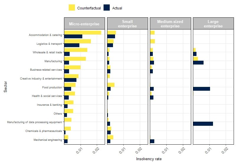

The COVID-19 Insolvency Gap:

                First-round Effects of Policy Responses on SMEs

                   Julian Oliver Dörr∗1,2 , Simona Murmann1 , and Georg Licht1

1
    Centre for European Economic Research (ZEW), Department of Economics of Innovation and Industrial
                                        Dynamics, Mannheim, Germany
           2
               Justus-Liebig-University, Department of Econometrics and Statistics, Gießen, Germany

                                              January 1, 2021

             Abstract COVID-19 placed a special role to fiscal policy in rescuing compa-
          nies short of liquidity from insolvency. In the first months of the crisis, SMEs
          as the backbone of Europe’s real economy benefited from large and mainly
          indiscriminate aid measures. Avoiding business failures in a whatever it takes
          fashion contrasts, however, with the cleansing mechanism of economic crises:
          a mechanism which forces unviable firms out of the market, thereby reallo-
          cating resources efficiently. By focusing on firms’ pre-crisis financial standing,
          we estimate the extent to which the policy response induced an insolvency
          gap and analyze whether the gap is characterized by firms which had already
          struggled before the pandemic. With the policy measures being focused on
          smaller firms, we also examine whether this insolvency gap differs with respect
          to firm size. Based on credit rating and insolvency data for the near universe
          of actively rated German firms, our results suggest that the policy response to
          COVID-19 has triggered a backlog of insolvencies in Germany that is partic-
          ularly pronounced among financially weak, small firms, having potential long
          term implications on economic recovery.

          Keywords: COVID-19 policy response, Corporate bankruptcy, Cleansing effect, SMEs

          JEL:           C83, G33, H12, O38

      ∗
     To whom correspondence should be addressed. E-mail: julian.doerr@zew.de
Acknowledgements: This paper extends upon a project analyzing the economic effects on SMEs in
the COVID-19 crisis which was funded by the German Federal Ministry of Economic Affairs (BMWi)
under the grant agreement No 15/20. In addition, we gratefully acknowledge research funding from the
European Union Horizon 2020 Research and Innovation Action for the ‘GrowInPro’ project under grant
agreement No 822781. The authors thank Dennis Nierychlo for valuable research assistance and Tobias
Weih for comments that greatly improved the manuscript. The views expressed in this paper are those of
the authors and do not necessarily represent the views of the institutions with which they are affiliated.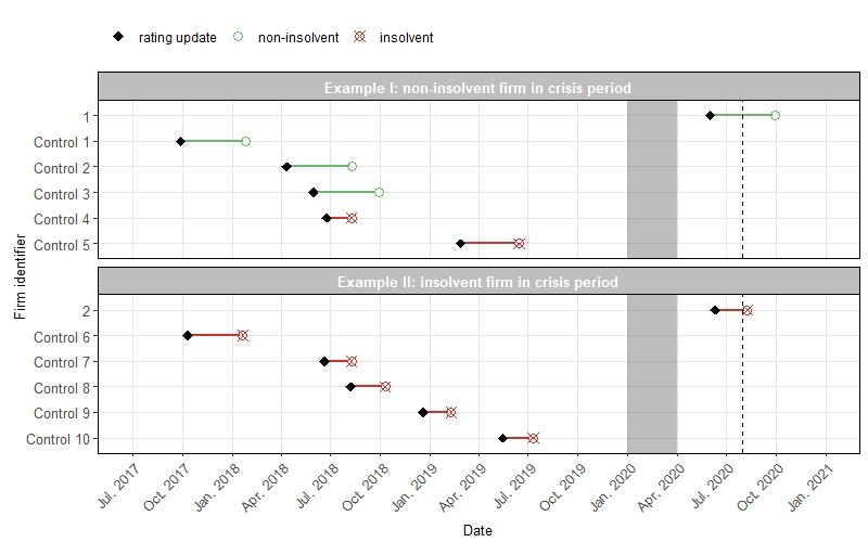

1. Introduction

COVID-19 and its unprecedented economic impacts have ground economies worldwide to

a halt. With the early lockdown measures in place to contain the spread of the virus,

many firms faced a situation of reduced business activity and declining sales, which had

immediate consequences on their liquidity positions. Both the negative demand shock

paired with a negative supply shock in most industries have indeed brought numerous

firms under strong pressure in keeping their operations alive. Previous crises have taught

that smaller companies are particularly prone to considerable liquidity constraints in deep

recessions. For example, literature on the financial crisis of 2007–2009 shows that espe-

cially small and entrepreneurial enterprises were exposed to severe liquidity shocks due to

the collapse of the interbank market and its negative impact on corporate lending (Iyer et

al. 2014; McGuinness and Hogan 2016). While in the Great Recession a large contraction

in corporate lending caused a severe liquidity squeeze in the real economy hitting smaller

firms disproportionately hard (Buckley 2011), the major impact of the combined negative

supply and demand shock in the COVID-19 crisis is also characterized by a deep liquidity

shock in the real sector. Drop of trading activities and lack of business revenues made

many firms dependent on their cash reserves in order to meet their unchanged fixed cost

obligations. As smaller companies are characterized by strong dependence on internally

generated funds to capitalize their business and provide the liquidity needed to finance

day-to-day operations, both their cash reserves and collateral for external financing are

generally limited (Cowling et al. 2011). In times of financial distress as in the current

COVID-19 crisis, this makes small ventures particularly vulnerable candidates for finan-

cial insolvency. Trapped in a situation of thin financial reserves and lack of collateral for

drawing new credit lines, small businesses face therefore a particularly high risk of business

failure without the relief through policy intervention.

  Conscious of the far-reaching consequences of systematic business failures, governments

in almost all countries have initiated a series of emergency measures to strengthen liquidity

positions of their national companies (International Monetary Fund 2020), some of which

exclusively focusing on the relief of Small and Medium-sized Enterprises (SMEs) (OECD

2020). In the European Union (EU), for instance, member states’ liquidity support in

                                              1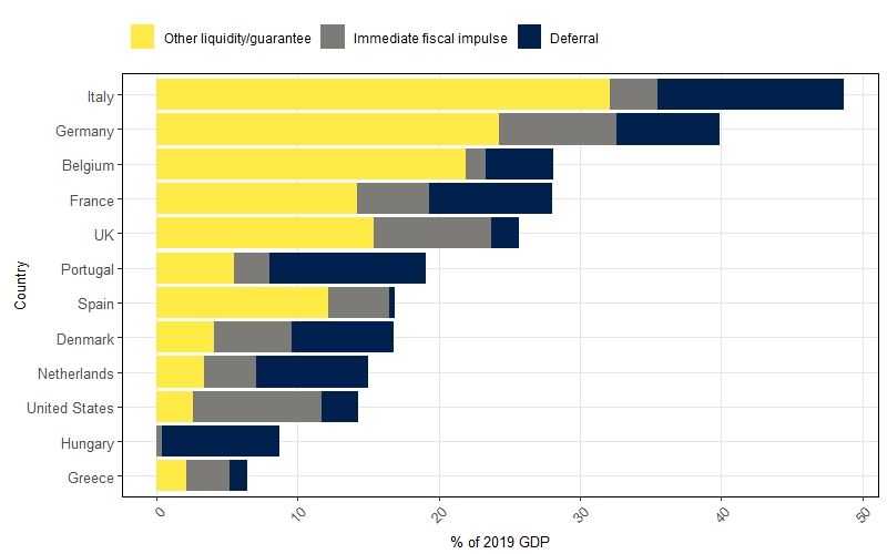

form of public loan guarantees and tax deferrals for distressed sectors has increased by

an estimated 6 percentage points (pp) of EU GDP compared to pre-crisis levels (Council

of the European Union 2020). While fiscal policy measures in most countries have gone

beyond deferrals and loan guarantees, including instruments such as wage subsidies or

adjustments in bankruptcy regimes, these measures were undoubtedly necessary to keep a

struggling economy afloat and avoid large-scale insolvencies. However, since the COVID-

19 crisis required a rapid policy response, it is reasonable to assume that few, if any,

screening mechanisms could be implemented based on firms’ pre-crisis financial position.

Thus, evaluating the viability of firms that received early state aid has been very limited.

In fact, the fast growing literature on business failures in response to the adverse economic

impacts of COVID-19 stresses that the early assistance packages may bare high economic

costs if they keep unviable firms alive (Kalemli-Ozcan et al. 2020; Barrero et al. 2020;

Cowling et al. 2011; Juergensen et al. 2020; OECD n.d.).

     We argue that the early policy measures in most countries were poorly targeted large-

scale interventions to prevent bankruptcies in a ‘whatever it takes’ fashion. Even though

we acknowledge that it is difficult for policy-makers to determine whether a firm’s fi-

nances are strained because of the pandemic or because of other circumstances predating

this crisis, undifferentiated relief measures can be costly in many respects. Kalemli-Ozcan

et al. (2020) provide an early contribution in assessing the costs associated with poorly

targeted policy measures in response to COVID-19. In their analysis, they distinguish

between ‘survivor’, ‘viable’ and ‘ghost’ firms with the latter characterized as companies

which would have failed even without being exposed to the adverse COVID-19 shock. In

their simple cost minimization model, comprising data of 17 European countries, they

find that without proper targeting of policy instruments, the costs of intervention are

substantially higher compared to a scenario in which measures target ‘viable’ firms only

(Kalemli-Ozcan et al. 2020).1

     Despite the direct fiscal costs that come along with undifferentiated policy interventions

there is another source of economic costs associated with keeping unviable firms alive.

In Schumpeterian economics, it may also impede the cleansing effect of creative destruc-
 1
     Moreover, their findings suggest that 19% of ‘ghost’ firms are kept alive in case of undifferentiated
      intervention (Kalemli-Ozcan et al. 2020).

                                                     2

tion (Guerini et al. 2020). The cleansing effect of creative destruction describes a process

in which resources are reallocated from less efficient and less creative firms to more ef-

ficient ones enhancing overall economic productivity and innovation (Schumpeter 1942).

Typically, this process of efficient resource reallocation is particularly strong in times of

economic crisis, allowing viable and innovative firms to gain market share as unprofitable

firms exit the market (Caballero and Hammour 1994; Archibugi et al. 2013; Carreira and

Teixeira 2016). As such, without the intervention of fiscal policy, business failures of un-

viable firms are expected to be substantial in economic recessions and, given the strong

vulnerability of small firms, the effect is expected to be particularly pronounced among

smaller businesses. In the current crisis however, there is growing public concern that this

process of creative destruction and ‘cleaning up’ of unviable firms is seriously hampered

by an increasing policy-induced ‘zombification’ of the economy (see, for example, The

Economist (2020a), Financial Times (2020), The Japan Times (2020), The Washington

Post (2020)). Even though we do not want to go as far as speaking of a zombification,

we still hypothesize that the first-round policy measures with strong focus on SME relief

induced a serious insolvency gap, defined as backlog of corporate insolvencies which are

usually to be expected in a crisis such as this. Looking at corporate insolvency numbers

after the outbreak of the crisis for selected countries, it becomes indeed apparent that in-

solvencies strongly decreased compared to 2019 levels (see Appendix A). The observation

that bankruptcy filings are lower in an economic crisis than in non-crisis times appears

counter-intuitive at first and underpins that the large-scale governmental support pro-

grams have led to substantial distortions.

  Making use of unique credit rating and insolvency data, the central purpose of this

paper is to analyze whether indeed such an insolvency gap exists and by which companies

it is mainly driven. Our hypothesis is that the risk of unviable ‘survivors’ is particularly

severe among mainly small and micro companies as they tend to be particularly prone to

liquidity shortages in times of crises and therefore benefit most from state support com-

pared to a situation in which the policy maker does not step in. The strong policy focus

on SMEs reinforces this hypothesis (OECD 2020). Finally, the prolonged expansion prior

to the COVID-19 pandemic and the low interest rate environment suggest that a signifi-

cant number of financially weak companies that were already on the brink of bankruptcy

                                             3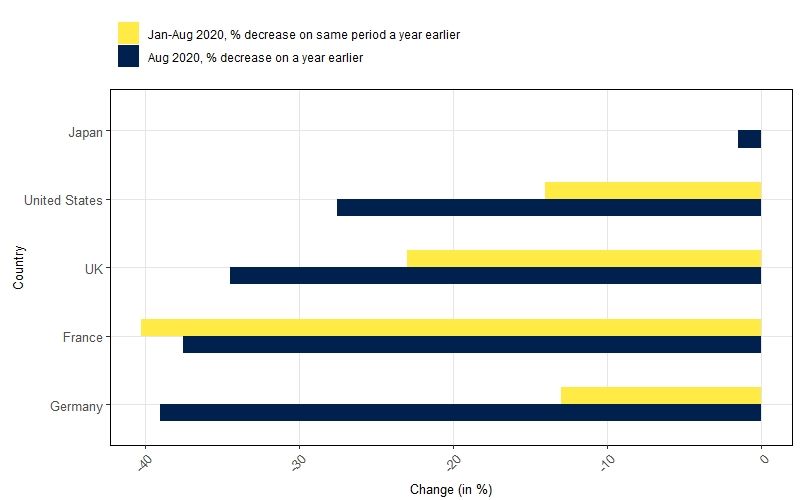

before the onset of the crisis have accumulated over time (Barrero et al. 2020). Given this

interplay between prolonged expansion and sudden economic decline with strong policy

response, it is likely that the insolvency gap is driven by firms with weak financial pre-crisis

conditions.

     Our contribution to the fast growing literature on the economic effects of the COVID-

19 crisis is manifold. First, we examine the heterogeneity with respect to firm size in

policy makers’ response to the risk of large-scale business failures. By doing so we focus

on Germany, a country where SME state support is particularly strong by international

comparison (Anderson et al. 2020; OECD 2020). Building on Schumpeter’s theory of

the cleansing effect in economic crises, undifferentiated first-round policies in the current

crisis may have favored unviable firms to stay in the market, hampering the release and

efficient reallocation of resources. We transfer this theoretical concept into an empirical

assessment by estimating a COVID-19-induced insolvency gap using firm-specific credit

rating data combined with information on insolvency filings. Controlling for updates in

a firm’s credit rating, we estimate insolvency rates after the COVID-19 outbreak in a

counterfactual setting of no policy intervention. Comparable firms with closely matching

changes in their credit rating in non-crises times are used as control group. Hence, we

estimate the insolvency gap induced by COVID-19-related policy measures using a po-

tential outcome setting. As the COVID-19 pandemic hits sectors asymmetrically2 and

policy measures were relatively more generous to micro and SMEs businesses3 , we con-

duct the insolvency gap estimation at the sector-size-level. Unlike Kalemli-Ozcan et al.’s

(2020) work, our contribution builds upon a representative sample with respect to firm

size allowing a nuanced differentiation between medium-sized, small and micro-enterprises.

     The remainder of the paper proceeds as follows. In Section 2 we discuss the fiscal policy

responses to the COVID-19 outbreak in Germany emphasizing their different focus with

respect to firm size. Section 3 introduces the data sources and variables used to estimate

the insolvency gap. Moreover, the matching framework for the matching of counterfac-

 2
   See Section 4.1 for a survey-based examination of the negative economic impacts of the pandemic on
    German firms controlling, among other factors, on the firms sector affiliation. The results suggest
    heterogeneous effects across sectors.
 3
   See Section 2 for an assessment how state response to the COVID-19 crisis differs with respect to firm
    size.

                                                   4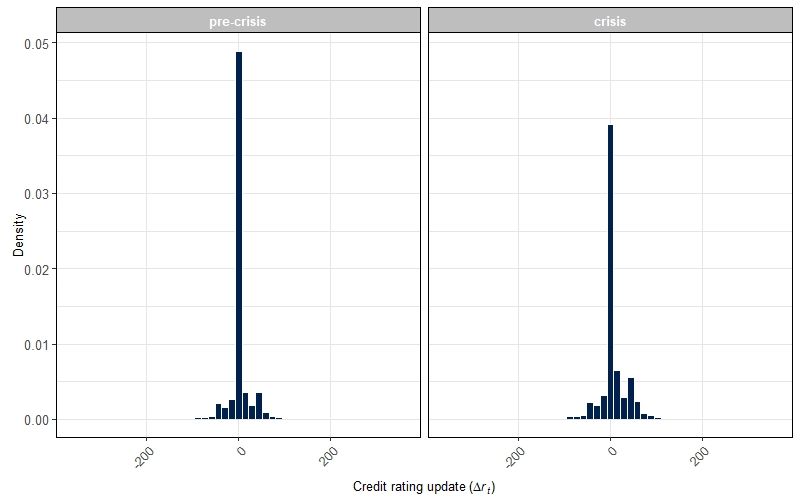

tual survival states is introduced. Section 4 empirically examines the heterogeneity of

the economic effects of the COVID-19 pandemic across firms of different size and sector

affiliation. Ultimately, it presents the empirical results of the insolvency gap estimation

and discusses its implications. Section 5 concludes.

2. Fiscal policy response in Germany

Official figures show that in Germany, the fiscal policy response to prevent corporate in-

solvencies due to crisis-related liquidity bottlenecks is particularly pronounced by interna-

tional comparison. According to a comparative study of the economic think tank Bruegel

analyzing the fiscal response to the economic fallout from the pandemic, nearly 40% of

Germany’s 2019 GDP was spent on COVID-19 measures to strengthen companies’ liquid-

ity positions (Anderson et al. 2020). Compared with a number of selected Organization of

Economic Cooperation and Development (OECD) countries, this is the second strongest

response in terms of a country’s overall economic performance (see Figure 1). The Ger-

man Federal Government itself describes the response as the ‘largest assistance package in

the history of the Federal Republic of Germany’ (Federal Ministry of Finance 2020d, p. 3).

  From a small business economics view it is interesting to see that many of the in-

tervention measures adopted by the German Federal Government have been specifically

designed to target SMEs (OECD 2020). For example, in immediate response to the early

lockdown measures, the government granted one-off cash injections for self-employed per-

sons and micro-businesses with up to 10 employees (‘Soforthilfen’) in form of a stimulus

package worth e50 billion (Federal Government of Germany 2020). These immediate sub-

sidies have been accompanied by the provision of loans from Germany’s government-owned

promotional bank KfW for which the government assumes 100% of the credit risk (‘KfW-

Schnellkredite’). The volume of the loan program and the related government guarantees

are potentially unlimited and they were designed to improve liquidity positions especially

of SMEs (Federal Ministry of Finance 2020d). Moreover, as part of a large-scale stimulus

package worth e25 billion, SMEs that had to cease or severely restrict their business op-

erations in the wake of the COVID-19 pandemic have become eligible for state-financed

liquidity support (‘Überbrückungshilfen’) covering a substantial part of their fixed oper-

                                             5

Figure 1 COVID-19 fiscal policy response by international comparison

Note: Calculations are retrieved from Anderson et al. (2020). Numbers reflect the amount (as share of
2019 GDP) of policy measures to address adverse COVID-19 impacts on companies for selected OECD
countries. Numbers are as of by 18 November 2020.

ating costs (Federal Ministry of Finance 2020c). In the following, we describe the fiscal

policy instruments to counter the economic impacts of the COVID-19 crisis in more detail,

focusing on how the instruments differ with respect to firm size.

Liquidity subsidies and government guarantees

The most important instrument is the provision of liquidity, either through direct cash

transfers like the aforementioned ‘Überbrückungshilfen’ or through loans backed by public

guarantees. The extent of liquidity support is primarily determined by company size,

measured by the number of employees or previous revenues. In case of the one-off grants,

for instance, only micro-firms with up to 10 employees were eligible to receive injections

between e9,000 and e15,000 for three months to cover their operational costs (Federal

Ministry of Finance 2020d). This support was granted in a non-bureaucratic fashion easily

accessible to all micro-businesses which assured that they were suffering financial distress

as a result of the COVID-19 pandemic (Federal Government of Germany 2020).

  For SMEs with more than 10 employees the KfW Instant Loan Program has been

launched. The program offers SMEs loans that are fully collateralized by the state. These

                                                 6

loans amount up to 25% of a firm’s 2019 revenues with a cap of e500k for small companies

and e800k for medium-sized companies, respectively. No credit risk assessments are taking

place and no collaterals are required. The only eligibility criterion is that the company

was profitable in 2019 or at least on average profitable between 2017 and 2019 (Federal

Ministry for Economic Affairs and Energy 2020). This fairly broad criterion shows that

the process is focused on speed and ease applied ‘without red tape’ Federal Ministry of

Finance (2020b, p. 1) and not on elaborate screening mechanisms that could prevent

providing liquidity to unviable firms.

  Furthermore, the COVID-19 support package includes additional government guarantees

on loans for both small and larger businesses. Similar to the Instant Loan Program, the

loans are channeled through commercial banks and the state-owned bank KfW assumes

risk coverage of 80% for large enterprises and 90% for SMEs with a highly simplified risk

assessment (Federal Ministry of Finance 2020a). In addition, interest rates are lower for

SMEs than for large firms (Federal Ministry for Economic Affairs and Energy 2020). This

makes lending to SMEs particularly attractive for commercial banks and, given that they

only bear 10% of the risk, further reduces the need for a comprehensive risk assessment.

Short-time work (STW) scheme

Another form of liquidity support to companies is the use of short-time compensations

(‘Kurzarbeitergeld’) which are direct subsidies on firms’ labor costs. This instrument

has been available for quite some time; however, it’s eligibility criteria were relaxed in

the pandemic. Now companies with only 10% of employees being on STW qualify for

a wage subsidy (instead of one third) (OECD n.d.). In addition, the subsidy has been

increased compared to pre-crisis levels, ranging now from 60% to 87% of the worker’s

last net income. From the company’s perspective, short-time compensations reduce labor

costs, allow the company to retain specific human capital and avoid the costs of new

hires and training when the economy recovers again. Drawing on literature from the

Great Recession, the usage of STW has a positive impact on firm survival (Cahuc et al.

2018; Kopp and Siegenthaler 2020) but at the same time low productivity firms have been

much more likely to take up STW (Giupponi and Landais 2018, 2020). From a welfare

perspective, this may have adverse effects as it impedes the reallocation of workers from

low- to high-productivity firms. Moreover, SMEs tend to be active in more labor-intense

                                            7

business activities than larger firms (Yang and Chen 2009). Therefore, it is reasonable to

assume that SMEs as well as labor-intense sectors benefit disproportionately from short-

time compensations. Since the eligibility criteria for STW are unrelated to firms’ pre-crisis

performance, also unviable companies benefit from the instrument.

Tax deferrals

To further improve the liquidity situation of companies, authorities have granted tax

payment deferrals, allowed lower tax prepayments and suspended enforcement measures

for tax debts. The tax-related assistance amounts to an estimated e250 billion and the

policy measure applies equally to all company size classes (Anderson et al. 2020).

Temporary change in insolvency law

Finally, the Federal Government enacted a temporary amendment to the German insol-

vency law that is closely related to the possible existence of a policy-induced insolvency

gap. On March 27, 2020, it decided to temporarily suspend the insolvency filing obligation

in order to avoid a massive increase in insolvencies as a result of COVID-19-induced liq-

uidity shortages. The obligation to file an insolvency has been suspended until September

30th, 2020, with an adjusted extension until the end of 2020. This suspension enables both

small and large companies to avert insolvency and possibly survive the crisis by taking ad-

vantage of state aid (Federal Ministry of Justice and Consumer Protection 2020). Although

the amended law stipulates that only those firms that are insolvent or over-indebted due

to the COVID-19 pandemic are temporarily exempt from insolvency proceedings, policy

makers face the dilemma that it is barely possible to assess whether insolvent non-filers

fulfill these eligibility criterion. This is particularly true for smaller firms, whose limited

disclosure requirements make such an assessment even harder. While there is no doubt

that many viable companies facing illiquidity and over-indebtedness as a result of the eco-

nomic shock will benefit from the change in the law, it also creates loopholes for smaller,

non-viable companies to stay in the market and absorb liquidity subsidies.

  This section has highlighted the role of fiscal policy to counter the economic conse-

quences of the pandemic in Germany - a country that has provided substantial assistance

to businesses to avoid large-scale bankruptcies. While the suspension of the insolvency

                                              8

filing requirement is the driving force behind our assumption of an existing insolvency gap,

direct and indirect liquidity subsidies are likely to work in the same direction. Especially

for companies that do not meet the eligibility criteria for the insolvency exemption, the

provision of liquidity by the state can nevertheless save ailing companies from failure. It

has been shown that many of the policies directly target SMEs or provide indirect channels

for small businesses to benefit disproportionately. This comes at the potential risk that

unviable firms are kept alive, ultimately leading to a possible backlog in insolvencies which

is likely to be particularly pronounced among SMEs. In the next section, we introduce the

data and methodology we use to estimate the existence and extent of such an insolvency

gap.

3. Data, variables and methodology

3.1. Data and variables

The study makes use of two data sources which both originate from the Mannheim En-

terprise Panel (MUP) covering the near universe of economically active firms in Germany

(Bersch et al. 2014). The first data source is a survey where the questioned companies have

been sampled from the MUP. The survey is used to examine how companies of different

size and in different sectors are affected by the adverse impacts of the COVID-19 pandemic

and motivates why we estimate the insolvency gap distinguishing between sector affiliation

and company size. For the estimation of the insolvency gap we use a second data source:

a large sample of firm-specific credit rating information along with information concerning

the firms’ insolvency status. In the following, we will introduce both data sets and the

variables used in this study in more detail.

3.1.1. Survey data

We employ the survey to primarily assess which industries and company sizes are affected

most by the crisis.4 Based on a representative random sample of German companies,

drawn from the MUP and stratified by firm size and industry affiliation5 , the survey was

conducted three times spanning the period in which the German insolvency regime was
 4
   The survey has been conducted as part of a joint research project between the German Federal Ministry of
    Economic Affairs (BMWi), the polling agency Kantar and the Centre for European Economic Research
    (ZEW).
 5
   Table 2 shows the stratification criteria used in the subsequent analysis.

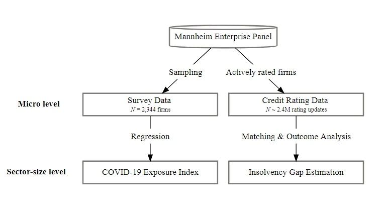
                                                    9

Figure 2 Data sources used in this study

Note: Observations of the survey data (companies) and credit rating data (firm-specific rating revisions)
originate from the Mannheim Enterprise Panel (MUP) data base. Survey data allows to estimate exposure
to adverse effects of the pandemic on the sector-size level. Credit rating data is used to estimate the
existence of an insolvency gap on the sector-size level.

fully suspended.6 The survey includes questions on COVID-19-related economic effects on

various business dimensions. The collected data has then been supplemented with credit

rating scores from the MUP, which allows to control for the financial situation of the

companies prior to the crisis. As shown in Figure 2, we use the survey data to investigate

whether the adverse economic impacts of COVID-19 differ across sectors and firm size

classes. These results together with the heterogeneity in public aid programs with respect

to firm size as outlined in Section 2 motivates us to conduct our main empirical analysis

at the sector-size level.

     Table 1 shows summary statistics of the relevant variables used to construct a COVID-19

Exposure Index, CEI, reflecting the extent to which firms experienced negative impacts

in relation to the pandemic. Firms were asked on a Lickert scale of 0 to 4 in which of the

following areas they experienced negative impacts as a result of the COVID-19 crisis: (1)

decrease in demand (2) shutdown of production (3) supply chain interruption (4) staffing

shortage (5) logistical difficulties (6) liquidity shortfalls.7 From these six questions we
 6
   The surveys have been conducted in April 2020, in June 2020 and in September 2020 spanning the period
    of the full suspension of the obligation to file for insolvencies and is therefore particularly suitable for
    capturing the policy induced effects of the crisis.
 7
   0 indicates no negative effects, 4 signals strong negative effects.

                                                      10

construct CEI as simple sum of the response values. The average index is 6.312 out of

a maximum possible value of 24. The most common and most severe impact relates to

the decline in demand, where respondents reported an average negative impact of 1.851.

Shutdown of production facilities and liquidity bottlenecks are also frequently mentioned

consequences. Table 1 also displays size and sector dummies which will later be used as

stratification criteria in the estimation of the insolvency gap.

Table 1 Descriptive statistics: Survey data
 Variables                                                    N        Mean           SD       Min     Max
 COVID-19 Exposure Index (CEI)                              2,344       6.312       5.397         0      24
 Questions used for COVID-19
 Exposure Index calculation
 (1) Decrease in demand                                     2,344       1.851       1.556         0        4
 (2) Lockdown of production                                 2,344       1.048       1.583         0        4
 (3) Supply chain interrupted                               2,344       0.875       1.236         0        4
 (4) Staffing shortage                                      2,344       0.639       1.044         0        4
 (5) Logistical difficulties                                2,344       0.813       1.277         0        4
 (6) Liquidity shortfalls                                   2,344       1.084       1.414         0        4
 Size of company
 Micro-enterprise                                           2,344       0.394       0.489         0        1
 Small enterprise                                           2,344       0.300       0.459         0        1
 Medium-sized enterprise                                    2,344       0.204       0.403         0        1
 Large enterprise                                           2,344       0.102       0.302         0        1
 Sector affiliation
 Mechanical engineering                                     2,344       0.081       0.273         0        1
 Chemicals & pharmaceuticals                                2,344       0.058       0.235         0        1
 Data processing equipment                                  2,344       0.061       0.241         0        1
 Food production                                            2,344       0.071       0.258         0        1
 Other manufacturing industries                             2,344       0.121       0.326         0        1
 Wholesale & retail trade                                   2,344       0.112       0.316         0        1
 Accommodation & catering                                   2,344       0.060       0.239         0        1
 Insurance & banking                                        2,344       0.063       0.243         0        1
 Creative industry & entertainment                          2,344       0.061       0.240         0        1
 Other business-related services                            2,344       0.140       0.347         0        1
 Health and social services                                 2,344       0.095       0.293         0        1
Note: Table shows descriptive statistics of the COVID-19 Exposure Index (CEI). It also displays statis-
tics of the survey questions used to construct the index. Ultimately, the size and sector distribution in the
survey data is shown.

3.1.2. Credit rating data

For the purpose of estimating whether the bankruptcy filing behavior has changed sig-

nificantly as a result of the crisis-related aid measures and possibly created a backlog of

                                                     11

insolvencies, we examine credit rating updates of close to all economically active firms

listed in the MUP.8 The Mannheim Enterprise Panel is particularly suited for an analysis

of the insolvency-related cleansing effect as it is constructed by processing and structur-

ing data collected by Creditreform, the leading credit agency in Germany. Creditreform

regularly measures and updates the creditworthiness of German companies. Overall our

sample comprises 2,373,782 credit rating updates of 1,500,764 distinct German businesses

whose ratings were updated at least once during the last three years.9 Table 2 shows that

the sample of about 1.5 million companies is very diverse in its industry and size compo-

sition. Most important in the context of this study is the coverage of SMEs, which is not

only representative for the German economy (Destatis 2020), but also allows for a nuanced

differentiation between medium-sized, small and micro-enterprises. Therefore, it suits well

to examine the policy-induced heterogeneity of the COVID-19 related effects on business

failures with a special focus on possible size differences not only among SMEs and large

enterprises but also within the group of SMEs. The latter estimation of the insolvency

gap will be conducted on the sector-size level as displayed in Table 2 comprising S = 52

distinct sector-size strata.

     Assuming that the COVID-19 shock and its economic consequences on liquidity and

insolvency distress of German businesses began by the end of March 2020, we split our

sample into a ‘pre-crisis’ period and a ‘crisis’ period. This cut-off point also captures

COVID-19 policy dynamics as the German government imposed the first countrywide

lockdown that includes a shutdown of most customer service-related businesses on March

22 and suspended the obligation to file for bankruptcy on March 27 (Federal Ministry

of Justice and Consumer Protection 2020). Consequently, the pre-crisis period comprises

all credit rating updates which took place between July 2017 and December 2019. The

crisis period includes all observations between April 2020 and end of July 2020.10 In the

later estimation of the insolvency gap, rating updates from the pre-crisis period serve as

pool of control observations. Closely matching credit rating updates from this pool are

 8
   In our analysis a company is defined as economically active if it has received a credit rating update at
    least once over the last three years spanning the period from July 2017 to July 2020.
 9
   We observe one and the same company at most three times in our sample. Thus, credit rating updates
    normally do not take place more often than once per year but may be conducted in a less regular cycle.
10
   Note that we exclude observations between January 2020 and March 2020 which we see as transitional
    phase in which assignment to either of the two periods is not straightforward. Also note that July 2020
    is the latest month for which we observe credit rating information.

                                                   12

Table 2 Sample decomposition of credit rating data
                                                              Size of company                            Total
 Sector affiliation
                                                      Micro      Small     Medium        Large         (sample)

 Business-related services                             89.4%       8.3%        1.9%        0.4%         28.6%
 Manufacturing                                         84.9% 11.8%             2.7%        0.6%         22.5%
 Wholesale & retail trade                              83.1% 13.4%             2.9%        0.6%         19.9%
 Health & social services                              84.8% 10.6%             3.5%        1.1%           7.3%
 Insurance & banking                                   93.6%       3.6%        1.8%        1.0%           4.5%
 Accommodation & catering                              88.5%       9.8%        1.6%        0.1%           4.1%
 Logistics & transport                                 80.5% 15.3%             3.5%        0.7%           4.1%
 Others                                                82.7% 10.2%             4.6%        2.5%           3.9%
 Creative industry & entertainment                     88.9%       8.8%        2.0%        0.3%           1.6%
 Mechanical engineering                                54.3% 27.5%            13.0%        5.2%           1.3%
 Food production                                       64.3% 23.0%            10.3%        2.4%           1.0%
 Chemicals & pharmaceuticals                           49.1% 29.1%            16.5%        5.3%           0.7%
 Manufacturing of data processing                      58.9% 26.7%            10.9%        3.5%           0.5%
 equipment
 Total (sample)                                        85.2% 11.1%             2.9%        0.8%          100%

 Total (population)a                                   81.8% 15.1%             2.5%        0.6%          100%
Note: Table shows the company size distribution within sectors (rows) as well as the sector distribution
(column ‘Total (sample)’) in our credit rating sample. Size classification is determined by number of em-
ployees, annual turnover and annual balance sheet total following the recommendation of the EU Commis-
sion (European Commission 2003) as outlined in Appendix B. Sector groups are built to reflect anecdotal
heterogeneity in the context of COVID-19. Grouping of sectors is based on EU’s NACE Revision 2 clas-
sification scheme (European Union 2006). In Appendix C an exact mapping of sector groups and NACE
divisions can be found. In all sectors the fraction of SMEs lies far above 90% which makes the data par-
ticularly useful to analyze the effects of COVID-19-related policy responses on smaller firms. Also note
that the overall size composition of our sample compares well against the official size distribution of the
population of German active companies as reported by the Federal Statistical Office (Destatis 2020).
a
  Population size distribution according to official statistics of the Federal Statistical Office (Destatis 2020).

used to estimate counterfactual insolvency rates which will be compared against the actual

insolvency rates observed after April 1, 2020.11

     For the estimation of insolvency rates, we enrich our sample of firm-specific credit rating

data with information on the firm’s survival status after it has received an update on its

rating. Information on firm-specific survival states is obtained by the online register for

bankruptcy filings of the German Ministry of Justice. Besides information identifying the

companies which have filed for insolvency, the register also contains the filing date, allowing

11
     Figure 3 provides an illustration of how closely matching observations from the pre-crisis period serve
      as controls for rating changes of firms in the crisis period.

                                                       13

us to match the most recent rating update that predates the filing date for that particular

bankrupt firm. Our overall sample comprises 15,634 credit rating updates that were fol-

lowed by an insolvency and 2,358,148 rating updates which did not result in an insolvency

filing. With this data, we are able to estimate two statistics. First, we use this information

to estimate bankruptcy rates after the COVID-19 outbreak on the sector-size-level based

on firms for which we observe credit rating updates during the pandemic. Second, using

comparable firms with closely matching credit rating updates in non-crises times as control

group, we are able to estimate counterfactual insolvency rates also on the sector-size-level.

Comparing observed insolvency rates with counterfactual insolvency rates within each of

the sector-size strata allows us to obtain sector-size-specific estimates of the insolvency

gap. In addition to firm size, industry affiliation, and credit rating update, we consider an

extensive set of additional firm-specific variables when matching counterfactual survival

states of pre-crisis observations with rating updates of firms observed in the COVID-19

period. In the following section, we introduce all of these matching variables and provide

some descriptive statistics.

  In our data used for the estimation of the insolvency gap firm survival status, ft+4 ,

serves as outcome variable. It is equal to 1 if the company has filed for insolvency no

more than four months after its last rating update. If the firm has not gone bankrupt or

it has filed insolvency more than four months after its latest rating update, it takes on

the value 0. This means that we take four months as maximum time lag between a credit

rating update and the date at which the respective firm has filed its bankruptcy to count

the rating update as being predictive for the subsequent insolvency filing. We choose this

threshold for two reasons. First, we want to ensure that the rating update has a high

information content in predicting a potential insolvency filing. If the date of bankruptcy

lies more than 4 months after the credit update, it is likely that the update does not reflect

the reasons why the company went bankrupt. A more recent update of the firm’s rating

(if that existed) would be necessary to capture the company’s financial deterioration that

contributed to the subsequent insolvency. Second, the COVID-19 period for which we

have information on credit rating updates spans 4 months from April 2020 to the end of

July 2020. Thus, for the latest in-crisis rating updates in July 2020, we can observe the

firm’s survival status at most 4 months until November 2020 (the time of writing this

                                             14

paper). Therefore, the maximum forecasting horizon for the rating updates observed in

the crisis period is limited to 4 months.

     The most important variable in finding counterfactual survival states in the matching

procedure is Creditreform’s credit rating index since it is the basis for the calculation of the

credit rating updates. The credit rating is calculated by Creditreform on the basis of a rich

information set relevant to assess a company’s creditworthiness. The metrics considered

in calculating the rating include, among other things, information on the firm’s payment

discipline, its legal form, credit evaluations of banks, credit line limits and risk indicators

based on the firm’s financial accounts (if applicable) (Creditreform 2020b). Creditreform

attaches different weights to these metrics according to their relevance on determining

a firm’s risk of credit default and calculates an overall credit rating score which ranges

from 100 to 500.12 The higher the score, the worse the firm’s creditworthiness and thus

the higher the risk of insolvency. In fact, Creditreform’s solvency index has a high fore-

casting quality to assess a firm’s credit default risk (Creditreform 2020b). Assuming that

a high credit default risk signals financial distress, which often results in insolvency, we

use Creditreform’s credit rating as the basis for predicting corporate insolvency risk. The

prediction of corporate bankruptcy via a scoring model goes back to the seminal work

of Altman (1968) and his development of the Z-score model. Similar to Creditreform’s

credit rating index, the Z-score model relies on several accounting-based indicators which

are weighted and summed to obtain an overall score. This score then forms the basis for

classifying companies as insolvent or non-insolvent (Altman 2013). Today, this model ap-

proach is still used by many practitioners to predict firm insolvencies (Agarwal and Taffler

2008).

     Based on the credit rating index, we construct the following variables. Our main predic-

tor variable is the update in the rating index, ∆rt , which is defined as the difference of the

new rating assigned by Creditreform an the rating before the update (∆rt = rt − rt−x ).13

Given the logic of the rating index, a positive sign in the rating update reflects a down-
12
   The credit rating index suffers from a discontinuity as in case of a ‘insufficient’ creditworthiness it takes
    on a value of 600 (Creditreform 2020a). We truncate credit ratings of 600 to a value 500 - the worst
    possible rating in our analysis. We do so since our main predictor variable is the update in the rating
    index which can only be reasonably calculated if the index has continuous support.
13
   Reassessments of the rating is conducted in an irregular fashion such that the time between two updates,
    x, varies. On average, the time between two updates equals 20 months.

                                                      15

grade in financial solvency, a negative sign reflects an improvement in the rating, i.e. an

upgrade of the company’s financial standing. The amount of the down-/upgrade reflects

how severely the company’s financial standing has changed.14

     Apart from the rating update, we also consider the rating before the upgrade, rt−x , as

a matching variable when predicting counterfactual insolvency states. This allows us to

control for where the company is located in the rating distribution and consequently how

high the default risk was before the down-/upgrade. Moreover, we form two additional

variables from the firm’s credit rating information, both of which control for the medium-

term path of the firm’s financial standing. First, we count the number of downgrades in

the three years preceding the update at hand, dt . Second, we calculate the average credit

rating in the three years prior to the current update under consideration, r̄t .15 Finally, we

consider firm age, at , as further matching variable acknowledging that younger firms tend

to be more prone to insolvency.

     Table 3 shows descriptive statistics of the variables considered in the matching pro-

cedure. We see that an update which is followed by a bankruptcy filing relates to a

downgrade of close to 70 scoring points on average. This is a substantial deterioration

in the rating index compared to an update which is not followed by an insolvency filing.

In fact, the difference in means between non-insolvency-related updates and insolvency-

related updates, as reported in column ‘∆ Mean’, amounts to more than 65 index points

and is statistically significant. For all other matching variables, we also find statistically

meaningful differences suggesting that firms which go bankrupt have a worse credit rat-

ing both short-term and mid-term, have experienced more downgrades in the past and

are younger on average. The economically and statistically significant differences between

non-insolvency-related and insolvency-related credit updates across all variables suggest

that they serve well as matching variables in a counterfactual estimation of insolvency

14
   Note that we define a rating update as a reassessment of the company’s creditworthiness performed by
    Creditreform. We have precise information on the date of reassessment, which allows us to accurately
    assign the update to either the pre-crisis or the crisis period and also to accurately match the updates
    with insolvency dates. It should also be noted that a reassessment does not necessarily lead to a change
    in the rating index. If the creditworthiness of the company has not changed since the last rating, the
    company gets assigned the same index as before, resulting in a value of 0 in ∆rt .
15
   For example, for a credit rating observation in July 2017, we count how often the firm experienced a
    downgrade over the period June 2014 to June 2017 and also calculate the average rating over that
    period.

                                                    16

rates.

         17

Table 3 Descriptive statistics: Non-insolvent observations & insolvent observations
                                                                   non-insolvent                                              insolvent
                                                                                                                                                                 ∆ Mean
         Variable
                                                    N          N firms       Min      Mean         Max        N       N firms      Min         Mean       Max
      Predictor variables
        Credit rating update: ∆rt               2,358,148     1,489,376     -356       4.0099       351    15,634      15,634      -226        69.6892    359 −65.6793***
        Credit rating (prior to                 2,358,148     1,489,376      100     266.5879       500    15,634      15,634       141       414.6607    500 −148.0728***
        update): rt−x
        Number of downgrades                    2,358,148     1,489,376         0      0.4797          3   15,634      15,634         0         0.5051      3      −0.0254***
        (3-year horizon): dt
        Average credit rating (3-year           2,358,148     1,489,376      100     265.8216       500    15,634      15,634       138       367.6691    500 −101.8475***
        horizon): r̄t
        Company age: at                         2,346,686     1,479,383         1     22.2604     1,017    15,166      15,166         1        13.3199    400         8.9405***
     Note: Non-insolvent observations comprise credit rating updates which have not resulted in an insolvency filing in the first four months after filing. Insolvent observations
     include observations which have been followed by an insolvency filing in the first four months after filing. N refers to the number of rating updates, N f irm to the number of
     unique firms which experienced at least one rating update. Significance levels: *: p < 0.10, **: p < 0.05, ***: p < 0.01

     Table 4 Descriptive statistics: Pre-crisis observations & crisis observations
18

                                                                      pre-crisis                                                    crisis
                                                                                                                                                                       ∆ Mean
         Variable
                                                    N          N firms       Min      Mean         Max         N        N firms     Min         Mean            Max
      Outcome variable
       Survival status: ft+4                    2,036,103     1,377,671         0      0.0071          1   337,679      337,679           0      0.0033           1      0.0038***
      Predictor variables
        Credit rating update: ∆rt               2,036,103     1,377,671     -356       3.9825       359    337,679      337,679     -293         7.2161         349    −3.2336***
        Credit rating (prior to                 2,036,103     1,377,671      100     267.5344       500    337,679      337,679      100       267.7361         500    −0.2017**
        update): rt−x
        Number of downgrades                    2,036,103     1,377,671         0      0.4812          3   337,679      337,679           0      0.4714           3      0.0098***
        (3-year horizon): dt
        Average credit rating (3-year           2,036,103     1,377,671      100     266.3589       500    337,679      337,679      100       267.2973         500    −0.9384***
        horizon): r̄t
        Company age: at                         2,024,173     1,367,244         1     22.0970     1,017    337,679      337,679           1     22.8378   1,016.00     −0.7408***
     Note: Pre-crisis period comprises all credit rating observations from July 2017 to December 2019. Crisis period includes all observations starting from April 2020 to July
     2020. Although the mean differences in the predictor variables (except credit rating update) are statistically significant, their magnitude seems to be rather negligible, partic-
     ularly when comparing with the differences between non-insolvent and insolvent observations (Table 3). This suggests that the crisis sample is not biased in the sense that it
     primarily includes credit updates of firms with poor financial records. Significance levels: *: p < 0.10, **: p < 0.05, ***: p < 0.01

We also report univariate descriptive statistics of our credit rating sample differentiating

between the pre-crisis and the crisis period in Table 4. We see that in the period before the

COVID-19 crisis has hit the German economy, 0.71% of rating updates were followed by a

bankruptcy filing. This translates into an insolvency filing rate of 1.05% on the firm level

(note that firms can receive more than one credit rating update in that period). In the

crisis period, however, despite the worsened economic conditions, it turns out that only

0.33% of rating updates were followed by a bankruptcy filing. This fraction also equals the

firm-level insolvency filing rate as in the 4-months crisis period each firm is only observed

once. ‘∆ Mean’ reporting the difference between the variable means of the pre-crisis and

the crisis period suggests that the difference of 0.38 pp in the average survival status is

statistically significant. The lower average insolvency rate in the crisis period contrasts

with the finding that the financial rating of firms observed in the crisis period has deteri-

orated on average. In fact, firms experience, on average, a significantly higher downgrade

of more than three index points during the crisis period.16 This is a first indication that

there may indeed be an insolvency gap in the German economy. Despite the deterioration

in financial solvency, there are fewer bankruptcy filings compared to pre-crisis times. The

strong political reaction to strengthen firms’ liquidity and to prevent German companies

from going bankrupt is likely to be a driving force behind the low insolvency rate.

     It remains to be analyzed if there are specific sector-size combinations for which the

number of insolvencies is significantly below the counterfactual number that one would

expect given the observed rating updates and information from pre-crisis insolvency paths.

Also we aim to tackle the question whether the gap is mainly driven by firms which already

before the crisis were characterized by a weak financial standing. In the next section, we

introduce a matching approach that allows us to predict counterfactual insolvency filings

if there was no policy intervention for the firms for which we observe rating updates during

the crisis. With this approach, we are able to derive counterfactual insolvency rates at the

sector-size level and provide an estimate regarding the existence of an insolvency gap by

comparing them with the actual filings observed during the crisis period.

16
     See also Appendix D for a comparison of the distribution of the credit rating updates in the pre-crisis
      and the crisis period.

                                                      19

3.2. Methodology

3.2.1. Nearest neighbor matching

This paper focuses on the extent to which state aid measures that address the economic

impact of the COVID-19 crisis may have induced ailing firms to stay in the market. To

answer this question, we compare the survival status of closely matching firms observed

before the COVID-19 outbreak with the survival status of firms observed during the pan-

demic. Besides general company characteristics such as company size, industry affiliation

and company age, our matching approach takes particular account of firm-specific sol-

vency information as presented in the previous section. The core idea of the matching

procedure is to find comparable firms which have experienced very similar rating updates

and have followed an almost identical path in their financial solvency but in times prior

to COVID-19 and the related policy interventions that keep struggling firms afloat.

  In order to find for each of the in-crisis observations a number of matches from the

pre-crisis period, we conduct a nearest neighbor matching approach. Nearest neighbor

matching in observational studies goes back to the work of Donald Rubin (Rubin 1973)

and aims at reducing bias in the estimation of the sector-size-specific insolvency gap. A

simple comparison of the mean values of the survival status of observations before the

crisis and during the crisis (as in Table 4) is likely to give a highly biased picture of the

insolvency gap. First, policy measures to rescue firms from failing have been highly het-

erogeneous with respect to firm size as highlighted in Section 2. Therefore, comparing the

survival status of firms of different size bears high risk of firm size acting as confounding

variable in the estimation of a policy-induced backlog of insolvencies. For this reason,

we only search for matches within the same company size group. Next, the evaluation of

our survey suggests that there is great heterogeneity in the COVID-19 exposure across

sectors (see Section 4.1). For this reason, we only match firms that are in the same sector

class. Ultimately, the previous section has shown that in the crisis period the distribu-

tion of rating updates has systematically shifted to the right implying that the in-crisis

observations have, on average, experienced larger downgrades in their ratings. For an

unbiased estimation of the insolvency gap, this shift needs to be controlled for. Our near-

est neighbor matching aligns the in-crisis distribution of updates with the distribution of

                                             20

matched observations as we put a strict caliper on the credit rating variable when searching

for matching observations. In fact, comparing the distribution of the predictor variables

between pre-crisis and crisis period before and after matching indicates that control ob-

servations and crisis observations are much more balanced after matching (see Appendix

E for an assessment of covariate balance).

Figure 3 Matching: Illustration

Note: Figure illustrates the nearest neighbor matching for two micro-enterprises in the accommodation
and catering sector. In the top panel, we see that firm 1 experienced a rating update in the crisis period
which did not result in an insolvency filing. Furthermore, we see, however, that two out of the k = 5
nearest neighbors from the pre-crisis control period filed for insolvency after they received a very similar
rating update. This signals that firm 1, given its financial information, faces a relatively high insolvency
risk as almost half of its nearest neighbors indeed went bankrupt in times without policy intervention.
The bottom panel shows the same approach but for firm 2 which filed for insolvency shortly after its rating
update during the crisis period. We see that all of the nearest neighbors also filed for insolvency and thus
closely reflect the actual survival status of firm 2.
If we do not observe an insolvency filing four months after the rating update, we treat the update as non-
insolvent. Therefore, the time between rating update and the non-insolvent labelling in the visualization
always spans 4 months. The area shaded in gray highlights a transitional phase which we intentionally
exclude from our analysis since assignment of observations falling in that phase to either the pre-crisis
or the crisis period is not straightforward. The dashed vertical line at the end of July 2020 signals that
we only have credit rating updates available up to this point. Note, however, that we observe insolvency
filings beyond this point in time.

  The details of our matching algorithm look as follows. Acknowledging the heterogeneity

with respect to firm size and sector affiliation, we estimate the insolvency gap within each

of the 52 sector-size combinations. Therefore, we only consider pre-crisis observations

that share the same sector-size stratum as the crisis observation of interest. In that sense

                                                    21

we perform exact matching on both sector affiliation and company size group. Next,

within each sector-size stratum the algorithm selects for each in-crisis observation i the

k nearest neighbors from the pre-crisis period which have the smallest distance from i.

The maximum number of nearest neighbors, k, reflects the ratio of pre-crisis and crisis

observations within each sector-size stratum. Distance is measured by the Mahalanobis

distance metric (Rubin 1980), M D, which is computed on all predictor variables X =

(∆rt rt−x dt r̄t at )0 . For the key predictor variable, ∆rt , we additionally impose a caliper,

c, of 0.25 standard deviations. Thus, a pre-crisis observation, j, only falls under the k

nearest neighbors if it does not exceed the caliper on ∆rt .
                        
                         (Xi − Xj )0 Σ−1 (Xi − Xj ) if
                        
                                                            |∆rt,i − ∆rt,j | ≤ c
              M Dij =
                         ∞
                        
                                                        if |∆rt,i − ∆rt,j | > c

with Σ as the variance covariance matrix of X in the pooled sample of in-crisis and all

pre-crisis observations. The strict caliper implies that the number of matches on each crisis

observation can be smaller than k or, in case that there is no control observation fulfilling

the caliper condition, there may even be no match. If this the case, the crisis observation

for which no match could be found is disregarded from further analysis. Moreover, we con-

duct matching with replacement allowing pre-crisis units to match to more than one crisis

observation. This requires us to consider weights which reflect whether a pre-crisis unit

falls in the matched sample more than once. In the outcome analysis in Section 4.2 where

we estimate the insolvency gap on the sector-size level, we need to consider these weights

for inference (Stuart 2010). In this way, we can not only predict the crisis observations’

probability to file for bankruptcy if there was no policy intervention but can also make a

statement whether the differences between the observed insolvency rates and the predicted

counterfactual insolvency rates on the sector-size-level are statistically significant.

  Before presenting the results of the counterfactual insolvency rate prediction and in-

solvency gap estimation, we use our survey results in the next section to show how the

pandemic affected sectors to varying degrees. The observed heterogeneity in sector expo-

sure motivates our further empirical analysis.

                                              22

4. Empirical results

4.1. COVID-19 exposure and firm characteristics

Anecdotal evidence suggests that industries are asymmetrically affected by the COVID-19

recession because lockdown measures as well as supply and demand effects differed be-

tween sectors. To verify this observation, we empirically investigate to what extent the

economic effects of the COVID-19 crisis has asymmetrically hit sectors by making use our

survey data. In addition, we analyze whether firm size and the pre-crisis credit rating is

correlated with the perceived shock by the COVID-19 recession at the firm level.

  The regression results of the analyses are shown in Table 5. Model (1) reveals that the

COVID-19 Exposure Index indeed significantly differs between sectors. We choose chemi-

cals and pharmaceuticals as reference category since this sector is least negatively affected.

The sectors accommodation and catering as well as creative industry and entertainment

experience very strong and significant negative shocks in comparison to the baseline sec-

tor. This is in line with the strong restrictions experienced in these sectors. Since the

business activities in these sectors often require direct human interactions, corresponding

companies have been severely affected by lockdown measures. The sectors mechanical

engineering, food production, wholesale and retail as well as logistics and transport also

experience stronger negative effects compared to the baseline sector but at a lower mag-

nitude. Interestingly, firm size categories show no statistically significant heterogeneity in

their correlation with the COVID-19 Exposure Index as Model (2) shows. The effects with

respect to sectors and firm size also hold when both measures are incorporated simulta-

neously as in Model (3). Controlling further on the firms’ pre-crisis credit rating and thus

on the financial situation prior to the outbreak shows that the rating is significantly corre-

lated with the perceived COVID-19 impact. Although the effect is low in magnitude, the

marginal effect suggests that a higher (worse) credit rating is associated with a stronger

exposure to the negative impact of the crisis. A standard deviation increase of the credit

rating (56.8) is associated with a 0.558 higher value of CEI. Ultimately, the strong het-

erogeneity in the negative exposure to the economic consequences of the pandemic with

respect to sector affiliation hold when controlling for the firms’ pre-crisis credit rating in

Model (4).

                                             23