The Cross-Section of Household Preferences - Harvard ...
←
→
Page content transcription
If your browser does not render page correctly, please read the page content below
The Cross-Section of Household Preferences

                          Laurent E. Calvet, John Y. Campbell,
                          Francisco J. Gomes, and Paolo Sodini*

                                          February 2021

   * Calvet:  Department of Finance, EDHEC Business School, 393 Promenade des Anglais, BP 3116,
06202 Nice Cedex 3, France, and CEPR; e-mail: laurent.calvet@edhec.edu. Campbell: Department
of Economics, Harvard University, Littauer Center, Cambridge MA 02138, USA, and NBER; e-mail:
john campbell@harvard.edu. Gomes: London Business School, Regent’s Park, London NW1 4SA, UK;
e-mail: fgomes@london.edu. Sodini: Department of Finance, Stockholm School of Economics, Sveavagen
65, P.O. Box 6501, SE - 113 83 Stockholm, Sweden; e-mail: Paolo.Sodini@hhs.se. We acknowledge helpful
comments on earlier versions of this paper from Stijn van Nieuwerburgh, Jessica Wachter, Stanley Zin, and
seminar participants at EDHEC Business School, ENSAE-CREST, the University of Michigan, Stanford Uni-
versity, the 2017 American Economic Association meeting, the Vienna Graduate School of Finance, Arizona
State University, Harvard University, the UCLA Anderson Fink Center Conference on Financial Markets,
the 2019 FMND Workshop, Imperial College London, and the 2019 NBER Asset Pricing Summer Institute.
We thank the Sloan Foundation for financial support to John Campbell, and Azar Aliyev, Nikolay Antonov,
and Huseyin Aytug for able and dedicated research assistance.
Abstract

This paper estimates the cross-sectional distribution of preferences in a large ad-
ministrative panel of Swedish households. We consider a life-cycle model of saving
and portfolio choice with Epstein-Zin preferences which incorporates risky labor
income, safe and risky financial assets inside and outside retirement accounts,
and real estate. We study middle-aged stockowning households grouped by edu-
cation, industry of employment, and birth cohort as well as by their accumulated
wealth and risky portfolio shares. We find some heterogeneity in risk aversion
(a standard deviation of 0.47 around a mean of 5.24 and median of 5.30) and
considerable heterogeneity in the time preference rate (standard deviation 6.0%
around a mean of 6.2% and median of 4.1%) and elasticity of intertemporal sub-
stitution (standard deviation 0.96 around a mean of 0.99 and median of 0.42).
Risk aversion and the EIS are almost cross-sectionally uncorrelated, in contrast
with the strong negative correlation that we would find if households had power
utility with heterogeneous risk aversion. The time preference rate is weakly
negatively correlated with both the other parameters. We estimate lower risk
aversion for households with riskier labor income and higher levels of education,
and a higher time preference rate for households who enter our sample with low
initial wealth.
1     Introduction

When households make financial decisions, are their preferences toward time and risk sub-
stantially similar, or do they vary cross-sectionally? And if preferences are heterogeneous,
how do preference parameters covary in the cross-section with one another and with house-
hold attributes such as education and sector of employment? This paper answers these ques-
tions using a life-cycle model of saving and portfolio choice fit to high-quality household-level
administrative data from Sweden.

    Modern financial theory distinguishes at least three parameters that govern savings be-
havior and financial decisions: the rate of time preference, the coefficient of relative risk
aversion, and the elasticity of intertemporal substitution (EIS). The canonical model of
Epstein and Zin (1989, 1991) makes all three parameters constant and invariant to wealth
for a given household, while breaking the reciprocal relation between relative risk aversion
and the elasticity of intertemporal substitution implied by the older power utility model.

    We structurally estimate these three preference parameters in the cross-section of Swedish
households by embedding Epstein-Zin preferences in a life-cycle model of optimal consump-
tion and portfolio choice in the presence of uninsurable labor income risk and borrowing
constraints. While our estimation method can handle measured variation in beliefs, in this
implementation we assume that all agents have common beliefs about income processes and
financial returns; to the extent that any heterogeneity in beliefs exists, it will be attributed
to heterogeneous preferences by our estimation procedure.

    To mitigate the effects of idiosyncratic events not captured by the model we carry out
our estimation on groups of households who share certain observable features. We first
group households by their education level, the level of income risk in their sector of employ-
ment, and birth cohort. To capture heterogeneity in preferences that is unrelated to these
characteristics we further divide households by their initial wealth accumulation in relation
to income and by their initial risky portfolio share. This process gives us a sample of 4151
composite households that have data available in each year of our sample from 1999 to 2007.

    We allow households’ age-income profiles to vary with education, and the determinants
of income risk (the variances of permanent and transitory income shocks) to vary with both
education and the household’s sector of employment. These assumptions are standard in
the life-cycle literature (Carroll and Samwick 1997, Cocco, Gomes, and Maenhout 2005). It
is well known that life-cycle models are much better at jointly matching portfolio allocations
and wealth accumulation at mid-life than at younger ages or after retirement. Therefore
we estimate the preference parameters by matching the age profiles of wealth and portfolio
choice between ages 40 and 60, taking as given the initial level of wealth observed at the start

                                               1
of our sample period. Since we do not observe decisions late in life, we cannot accurately
account for bequest motives and instead capture the desire to leave a bequest as a lower rate
of time preference.

    We measure not only liquid financial wealth, but also defined-contribution retirement
assets as well as household entitlements to defined-benefit pension income. However, we
confine attention to households who hold some risky assets outside their retirement accounts,
for comparability with previous work and in order to avoid the need to estimate determinants
of non-participation in risky financial markets. Our imputation of defined-contribution
retirement wealth is an empirical contribution of our paper that extends previous research
on Swedish administrative data.

    Residential real estate is another important component of household wealth. To handle
this, we include real estate in our empirical analysis but map both real estate and risky
financial asset holdings into implied holdings of a single composite risky asset. While this
is a stylization of reality, the inclusion of real estate wealth is consistent with common
practice in life-cycle models (Hubbard, Skinner and Zeldes 1984, Castaneda, Diaz-Gimenez
and Rios-Rull 2003, De Nardi 2004, Gomes and Michaelides 2005).

    It is a challenging task to identify all three Epstein-Zin preference parameters. In prin-
ciple, these parameters play different roles with the rate of time preference affecting only
the overall slope of the household’s planned consumption path, risk aversion governing the
willingness to hold risky financial assets and the strength of the precautionary savings mo-
tive, and the EIS affecting both the overall slope of the planned consumption path and the
responsiveness of this slope to changes in background risks and investment opportunities.
We observe portfolio choice directly, and the slope of the planned consumption path indi-
rectly through its relation with saving and hence wealth accumulation. However, we require
time-variation in background risks or investment opportunities in order to identify the EIS
separately from the rate of time preference (Kocherlakota 1990, Svensson 1989).

    Our model assumes that expected returns on safe and risky assets are constant over
time, so we cannot exploit time-variation in the riskless interest rate or the expected risky
return to identify the EIS in the manner of Hall (1988) or Yogo (2004). However, the model
incorporates time-variation in background risks. Households in the model have a target
level of financial wealth that serves both as a buffer stock to smooth consumption in the
face of random income variation, and as a means of financing retirement. Households save
when their wealth is below the target, and they do so more aggressively when the EIS is
high. A related phenomenon is that households with a high level of financial wealth relative
to human capital invest more conservatively, which reduces the expected rate of return on
their portfolio. In addition, as households age their mortality rates increase, and this alters
the effective rate of time discounting. For all these reasons we can identify the EIS from

                                              2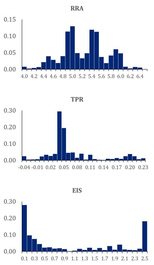
time-variation in the growth rate of wealth within each household group. This identifi-
cation strategy that exploits the time pattern of wealth accumulation is a methodological
contribution of our paper.

   Our main empirical findings are as follows.

    First, our data analysis uncovers considerable heterogeneity in wealth accumulation and
portfolio composition across the Swedish population. Average wealth-income ratios vary
intuitively with the riskiness of income and the level of education: among groups with the
lowest income risk and lowest education, the average wealth-income ratio is 3.6, whereas it
is 6.0 among groups with the highest income risk and highest level of education. There is
also considerable heterogeneity unrelated to these variables: within each category of income
risk and education, the standard deviation of the wealth-income ratio exceeds 3.0 across
the groups we consider. Average risky shares vary little with income risk or education,
averaging between 0.65 and 0.69 across all income risk and education categories, but within
each category the standard deviation of the risky share across groups is substantial, ranging
from 0.19 to 0.25.

   Second, we document time-series and cross-sectional patterns in wealth and portfolio
composition that are broadly consistent with life-cycle financial theory. As households age,
they tend to accumulate wealth and reduce their risky portfolio share. The risky portfolio
share also declines with the wealth-income ratio after controlling for age. Both patterns are
predicted by a life-cycle model in which human capital is safer than risky financial capital.

    Third, we estimate that the average level of risk aversion across Swedish households is
5.24, close to the median level of 5.30. The cross-sectional standard deviation of risk aversion
is 0.47. The ratio of standard deviation to mean is smaller for risk aversion than for the risky
portfolio share because households have human capital in our model; if there were no human
capital, the usual formula for risky portfolio choice under homogeneous beliefs implies that
risk aversion and the risky share must be proportional to one another and therefore must
have the same ratio of standard deviation to mean.

    Fourth, we estimate the average rate of time preference to be 6.18%, well above the
median value of 4.08% because the distribution of time preference rates is right-skewed and
dispersed, with a standard deviation of 6.03%. We estimate negative rates of time preference
for 6.5% of Swedish households; these low values of time preference may in part reflect the
existence of bequest motives that are omitted from our life-cycle model.

    Fifth, we estimate the average EIS to be very close to one at 0.99. The median EIS
however is well below one at 0.42, reflecting a right-skewed distribution with some households
estimated to have EIS above two. The cross-sectional standard deviation of the EIS is

                                               3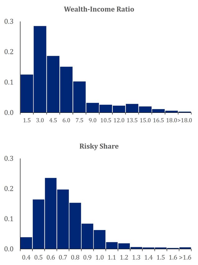
substantial at 0.96. There is a debate in the asset pricing literature about whether the EIS
is less than one, as estimated by Hall (1988), Yogo (2004) and others in time-series data, or
greater than one, as assumed by Bansal and Yaron (2004) and a subsequent literature on
long-run risk models. We find that the EIS is less than one for 60% of households, and even
less than the reciprocal of risk aversion for 35% of households, while it is greater than one
for 40% of households. This much cross-sectional variation suggests that aggregate results
are likely to be sensitive to the way in which households are aggregated and are unlikely to
be precise, consistent with large standard errors reported by Calvet and Czellar (2015) in a
structural estimation exercise using aggregate data.

    Sixth, our estimates of preference parameters are weakly cross-sectionally correlated.
The correlation between risk aversion and the EIS is weakly positive at 0.11, in contrast
with the perfect negative correlation between log risk aversion and the log EIS that we
would find if all households had power utility with heterogeneous coefficients. The rate
of time preference is negatively correlated with both risk aversion (−0.28) and the EIS
(−0.29), implying a tendency for patient people to be both cautious and willing to substitute
intertemporally. The weak correlations across preference parameters imply that Swedish
household behavior is heterogeneous in multiple dimensions, not just one. A single source of
heterogeneity omitted from our model, such as heterogeneity in household beliefs about the
equity premium, would not generate this multidimensional heterogeneity in our preference
estimates.

     Seventh, there are some interesting correlations between our parameter estimates, the
moments we use for estimation, and exogenous charateristics of households. Risk aversion
is lower for households working in risky sectors: households in these sectors invest somewhat
more conservatively, but not as conservatively as they would do if they understood their
income risk and had the same risk aversion as households working in safer sectors. Risk
aversion is also lower for households with higher education: these households tend to have
higher wealth-income ratios, but similar risky shares. Both these patterns are consistent
with the hypothesis that risk-tolerant households choose to acquire education and select risky
occupations, but they could also result from households’ failure to understand the portfolio
choice implications of their income risk exposure and wealth accumulation.

    The rate of time preference is negatively correlated (−0.30) with the initial wealth-income
ratio of each household group, and positively correlated (0.35) with the average growth rate
of the wealth-income ratio. These patterns reflect the fact that households who enter our
sample with a low wealth-income ratio accumulate wealth more rapidly, but not as much
more rapidly as they would do if they were as patient as households with a higher initial
wealth-income ratio. In other words, the symptom of a high rate of time preference in our
data is a tendency to accumulate retirement savings later in life, catching up belatedly with

                                              4
those who saved earlier in life.
Our paper is related to a large literature on household portfolio choice over the life cy-
cle, including Campbell and Viceira (2002), Ameriks and Zeldes (2004), Cocco, Gomes, and
Maenhout (2005), and Fagereng, Gottlieb, and Guiso (2017). Guiso and Sodini (2013) pro-
vide a comprehensive survey. Several recent papers have highlighted the role of target date
funds as a low-cost way to implement a declining age profile in the risky portfolio share,
but have also explained ways in which these funds fall short of the theoretical optimum
(Dahlquist, Setty, and Vestman 2018, Parker, Schoar, and Sun 2020). Our use of compre-
hensive administrative data from Sweden follows a series of papers by Calvet, Campbell,
and Sodini (2007, 2009a, 2009b), Calvet and Sodini (2014), Betermier, Calvet, and Sodini
(2017), and Bach, Calvet, and Sodini (2020).
A smaller literature on heterogeneity in portfolio choice has recently tried to relate ob-
served household behavior to underlying heterogeneity in preferences and beliefs (Meeuwis
et al 2018, Giglio et al 2019). Relative to this literature, we observe more households over a
longer period of time and have more complete data on wealth and portfolio allocation, but
we lack data on potentially heterogeneous beliefs.
The organization of the paper is as follows. Section 2 explains how we measure house-
hold wealth and its allocation to safe and risky assets, describes the creation of household
groups, and reports summary statistics for the wealth-income ratio and the risky share across
these groups. Section 3 presents the life-cycle model and household labor income processes.
Section 4 discusses preference parameter identification and develops our estimation method-
ology. Section 5 reports empirical results on the cross-section of household preferences, and
section 6 concludes. An online appendix provides additional details about our empirical
analysis and estimation technique.
2 Measuring Household Wealth and Asset Allocation
Our empirical analysis is based on the Swedish Wealth and Income Registry, a high-quality
administrative panel that has been used in earlier research. The registry provides the income,
wealth, and debt of every Swedish resident. Income data are available at the individual level
from 1983 and can be aggregated to the household level from 1991. Wealth data are
available from 1999. The wealth data include bank account balances, holdings of financial
assets, and real estate properties measured at the level of each security or property. The
registry does not report durable goods, private businesses, or defined-contribution (DC)
retirement wealth, but we augment the dataset by imputing DC contributions using income
5data and the administrative rules governing DC pensions in Sweden. We accumulate these
contributions to estimate DC wealth at each point in time, and use a similar procedure to
calculate entitlements to DB pension income. All our data series end in 2007.
2.1 The Household Balance Sheet
We first aggregate the data to the household level. We define a household as a family living
together with the same adults over time. The household head is the adult with the highest
average non-financial disposable income; or, if the average income is the same, the oldest;
or, if the other criteria fail, the man in the household.
We measure four components of the household balance sheet: liquid financial wealth, real
estate wealth, DC retirement savings, and debt. We define the total net wealth of household
h at time t, Wh,t , as
Wh,t = LWh,t + REh,t + DCh,t − Dh,t , (1)
where LWh,t is liquid financial wealth, REh,t is real estate wealth, DCh,t is DC retirement
wealth, and Dh,t is debt. In aggregate Swedish data in 1999, the shares of these four
components in total net wealth are 36%, 76%, 13%, and −25%, respectively.
Liquid financial wealth is the value of the household’s bank account balances and holdings
of Swedish money market funds, mutual funds, stocks, capital insurance products, derivatives
and directly held fixed income securities. Mutual funds include balanced funds and bond
funds, as well as equity funds. We subdivide liquid financial wealth into cash, defined as the
sum of bank balances and money market funds, and risky assets.
Real estate consists of primary and secondary residences, rental, commercial and in-
dustrial properties, agricultural properties and forestry. The Wealth and Income Registry
provides the holdings at the level of each asset. The pricing of real estate properties is based
on market transactions and tax values adjusted by a multiplier, as in Bach, Calvet, and
Sodini (2020).
Debt is the sum of all liabilities of the household, including mortgages and other per-
sonal liabilities held outside private businesses.1 Since Swedish household debt is normally
1
Because we do not observe durable goods (such as appliances, cars and boats), the value of household
debt can exceed the value of the assets we oberve for some households. To avoid this problem, the debt
variable Dh,t is defined as the minimum of the total debt and real estate wealth reported in the registry.
This approach is consistent with the fact that we proxy the borrowing rate by the average mortgage rate
offered by Swedish institutions.
6floating-rate, we treat debt as equivalent to a negative cash position but paying a borrowing
rate that is higher than the safe lending rate.
The hardest balance sheet component to measure is DC retirement wealth. We do not
measure this directly but impute it by reconstructing the details of the Swedish pension
system, as we discuss in the next subsection. This detailed pension analysis also enables
us to measure each household’s entitlement to defined benefit (DB) pension payments in
retirement.
As described here, the household balance sheet excludes durable goods and private busi-
nesses, whose values are particularly difficult to measure. Private businesses are an impor-
tant component of wealth for the wealthiest households in Sweden (Bach, Calvet, and Sodini
2020), but unimportant for most Swedish households.
2.2 Pension Imputation
The Swedish pension system consists of three pillars: occupational pensions, state pensions,
and private pensions. We discuss these in turn. Full details are provided in an online
appendix.
Occupational pensions were introduced to Sweden in 1991. They are regulated for the
vast majority of Swedish residents by four collective agreements that cover different occu-
pational categories: blue-collar private-sector workers, white-collar private-sector workers,
central government employees, and local government employees. These agreements specify
workers’ monthly pension contributions, the fraction directed to defined benefit (DB) and
defined contribution (DC) pension plans, and the DC choices available to workers.
The collective agreements specify DC contributions as a percentage of pension qualifying
income. These contributions are invested through insurance companies in either variable
annuity products (called TradLiv in Sweden), or in portfolios of mutual funds, chosen by
workers from a selection provided by the insurance company. There are also DB contribu-
tions which have been declining over time relative to DC contributions under the terms of
the agreements, in a gradual transition from a DB to a DC pension system. We are able
to impute both DC contributions and DB entitlements at the household level by following
the rules of the collective agreements as detailed in the appendix. We can do this accurately
because the data on pension qualifying income is available from 1991 (the year occupational
pensions were introduced) and because the DB collective pension payouts are a function of
at most the last 7 years of pension qualifying income during working life.
7The state pension system requires each worker in Sweden to contribute 18.5% of their
pension qualifying income: 16% to the pay-as-you-go DB system and the remaining 2.5%
to a DC system (called premiepension system or PPM). DC contributions are invested in
a default fund, that mirrors the world index during our sample period, unless the worker
opts out and chooses a portfolio of at most 5 funds among those offered on the state DC
platform (on average around 650 funds from 1999 to 2007). State DB payouts are a function
of the pension qualifying income earned during the entire working life. Since our individual
income data begin in 1983, we cannot observe the full income history for older individuals
in our dataset. To handle this, we back-cast their income back to the age of 25 by using
real per-capita GDP growth and inflation before 1983, as explained in the appendix. We
then use the state DB payout rules to impute state DB pension payments for each individual
retiring during our sample period.
Defined contribution private pensions have existed in Sweden for a long time but our
dataset provides us with individual private pension contributions from 1991.2 We assume
that these contributions are invested in the same way as occupational and state DC contri-
butions. We follow Bach, Calvet and Sodini (2020) and allocate 58% of the aggregate stock
of private pension wealth in 1991 to workers.3 Across workers, we allocate pension wealth
proportionately to their private pension contributions in 1991.
To calculate DC retirement wealth at each point in time, we accumulate contributions
from all three pillars of the Swedish pension system. To do this we assume that occupational
and private DC equity contributions are invested in the MSCI equity world index, without
currency hedging, earning the index return less a 70 basis point fee which prevailed during
our sample period. This assumption reflects the high degree of international diversification
observed in Swedish equity investments (Calvet, Campbell, and Sodini 2007). In the state
DC system, we follow the investment policy and cost of the system’s default fund and assume
that equity contributions are invested in the unhedged MSCI equity world index but pay a
fee of only 15 basis points. The equity share in each household’s occupational and private
DC retirement portfolio is rebalanced with age following the representative age pattern of
life-cycle funds available in Sweden during our sample period. The equity share in the state
DC system mirrors the allocation rules of the system’s default fund: a 130% levered position
in the world index up to the age of 55, which is then gradually rebalanced with age to an
increasingly conservative portfolio as described in the appendix. We assume that all DC
wealth not invested in equities is invested in cash.
2
Our dataset contains exact information on private pension contributions from 1994, and only reports a
capped version of the variable from 1991. We impute full contributions from 1991 to 1993 taking into account
both age effects and individual savings propensities in subsequent years, as explained in the appendix.
3
This allocation is chosen to satisfy the condition that imputed pension wealth should be roughly the
same just before and just after retirement.
8DC retirement wealth accumulates untaxed but is taxed upon withdrawal. To convert
pre-tax retirement wealth into after-tax units that are comparable to liquid financial wealth,
we assume an average tax rate τ on withdrawals (estimated at 32% which is the average
tax rate on nonfinancial income paid by households with retired heads over 65 years old)
and multiply pre-tax wealth by (1 − τ ). In the remainder of the paper, we always state
retirement wealth in after-tax units.
2.3 Household Asset Allocation
Our objective is to match the rich dataset of household income and asset holdings to the
predictions of a life-cycle model, which will allow us to estimate household preferences. To
accomplish this, we need to map the complex data into a structure that can be related to a
life-cycle model with one riskless and one risky asset. We do this in three stages. First we map
all individual assets to equivalent holdings of diversified stocks, real estate, or cash. Second,
we assume a variance-covariance matrix for the excess returns on stocks and real estate over
cash that enables us to compute the volatility of each household portfolio. Third, we assume
that all household portfolios earn the same Sharpe ratio so that the volatility of the portfolio
determines the expected return on the portfolio. Equivalently, we convert the volatility
into a “risky share” held in a single composite risky asset. For ease of interpretation, we
normalize that risky asset to have the same volatility as a world equity index.
At the first stage, we treat liquid holdings of individual stocks, equity mutual funds,
and hedge funds as diversified holdings of the MSCI world equity index.4 We treat liquid
holdings of balanced funds and bond funds as portfolios of cash and stocks, with the share in
stocks given by the beta of each fund with the world index.5 We assume that unclassifiable
positions in capital insurance, derivatives, and fixed income securities are invested in the
same mix of cash and stocks as the rest of liquid financial wealth. We treat all real estate
holdings as positions in a diversified index of Swedish residential real estate, the FASTPI
index. We assume that DC retirement wealth is invested in cash and the MSCI equity world
index as described in section 2.2.
This mapping gives us implied portfolio weights in liquid stocks, real estate, and DC
stocks in the net wealth of each household. For household h at time t, write these weights
4
This reflects the global diversification of Swedish equity portfolios documented by Calvet, Campbell,
and Sodini (2007). It abstracts from underdiversification, which the same paper shows is modest for most
Swedish households although important for a few. The impact of underdiversification in liquid wealth is
further reduced when one takes account of DC retirement wealth as we do in this paper.
5
We cap the estimated fund beta at 1, and use the cross-sectional average fund beta for funds with less
than 24 monthly observations.
9h h h e e e
as ωS,t , ωRE,t , and ωDC,t , and the corresponding excess returns as RS,t+1 , RRE,t+1 , RDC,t+1 .
The excess return on household net wealth is then given by:
e h e h e h e h h h e
Rt+1 = ωS,t RS,t+1 + ωRE,t RRE,t+1 + ωDC,t RDC,t+1 + (1 − ωS,t − ωRE,t − ωDC,t )RD,t+1 , (2)
e
where RD,t+1 is the borrowing rate in excess of the Swedish t-bill. The second stage of our
analysis is to calculate the variance of the excess return on household net wealth. Since the
borrowing rate is deterministic, we only need to consider the vector ωth = (ωS,t
h h
, ωRE,t h
, ωDC,t )0 ,
e
and we can calculate the variance of Rt+1 as
0
σ 2 (Rh,t+1
e
) = ωh,t Σ ωh,t , (3)
where Σ is the variance-covariance matrix of e
(RS,t+1 e
, RRE,t+1 e
, RDC,t+1 )0 .
To estimate the elements of Σ, we assume that cash earns the Swedish one-month risk-free
rate net of taxes, that liquid equity earns the MSCI world index return less a 30% long-term
capital income tax rate (Du Rietz et al. 2015), that real estate earns the FASTPI index
return less a 22% real estate capital gain tax rate, and that stocks held in DC plans earn the
pre-tax MSCI world index return before the adjustment of their value to an after-tax basis.
Using data from 1984–2007, we estimate the post-tax excess return volatility for stocks at
13.3% and for real estate at 5.5%, with a correlation of 0.27. The pre-tax excess stock return
volatility is 19%.
In the third stage of our analysis, we define a numeraire asset, the aggregate Swedish
portfolio of cash, stocks, and real estate scaled to have the same volatility as the after-tax
global equity index return:
e 0 e
RN,t+1 = (1 + L)(ωagg,t Rt+1 ). (4)
e
Here RN,t+1 is the return on the numeraire asset and ωagg,t is the vector containing the
weights of equity, real estate and the DC retirement portfolio in the aggregate net wealth of
all Swedish households in our sample. The scaling factor L is chosen so that the volatility of
e
RN,t+1 is equal to the volatility of the after-tax return in local currency on the global equity
index.
The empirical risky share αh,t is the ratio of the volatility of household h’s portfolio to
the volatility of the numeraire asset:
e e
αh,t = σ Rh,t+1 /σ RN,t+1 , (5)
where household portfolio volatility is computed from equation (3). This approach implicitly
assumes that all households earn the same Sharpe ratio on their risky assets, but guarantees
that the standard deviation of a household’s wealth return used in our simulations coincides
with its empirical value. A value of one for αh,t says that a household’s portfolio has the
same volatility, 13.3%, as if it invested solely in stocks held outside a retirement account,
without borrowing or holding cash.
102.4 Composite Households
The full Swedish Income Registry data set contains almost 41 million household-year ob-
servations over the period 1999 to 2007, but we impose several filters on the panel. We
exclude households in which the head is a student, working in the agricultural sector, retired
before the start of our sample, missing information on education or sector of employment,
or outside the set of cohorts we consider. We also exclude households that do not have
observations in all years between 1999 and 2007 and households that do not participate in
risky asset markets outside retirement accounts. Finally, to limit the impact of the wealth-
iest households (for whom our measurement procedures may be less adequate), we exclude
households whose financial wealth is above the 99th percentile of the wealth distribution in
1999. After imposing these filters we have a balanced panel with about 363,000 households
and 3.3 million household-year observations.
We classify households by three levels of educational attainment: (i) basic or missing
education, (ii) high school education, and (iii) post-high school education. We also classify
households by 12 sectors of employment. Within each education level, we rank the sectors by
their total income volatility and divide them in three categories. In this way we create a 3×3
grid of 9 large education/sector categories where the sectors of employment are aggregated
by income volatility.6
We subdivide each of these categories using a two-way sort by deciles of the initial wealth-
income ratio and the initial risky share. We use the lowest two and highest two deciles and
the middle three quintiles, giving us a 7 × 7 grid of 49 bins for the initial wealth-income ratio
and the risky share.7 We further subdivide by 13 cohorts (birth years from 1947 to 1959) to
create 5733 = 9 × 49 × 13 groups. After excluding some small groups that do not contain
members in each year from 1999 to 2007, our final sample is a perfectly balanced panel of
4151 groups.
The median group size across years is 63 households, but the average group size is larger
at about 86 households. The difference reflects a right-skewed distribution of group size,
with many small groups and a few much larger ones. The group-level statistics we report in
the paper are all size-weighted in order to reflect the underlying distributions of data and
preference parameters at the household level.
6
The estimation of income volatility is described in section 3, and details of the sectoral income risk
classification are provided in table IA.2 in the online appendix.
7
The wealth-income and risky share breakpoints are set separately in each of the 9 categories. This
ensures that across categories we have the same proportion of households at each of the 7 risky share and
wealth-income levels. However, the number of households can differ across the 49 bins defined by the two-way
sort, to the extent that the wealth-income ratio and the risky share are cross-sectionally correlated.
11We treat each group as a composite household, adding up all wealth and income of
households within the group. Because we assume scale-independent Epstein-Zin preferences,
we scale wealth by income and work with the wealth-income ratio as well as the implied risky
share held in our composite numeraire asset.
2.5 Cross-Section of the Risky Share and wealth-income Ratio
We now consider the cross-section of the wealth-income ratio and risky share, averaging
across all years in our sample.
The top panel of Table 1 shows the variation in average wealth-income ratios and risky
portfolio shares across groups with each level of education and sectors of employment with
each level of income risk, averaging across cohorts and the subdivisions by initial wealth-
income ratio and risky share. For the purpose of computing these summary statistics, house-
holds in each group are treated as a single composite household that owns all wealth and
receives all income of the group, and groups are weighted by the number of households they
contain. Average wealth-income ratios vary widely from 3.6 to 6.0, while average risky
shares vary in a narrow range from 65% to 69%. Within each sector, average wealth-income
ratios are higher for more educated households, particularly those with post-high school ed-
ucation, but average risky portfolio shares vary little with education. Across sectors, the
level of income risk has a a strong positive effect on the wealth-income ratio and a weak
negative effect on the risky portfolio share.
The category averages in the top panel of Table 1 conceal a great deal of dispersion
across disaggregated groups of households. This is shown by the bottom panel of Table
1, which reports the standard deviations of the wealth-income ratio and the risky portfolio
share across groups in each of the nine categories of education and sectoral income risk.
The standard deviations of the risky share are consistently in the range 19–25%, while the
standard deviations of the wealth-income ratio are in the range 3.0–3.9. Across all 4151
groups, the average wealth-income ratio has a mean of 4.7 with a standard deviation of 3.6,
while the average risky share has a mean of 67% with a standard deviation of 22%.8
Figure 1 plots the cross-sectional distributions of the time-series average wealth-income
ratio and risky share across all groups, size-weighting the groups to recover the underlying
8
The aggregation of households into groups naturally reduces the dispersion that is visible in the
household-level data. Across all individual households in our dataset the average wealth-income ratio
is 6.5 with a standard deviation of 185. After winsorizing the underlying household distribution at the 99th
percentile, the average falls to 4.6 and the standard deviation falls to 4.0. The average risky share across
all individual households is 71% with a standard deviation of 43%.
12household distribution. The wealth-income ratios have a strongly right-skewed distribution,
with many households having only a year or two of income accumulated, and a few having
well over a decade of income. The risky shares also have a right-skewed cross-sectional
distribution including some probability mass above 1 (corresponding to a portfolio volatility
above 13.3%).
The cross-sectional variation in wealth and asset allocation documented in Table 1 and
Figure 1 suggests that it will be difficult to account for Swedish household behavior without
allowing for cross-sectional variation in preferences. However, we have not yet accounted
for cross-sectional variation in the wealth-income ratio at the start of our sample, which may
reflect past shocks to income and wealth as well as heterogeneous savings behavior driven
by preferences. We now develop a life-cycle model that we can use to estimate preferences
from the evolution of wealth and asset allocation during our sample period, taking as given
the initial wealth-income ratio and the income and financial returns received in each year of
our sample.
3 Income Process and Life-Cycle Model
In this section, we present the labor income process and the life-cycle model of saving and
portfolio choice that are used to estimate household preferences.
3.1 Labor Income Process
We consider the labor income specification of Cocco, Gomes, and Maenhout (2005):
log(Yh,t ) = ac + b0 xh,t + νh,t + εh,t , (6)
where Yh,t denotes real income for household h in year t, ac is a cohort fixed effect, xh,t is
a vector of characteristics, νh,t is a permanent random component of income, and εh,t is a
transitory component.
We enrich the Cocco, Gomes, and Maenhout model by distinguishing between shocks
that are common to all households in a group and shocks that are specific to each household
in the group. To simplify notation, we neglect the group index g in the rest of this section.
We assume that the permanent component of income, νh,t , is the sum of a group-level
component, ξt , and an idiosyncratic component, zh,t :
νh,t = ξt + zh,t . (7)
13The components ξt and zh,t follow independent random walks:
ξt = ξt−1 + ut , (8)
zh,t = zh,t−1 + wh,t . (9)
The transitory component of income, εh,t , is by contrast purely idiosyncratic. This
fits the fact that group average income growth in our Swedish data is slightly positively
autocorrelated, whereas it would be negatively autocorrelated if transitory income had a
group-level component.
Finally, we assume that the three income shocks are i.i.d. Gaussian:
(ut , wh,t , εh,t )0 ∼ N (0, Ω) (10)
where Ω is the diagonal matrix with diagonal elements σu2 , σw2 , and σe2 .
We estimate the income process from consecutive observations of household yearly income
data over the period 1992 to 2007, excluding the first and last year of labor income to avoid
measuring annual income earned over less than 12 months. In each year, we winsorize
non-financial real disposable income to 1000 kronor or about $150.9 . We consider the
total income received by all members of the household, but classify households by the head’s
education level and age. Since the vast majority of Swedish residents retire at 65, we consider
two age groups: (i) non-retired households less than 65 and older than 19, and (ii) retired
households that are at least 65.
For active households younger than 65, we estimate b by running pooled regressions of
equation (6) for each of the three education groups. As in Cocco, Gomes, and Maenhout
(2005), the vector of explanatory variables xh,t includes age dummies. We then regress the
estimated coefficients of age dummies on a third-degree polynomial in age and use the fitted
third-degree polynomial in our life-cycle model.
To estimate income risk, we further divide households of the same education group into
business sector categories. σu is estimated by averaging the regression residuals within each
education-business sector group, and by computing the sample standard deviation of the
resulting income innovations. We then apply the Carroll and Samwick (1997) decomposition
to the regression residuals demeaned at group level to estimate the permanent and transitory
idiosyncratic income risks, σw2 , and σe2 , of each education-business sector group.
We proceed in two steps. First, we implement the procedure above on 36 education - busi-
ness sector groups obtained by dividing households of each of the three eduction groups into
9
We also winsorize the pooled data from above at 0.01% level to take care of extreme outliers at the top
of the income distribution
14the 12 business sectors corresponding to the first digit of the SNI industry code. Equipped
with income risk estimates for each of the 36 groups, we aggregate business sectors into three
categories of total income risk for each education level. 10 Second, we re-apply the procedure
above to estimate income risk for the resulting nine education - business groups.
For retired households, we impute the state and occupational after-tax pension benefit of
each individual from 1999 to 2007, as explained in the online appendix. We fill forward the
imputed pension benefit in real terms until 2007 at individual level, and aggregate income
at the household level in each year. The replacement ratio is estimated for each education
group as the fraction of the average income of non-retired 64-year-old households to the
average income of retired 65-year-old households across the 1999 to 2007 period.
Figure 2 illustrates the estimated age-income profiles for our three education groups.
The profiles are steeper than profiles estimated in the US.11
3.2 Income Risks Across Groups
Table 2 reports the estimated standard deviations of group-level income shocks (permanent
by assumption) and of permanent and transitory idiosyncratic income shocks, across the
nine categories defined by three levels of education and sectors of employment sorted into
three categories by their total income risk.
Looking across sectors, group-level income volatilities and permanent idiosyncratic in-
come volatilities vary relatively little, but transitory idiosyncratic income volatilities are
considerably higher for high-risk sectors. The online appendix reports the underlying sec-
tors that fall in each category. The patterns are intuitive, with relatively little transitory
income risk in the public sector and in mining and quarrying, electricity, gas, and water
supply, and relatively high transitory income risk in hotels and restaurants, real estate ac-
tivities, construction for less educated workers, and the financial sector for more educated
workers.
Table 2 also shows that educated households, particularly those with higher education,
face higher transitory income risk and lower permanent income risk than less educated house-
holds. This pattern is consistent with Low, Meghir, and Pistaferri (2010), but it contrasts
10
We obtain very similar rankings by sorting with idiosyncratic transitory income risk.
11
Dahlquist, Setty, and Vestman (2018) estimate income profiles for Sweden with a pronounced hump
shape and lower income towards the end of working life. They use a model that excludes cohort effects,
thereby estimating the age-income profile in part by comparing the incomes of households of different ages
at a point in time. This procedure is biased if different cohorts receive different lifetime income on average.
We obtain similar estimates when we exclude cohort effects from our model of income.
15with earlier studies showing the opposite pattern in the United States. The explanation
is likely due to the fact that in Sweden, uneducated workers face lower unemployment risk
and enjoy higher replacement ratios than in many other countries, while educated workers
face relatively high income losses when they do become unemployed. This results from the
following features of the Swedish labor market. First, it is straightforward for companies
to downsize divisions, but extremely difficult for them to lay off single individuals unless
they have a high managerial position. Second, companies that need to downsize typically
restructure their organizations by bargaining with unions. Third, unions are nationwide or-
ganizations that span large areas of employment and pay generous unemployment benefits.
Fourth, the pay cut due to unemployment is larger for better paid jobs. After an initial
grace period, an unemployed person will be required to enter a retraining program or will
be assigned a low-paying job by a state agency. All these features imply that unemployment
is slightly more likely and entails a more severe proportional income loss for workers with
higher levels of education.12
We have already noted in discussing Table 1 that average wealth-income ratios tend to
be higher in sectors with riskier income. This pattern is intuitive given that labor income
risk encourages precautionary saving. However, there is little tendency for risky portfolio
shares to be lower in sectors with riskier income. Table 3 further explores these effects by
regressing the average wealth-income ratio and risky share on age, total income volatility,
and dummies for high school and post-high school education. All regressions also include
year fixed effects.13
The first column of the table shows that the average wealth-income ratio increases with
age and with income volatility. This is consistent with the view that wealth is accumulated
in part to finance retirement, and in part as a buffer stock against temporary shocks to
income. In addition, the average wealth-income ratio increases with the level of education.
The second column shows that the average risky share decreases with age, but income
risk and education are not significant predictors of the average risky share although the
coefficient on income risk is negative as one might expect. The third column adds the
average wealth-income ratio as a predictor for the risky share, and finds a negative effect.
After controlling for the wealth-income ratio, income risk has a significantly positive effect
on the risky share. This finding suggests that households with risky income tend to have
lower risk aversion, and indeed our life-cycle model allows us to document such a pattern.
12
See Brown, Fang, and Gomes (2012) for related research on the relation between education and income
risk.
13
We do not include cohort effects in this table. It is well known that unrestricted time, age, and cohort
effects cannot be identified (Ameriks and Zeldes 2004, Fagereng, Gottlieb, and Guiso 2017). Here we use
unrestricted time effects, a linear age effect, and exclude cohort effects. We exclude time effects and allow
cohort effects in our analysis of preferences, as we discuss below.
16The negative effects of age and the wealth-income ratio on the risky share are consistent
with the predictions of a simple static model in which labor income is safe and tradable,
so that human capital is an implicit cash holding that tilts the composition of the financial
portfolio towards risky assets (Bodie, Merton, and Samuelson 1992, Campbell and Viceira
2002 p.163, Campbell 2018 p.309). Older households have fewer earning years remaining so
their human capital is lower; and at any given age, households with a higher wealth-income
ratio have more financial capital relative to human capital. In both cases the tilt towards
risky assets is reduced.
We work with a richer lifecycle model in which labor income is risky and nontradable,
but that model implies a similar pattern of age and wealth effects on the risky share. We
will use our model to study the distribution of preferences across households with higher or
lower education working in riskier or safer sectors.
3.3 Life-Cycle Model
We consider a standard life-cycle model, very similar to the one in Cocco, Gomes and
Maenhout (2005).
Households have finite lives and Epstein-Zin utility over a single consumption good. The
utility function Vt is specified by the coefficient of relative risk aversion (RRA) γ, the time
discount factor δ or equivalently the time preference rate (TPR) − log(δ), and the elasticity
of intertemporal substitution (EIS) ψ. Vt satisfies the recursion
h i 1
1−1/ψ 1−γ (1−1/ψ)/(1−γ) 1−1/ψ
Vt = Ct + δ Et pt,t+1 Vt+1 , (11)
where pt,t+1 denotes the probability that a household is alive at age t+1 conditional on being
alive at age t. Utility, consumption, and the preference parameters γ, δ, and ψ all vary across
households but we suppress the household index h in equation (11) for notational simplicity.
The age-specific probability of survival, pt,t+1 , is obtained from Sweden’s life table.
Capturing the wealth accumulation of young households poses several problems for life-
cycle models which do not include housing purchases, transfers from relatives, investments
in education, or changes in family size. In addition it is well-known that such models predict
an extremely high equity share at early ages which is hard to reconcile with our data. For
this reason, we focus on the stage of the life-cycle during which households have substantial
retirement saving and initialize our model at age 40. We follow the standard notational
convention in life-cycle models and let the time index in the model, t, start at 1, so that t is
calendar age minus 39. Each period corresponds to one year and agents live for a maximum
of T = 61 periods (corresponding to age 100).
17Matching the behavior of retirees is also hard for simple life-cycle models that do not
incorporate health shocks or bequest motives. For this reason, we only consider the model’s
implications for ages 40 to 60 years. Our model includes no bequest motive, because it
would be difficult to separately identify the discount factor and the bequest motive using
our sample of households in the 40 to 60 age group, and we prefer not to add one more
weakly identified parameter. Our estimates of the time preference rate can be viewed as
having a downward bias due to the absence of a bequest motive in the model.
Before retirement households supply labor inelastically. The stochastic process of the
household labor income, Yh,t , is described in Section 3.1. All households retire at age 65, as
was typically the case in Sweden during our sample period, and we set retirement earnings
equal to a constant replacement ratio of the last working-life permanent income.
Consistent with the discussion in Section 2, total wealth, Wh,t , consists of all the assets
held by the household. For tractability, we assume in the model that total wealth is invested
every period in a one-period riskless asset (bond) and a composite risky asset. In each period
we recalibrate beginning-of-period wealth to the level observed in the data and use the model
to predict end-of-period wealth.
The household chooses its consumption level Ch,t and risky portfolio share αh,t every
period, subject to a constraint that financial wealth is positive—that is, the household cannot
borrow against future labor income to finance consumption. We do allow borrowing to
finance a risky asset position, that is, we allow αh,t ≥ 1. Household wealth satisfies the
budget constraint
e
Wh,t+1 = (Rf + αh,t Rt+1 )(Wh,t + Yh,t − Ch,t ), (12)
e
where Rt+1 is the return on the composite numeraire asset in excess of the risk-free rate Rf .
e
The excess return Rt+1 is Gaussian N (µr , σr2 ).
3.4 Calibrated Parameters
The parameters of our life-cycle model can be divided into those describing the income
process, and those describing the properties of asset returns. For income, we have age profiles
and retirement replacement ratios as illustrated in Figure 2, and the standard deviations of
permanent group-level, permanent idiosyncratic, and transitory idiosyncratic income shocks
reported in Table 2.
In our model we assume that all safe borrowing and lending takes place at a single safe
interest rate of 2.0%. This is calibrated as a weighted average of a safe lending rate of
0.8% and the average household borrowing rate of 3.6%, using the cross-sectional average
18household debt level to construct the average.14
We set the volatility of the numeraire risky asset at 13.3%, which is equal to the volatility
of post-tax excess stock returns as discussed in section 2.3. We assume that the average
excess return on the numeraire asset over the 2.0% safe interest rate is 3.5%, the same as
the average post-tax equity premium on the MSCI world index in local currency over the
period 1984–2007. Putting these assumptions together, we assume a Sharpe ratio of 0.26.
For robustness, in the online appendix we re-estimate our model using a higher Sharpe ratio
of 0.5.
The remaining parameter that must be calibrated is the correlation between the nu-
meraire risky asset return and group-level income shocks. We estimate this correlation
lagging the risky asset return one year, following Campbell, Cocco, Gomes, and Maenhout
(2001), to capture a delayed response of income to macroeconomic shocks that move asset
prices immediately. Empirically the correlation is very similar across the 9 education-sector
categories, and we set it equal to the average value of 0.44. This is intermediate between a
lower value of 0.27 for the correlation estimated using only stock returns, and a higher value
of 0.87 for the correlation estimated using only real estate returns.
The correlation between the numeraire risky asset return and individual income growth
is much smaller than 0.44, because most individual income risk is idiosyncratic. To il-
lustrate with a representative example, a household with group-level standard deviation of
3%, permanent idiosyncratic standard deviation of 8%, and transitory idiosyncratic stan-
dard deviation of 12% would have a correlation with the numeraire risky asset of 0.20 for
its permanent income shocks and only 0.11 for its total income shocks. Nonetheless, the
group-level income correlation plays an important role in our model, because it helps to
choke off household demand for risky assets even at moderate levels of risk aversion.
4 Identification and Estimation
This section explains our procedure for estimating household preference parameters. Using
the calibrated income and asset-return parameters as inputs, we solve the life-cycle model for
each of our household groups on a multi-dimensional grid for the three unknown preference
parameters, using interpolation methods to allow us to consider parameter combinations that
14
Our model would allow us to assume that households pay a higher rate when they borrow to buy the
numeraire asset (that is, when they have a risky share greater than one). However, this assumption would
not be a better approximation to reality than the one we make, since households who borrow to buy housing
pay the borrowing rate even when their risky share is below one.
19are not on the initial grid. For each combination of parameters we consider, after solving
the model we simulate it conditioning on the observed wealth-income ratio at the beginning
of each period and feeding in historically realized group-level income shocks and shocks
to returns on the composite risky asset. From these simulations we calculate the model’s
implied wealth accumulation and asset allocation, which we then use to construct an indirect
inference estimator of the preference parameters that minimizes a measure of the discrepancy
between the simulated and observed data.
We consider many household groups so that we can indeed measure the cross-sectional
distribution of preferences, but we do not estimate the model for each individual household
for two main reasons. First, by grouping households into bins we hope to eliminate, or at
least significantly decrease, the impact of idiosyncratic events that they might face and which
we do not capture in our model. Second, the use of multiple households allows us to derive
properties for our estimator relying on cross-sectional asymptotics as groups become large.
In the following subsections we explain why parameter identification for Epstein-Zin
preferences is challenging; we motivate our identification strategy using simulations of our
model; and we present our indirect inference estimator and discuss its asymptotic properties.
4.1 The Identification Challenge
Our goal is to identify three separate preference parameters: the coefficient of relative risk
aversion (RRA) γ, the time discount factor δ or equivalently the time preference rate (TPR)
− log(δ), and the elasticity of intertemporal substitution (EIS) ψ. In a model with incomplete
markets all three parameters affect both portfolio shares and wealth accumulation making
their identification non-trivial. The main challenge comes from separately identifying the
time discount factor and the EIS, as we discuss next.
The Euler equation for the return on the optimal portfolio is given by
" − ψ1 ψ1 −γ #
C t+1 Vt+1 P
1 = Et δet+1 Rt+1 (13)
Ct µ(Vt+1 )
P e
where δet+1 = δpt,t+1 , Rt+1 = αRt+1 + (1 − α)Rf , and µ(Vt+1 ) denotes the certainty equivalent
of Vt+1 . This Euler equation holds with equality even though our model has borrowing
constraints, because with labor income risk and a utility function that satisfies u0 (0) = −∞
the agent will always choose to hold some financial assets.15
15
Our model also has short-sales constraints on risky asset holdings, but these do not bind for the middle-
aged households we are considering.
20You can also read